Combining Sliding Mode and Fractional-Order Theory for Maximum Power Point Tracking Enhancement of Variable-Speed Wind Energy Conversion

Abstract

The present study used the wind turbine as a model to focus on combining sliding mode and fractional-order theory for maximum power point tracking (MPPT) enhancement. The combination of sliding mode and fractional-order theory was implemented considering the nonlinearity of the studied model for studying the system’s response. The response of the wind turbine was evaluated after introducing disturbance to the output of the regulator. The results showed the excellent ability of the system to track the reference, regardless of any disturbances. There was no impact of any disturbance on the system or the system’s good follow-up. Moreover, the control scheme showed robustness as regards rejecting the disturbances.

1. Introduction

The world’s growing energy needs stem from a variety of sources such as expanding industries, a rising global population, and other contributing factors. Therefore, alternative energy resources are being searched for by humans, and fossil fuel energy has been considered the major source. Some of the disadvantages of using fossil fuels include the shortage of fossil fuels, the increased cost of power-generating operations, and environmental pollution. This is the reason why renewable energies like wind energy, solar energy, and geothermal energy have been considered. Wind energy has revolutionized the power-generating industry. Wind energy has penetrated the electrical power system, which is continuously increasing.

Wind turbine energy is known among the important systems providing promising outputs for the renewable source of energy. The system works on the principle of capturing the available wind energy to generate mechanical energy through the movement of blades. Further, generators can be used for converting mechanical energy into electrical energy. At times, a direct connection is also developed between the mechanical energy and the windmill of the wind pump. Recently, a new type of wind turbine known as the multi-rotor wind turbine has emerged to address the limitations of traditional turbines. It uses multiple turbines to convert wind energy into mechanical energy to increase the energy harnessed from the wind by up to 30% [1]. Few of the previous studies have provided mathematical models and discussed their advantages and disadvantages compared to conventional turbines [2,3]. The present study has considered the wind turbine system because of the increasing demand for green energy sources and minimizing fossil fuel dependency as the main energy source.

According to REN21, Asia has been considered the largest market for wind turbine energy since the past decade, with 50% added capacity. At the start of 2020, the total capacity of wind turbine energy exceeded 290 GW [4]. The fundamental principle behind wind turbines lies in converting the kinetic energy of wind into electrical power. Manufacturers aim to optimize the extraction of energy from wind resources. Maximum power point tracking (MPPT) efficiently maximizes the conversion of wind energy into electrical power [5]. The peak power points, crucial in determining the energy extracted from wind energy conversion systems (WECSs), directly impact the maximum output of energy. The precision in tracking these peak power points significantly influences the overall efficiency of energy extraction [6].

An essential requirement in wind energy conversion systems is the implementation of a reliable MPPT mechanism, ensuring the extraction of maximum power from wind turbines at an affordable cost. Achieving this necessitates the development of a highly accurate system model, particularly focusing on model-based methodologies. Realizing the maximum potential of WECS involves employing a robust adaptive control system, such as a sliding mode controller (SMC), to optimize power extraction. Modern control strategies, such as sliding mode control and fractional-order control, have shown significant potential in enhancing the performance and robustness of nonlinear systems. Designing the MPPT controller based on the tip speed ratio (TSR) offers a promising approach. Furthermore, integrating a nonlinear controller, like SMC, using fractional-order algorithms enhances stability and response dynamics. The SMC approach, based on the Lyapunov stability theory [7], provides significant benefits compared to traditional methods. It is recognized as one of the most powerful design techniques suitable for a broad spectrum of practical applications, including nonlinear and linear systems.

While fractional-order techniques with PI control can be used to make the control input smooth, it is also important to mention that another possibility to achieve a smooth sliding mode is through the design of higher order sliding mode control (HOSMC) [8]. HOSMC extends the conventional SMC by incorporating higher order derivatives of the sliding variable, which can significantly improve robustness and reduce chattering. Chattering is a common issue in classical SMC, characterized by high-frequency oscillations that can cause wear and tear in mechanical systems. By using HOSMC, these oscillations can be mitigated, leading to a smoother control input and enhanced overall performance of the wind energy conversion system. In this context, the current research aims to investigate aerodynamic systems and various control strategies to achieve the utmost power output. Also, the study aims to focus on a combination of sliding mode and fractional-order theory.

2. Literature Review

WECS stands out as a top contender among renewable energy sources. The variability in the speed and direction of wind energy poses a challenge that directly impacts the extracted power from WECS. The precision in tracking the power peak becomes pivotal in maximizing energy extraction from these systems. In this context, the controller of a WECS assumes a critical role in facilitating MPPT to optimize energy capture.

Scientists and control engineers actively explore various methodologies to optimize power extraction from WECS [9]. The pursuit of MPPT involves categorizing key techniques into four main categories: optimum torque control (OTC), hill climbing search (HCS), power signal feedback (PSF), and TSR. These methods represent diverse approaches aimed at efficiently tracking and harnessing the peak power output of WECS, each employing distinct principles and control mechanisms to enhance energy capture.

The optimum torque control (OTC) concept revolves around the correlation between the rotational speed and torque within a wind turbine generator (WTG). OTC involves computing the rotational speed and deriving the torque as a reference for the controller, establishing a feedback control system [10]. At varying wind speeds, OTC adjusts the generator’s torque to attain its optimal value. This method relies on specific wind turbine parameters (C_pmax and λ_opt), typically provided by the manufacturer [9]. As the wind speed changes, the WTG alters its rotational speed to align the electromagnetic torque accordingly [11]. Researchers and control engineers have implemented diverse controllers based on OTC, including SMC [12,13], fault tolerant control [14], proportional controller [15], zero direct-axis current (ZDC) [16,17], and adaptive dynamic programming (ADP) [18]. These controllers aim to optimize the OTC methodology by employing various control strategies tailored to enhance the efficiency and performance of wind turbine systems.

The OTC method in wind energy systems offers advantages and limitations. It operates independently of real-time wind speed data, contributing to a relatively stable output power from the WTG. However, its applicability is limited, primarily suitable for small to medium-sized turbines and lacking efficacy in larger scale wind turbine systems [10]. In larger WTGs, the rotational speed adjustments are sluggish, leading to decreased efficiency and longer response times. To enhance the MPPT capabilities and increase the annual energy output, integrating a proportional controller with the traditional optimal torque controller is proposed as a potential solution. This integration aims to optimize the system’s performance by augmenting control strategies and maximizing energy extraction.

Researchers and control engineers have implemented various controllers based on the HCS methodology, aiming to optimize the performance of wind turbine systems. These controllers include SMC [9,19], neural network (NN) [10], and fuzzy logic control (FLC) [10,20], among others. In this method, if the operating point lies to the right of the peak point, the controller adjusts it leftward to approach the maximum power point (MPP), and conversely, if the operating point is on the opposite side, it adjusts it rightward. The HCS approach offers several advantages: it does not necessitate precise wind turbine parameters or wind speed data, operates without modes or sensors [21], relies on predefined speed step perturbations to adapt rotor speed to wind speed variations, and requires minimal information from the WT system, making it a relatively efficient and adaptable control strategy in wind energy systems.

The PSF method operates on the premise of an optimal power curve, aiming to extract the maximum power corresponding to the prevailing wind speed within this curve [22,23]. This approach utilizes a control system designed to achieve MPPT by adjusting the rotational speed of the wind turbine, guided by the feedback obtained from the power signal. An alternative method within PSF involves determining the optimal rotational speed for different wind speeds, essentially establishing a reference power trajectory based on power and rotational speed. This methodology hinges on the utilization of experimental or simulation data to ascertain the ideal power trajectory for maximizing power output [22,23].

For the TSR approach, measuring both wind speed and rotor speed becomes imperative. These measurements serve as the basis for determining the optimal TSR, crucial for achieving maximum energy conversion in wind turbines. Given the variability of wind speed, TSR might not consistently maintain its optimal value, necessitating the application of an MPPT technique. This technique can involve utilizing mechanical sensors to monitor turbine speed or employing electrical variables obtained from the energy conversion system. Over time, numerous MPPT algorithms have been developed to enhance the efficiency of this process [24].

Researchers and control engineers have deployed various controllers based on TSR optimization strategies. These controllers encompass a range of methodologies such as SMC [25,26], fuzzy logic controller (FLC) [27], type-2 fuzzy logic controller [28], and proportional–integral controller (PIC). Within the realm of achieving MPPT, the application of SMC stands as an alternate method. The SMC methodology aims to swiftly shift the system’s state to an optimal region within a finite time and sustain it there, facilitated by a defined sliding surface. To counteract chattering, the approach may incorporate fractional-order techniques alongside proportional–integral control, optimizing power extraction by employing TSR control through a nonlinear SMC with a fractional order integral [25]. This MPPT technique continually prompts the wind energy conversion system to operate at this optimized point by comparing its state with the actual value and utilizing the resultant difference to adjust the generator’s speed, minimizing this error for enhanced efficiency and power extraction.

The TSR method carries several advantages. Firstly, its controller structure is relatively straightforward and easy to implement [29]. Additionally, compared to alternative methods, the system’s response is notably quicker [29]. However, this approach also presents certain disadvantages. For instance, it heavily relies on accurate wind speed measurements [29], which can be challenging to obtain consistently. Moreover, considering uncertainties, the presence of multiple disturbances can significantly impact the system, leading to reduced efficiency and potentially compromising its performance [29].

The MPPT controller adopts a radial basis function neural network (RBFNN) by employing the gradient descent algorithm to train the parametric value of the RBFNN controller. Additionally, a modified particle swarm optimization algorithm is integrated to optimize the network learning rate within this system. This controller leverages the optimum torque control methodology to achieve maximum wind power output by regulating the generated torque at an optimum level while minimizing converter losses [30,31].

SMC and fractional-order control have emerged as powerful techniques for managing nonlinear dynamics and improving system robustness. SMC, characterized by its discontinuous control law, ensures finite-time convergence to the desired trajectory, while FOC, with its non-integer-order derivatives, provides superior flexibility and accuracy in system modeling and control. The sliding mode extremum seeking control (SMESC) method emerges from the fusion of two techniques: extreme search control (ESC) and SMC. This amalgamation results in an MPPT approach that does not rely on wind turbine system parameters for its operation. The SMESC technique capitalizes on utilizing the sliding layer from SMC, incorporating it as a switching function, sign(a), within ESC [9].

A novel approach has emerged for maximizing power extraction from wind turbine systems, leveraging the grasshopper optimization algorithm (GOA) across various speed conditions to design an efficient MPPT system for wind turbines [32]. This methodology underwent comparison against several methods such as cuckoo search, particle swarm optimization (PSO), and crow search algorithm (CSA). The evaluation involved implementing the GOA method using real data obtained from a wind turbine system in Al-Jouf, Saudi Arabia. Results highlighted the reliability of the GOA method over the other techniques [32]. Specifically, this method fine-tunes the duty cycle introduced into the DC-DC converter, ultimately amplifying the electrical power generated by the wind turbine.

In a recent study, a new approach to handling robust control challenges in fractional-order switched systems was introduced with the development of a switching strategy that integrates fractional-order dynamics with uncertainty management [33]. Another study by Wang et al. [34] introduced a novel approach to modeling and predicting industrial time series data characterized by non-Gaussian features to uncover long-range dependencies and multifractal properties and determine the appropriate fractional order for modeling. Additionally, a fractional autoregressive integrated moving average model was developed that accommodates innovations with stable infinite variance. Moreover, a novel fractional-order adaptive terminal sliding mode control strategy was proposed to achieve the finite-time synchronization of fractional-order memristive neural networks under conditions of uncertainty, including leakage and discrete delays [35]. Zhang et al. [36] introduced an innovative image enhancement technique that integrates rough set theory and fractional-order differentiation. This approach combines the robustness of rough set theory with the precision of a Gaussian mixture model to develop an advanced image segmentation algorithm.

Research Gap

The implementation of the MPPT system for WECS becomes crucial to ensure a dependable and cost-effective energy source with maximum power extraction from wind turbines. This study specifically involves constructing a precise system model utilizing the Caputo definition for fractional derivatives, which are implemented using the Oustaloup method for approximating fractional-order transfer functions. These methods are selected for their alignment with control-oriented frameworks and their ability to enhance MPPT in wind turbine systems by approximating fractional-order systems through continued fraction expansion. The design of the MPPT controller is based on the TSR approach and integrates a nonlinear SMC which is optimized using fractional-order algorithms to ensure stability and improve response dynamics. The study also incorporates a RBFNN with a modified particle swarm optimization algorithm to fine-tune the controller parameters, enhancing the robustness of the system against disturbances. Consequently, this research explores the synergy between aerodynamic systems and diverse control strategies, particularly focusing on the combination of sliding mode and fractional-order theories, to maximize power output efficiency in variable-speed wind energy conversion systems.

3. Materials and Methods

The study employed the Caputo definition for fractional derivatives and implemented it using the Oustaloup method for approximating the fractional-order transfer functions, specifically tailored for enhancing MPPT in wind turbine systems. Caputo favors control applications due to their ability to account for initial conditions and their alignment with control-oriented frameworks. For the implementation method, the study utilized the Oustaloup method considering the focus on control enhancement and the need for approximating fractional-order systems. This method involves approximating fractional-order transfer functions through continued fraction expansion (CFE), which could be beneficial for discretization and approximation purposes, aligning well with the requirements of control system design.

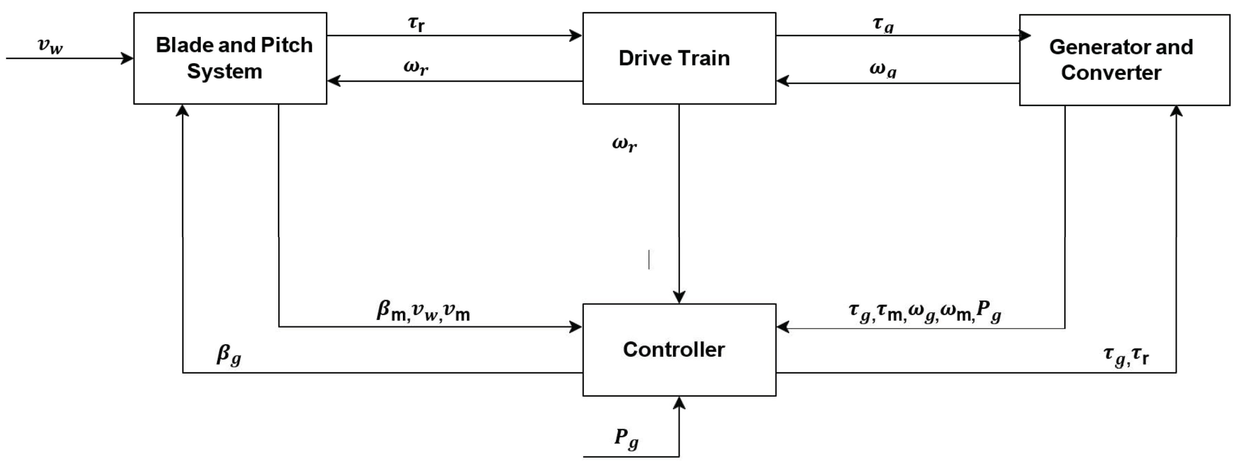
3.1. Mean Components of Wind Turbine

The main components of wind energy are listed below [37] (Figure 1):

• Anemometer for measuring wind speed; the data are controlled by the controller;
• Blades to propel movement by harnessing the power of the wind;
• Brake, used on storm days or in case of maintenance (hydraulically, mechanically, or electrically);
• Controller to control the functions of the turbine (to turn on and shut off the turbine);
• Gear box, connecting the lower speed shaft with the higher one, which increases the speed from 60 rpm to more than 1000 rpm; in some cases, it could reach the 1800 rpm required to generate electricity;
• Generators to produce 60-cycle AC electricity;
• Low-speed shaft, which moves 30 to 60 rpm based on the wind speed;
• A nacelle at the top of the tower, which contains most of the turbine parts (generator, brake, speed shafts, and controller);
• High-speed shaft, which drives the generator;
• Pitch, which increases the turbine efficiency in case of low-speed wind, or decreases the efficiency in extreme cases;
• Rotor, which comprises the blades along with a hub;
• A tower made of concrete or steel, which produces electricity based on its height;
• Wind vane, which indicates the wind direction and passes the data to the yaw system to move the nacelle to face the wind direction;
• Yaw drive, which receives the data from the vane and keeps the blades facing the wind;
• Yaw motor, which supplies the yaw drive with power.

Figure 1 illustrates the subsystems constituting the wind turbine system, including the blade and pitch subsystem, the drive train, the generator, and the converter subsystem. The description of the parameters of the subsystems is presented in

Table 1. Wind turbine water parameters.

Parameter	Description	Parameter	Description
Pr	Rated power	Jg	Generator inertia (high-speed shaft)
α	Empirical wind shear exponent	ηg	Efficiency of generator
H	Hub height	αgc	Generator and converter parameter
R	Radius of rotor	τr	Aerodynamic torque
ρ	Air density	Cq	Torque coefficient
ζ	Damping factor	θ∆	Drive train torsion angle
ωn	Natural frequency	τg	Generator torque
Bdt	Torsion damping coefficient	ωr	Angular speed of the rotor
Kdt	Torsion stiffness	ωg	Angular speed of the generator
Jr	Rotor inertia (low-speed shaft)	λ	Tip speed ratio
Br	Rotor external damping	β	Blade pitch angle
Bg	Generator external damping	vw	Wind speed
ηdt	Drive train efficiency	Pg	Generated power
Ng	Gearbox ratio	vm	Mean wind speed
Tm	Mechanical torque	Te	Electrical torque
ω	Angular velocity	Cp	Power coefficient
θ	Blade angle

[38].

The method of TSR needs the measurement of the wind speed and rotor speed. It is defined as the ratio between the linear speed of the blade tips and the effective speed of the wind [25]:

$$\lambda ={\displaystyle \frac{{\omega }_{r}R}{{\nu }_{\omega }}}$$

(1)

where

λ: the tip speed ratio;

${\nu }_{\omega }$: the wind speed (m/s);

${\omega }_r$: the mechanical angular velocity of the WT rotor.

An anemometer was employed to measure the wind speed, while the rotor speed was determined using sensors mounted on the turbine’s rotor shaft. The anemometer data are fed to the turbine controller, which processes this information along with the rotor speed to continuously calculate TSR. This accurate measurement and control are essential for the effective implementation of the TSR method, which aims to maintain the wind turbine’s operation at its optimal TSR to maximize energy extraction. By integrating these sensors and control mechanisms, the study ensures the precise and reliable operation of the WECS, leading to efficient power extraction.

The efficiency of the MPPT of a wind turbine is likely to be improved by applying the fractional order PID based on the tip speed ratio (TSR). Fractional order proportional integral derivative (FOPID) could be considered an advanced controller of the PID controller. The following equation presents the time domain equation for the FOPID controller with related error for the closed-loop system [39]:

$$y\left(t\right)=K_{p}e\left(t\right)+K_i{I}_t^{\mu }e\left(t\right)+K_d{D}_t^{\alpha }e\left(t\right)$$

(2)

where

e(t): the error between the reference and recorded value;

y(t): the controller response based on the calculated error.

Using the Laplace transform theory on Equation (2):

$$Y\left(s\right)=K_p\mathrm{E}\left(s\right)+K_i{s}^{-\mu }\mathrm{E}\left(s\right)+K_d{s}^{\alpha }\mathrm{E}\left(s\right)$$

(3)

By taking the E(s) as a common factor, Equation (3) can be written as:

$$Y\left(s\right)=\mathrm{E}\left(s\right)\left[K_p+K_i{s}^{-\mu }+K_d{s}^{\alpha }\right]$$

(4)

In this case, the transfer function of FOPID can be presented as:

$$G\left(s\right)={\displaystyle \frac{Y\left(s\right)}{\mathrm{E}\left(s\right)}}=\left[K_p+K_i{s}^{-\mu }+K_d{s}^{\alpha }\right]$$

(5)

Figure 2 shows the block diagram for the FOPID controller.

Using Laplace transfer, the transfer function is:

$$s{e}_{\omega }\left(s\right)-e_{\omega }\left(0\right)=-{\displaystyle \frac{k_i}{k_p}}{\displaystyle \frac{1}{s^{\mu -1}}}{e}_{\omega }\left(s\right)$$

(6)

where s is the Laplace operator; $e_{\omega }\left(s\right)$ is the Laplace transform of ${\epsilon }_{\omega }\left(t\right)$; and $e_{\omega }\left(0\right)$ is the initial condition of ${\epsilon }_{\omega }$.

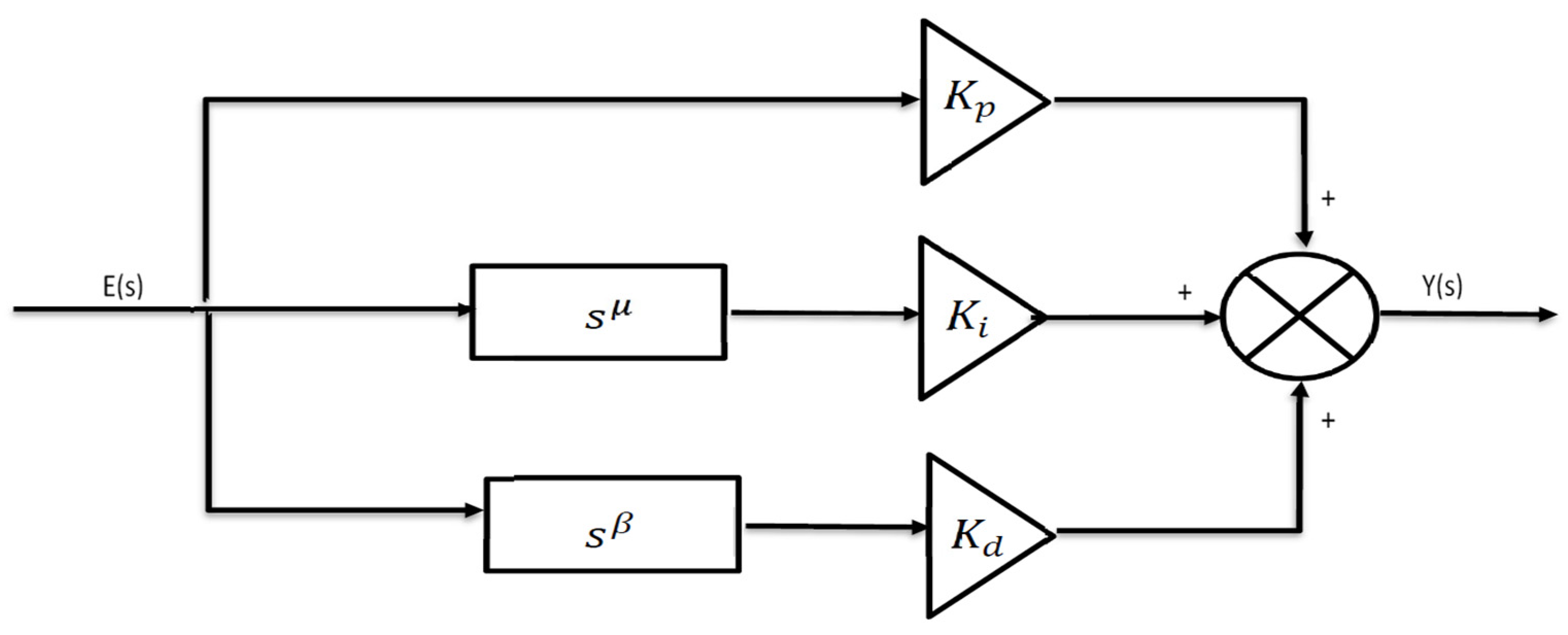
3.2. Fractional Order Slide Mode Control FOPI SMC_P$I^{\mu }$

The solution proposed by the previous study of Santi et al. [40] has also been adopted in the present study. The solution is the addition of integral error to the control law to obtain zero error, as shown below:

$$S_{\omega }=k_p\left({\epsilon }_{\omega }\right)+k_i\int {\epsilon }_{\omega }$$

(7)

where $k_p{, k}_i$ are proportional and integral parameters of the fractional order sliding mode control.

The fractional order integral is used as a sliding surface to improve this method. In this case, the P$I^{\mu }$ controller can be stated as:

$$S_{\omega }=k_p\left({\epsilon }_{\omega }\right)+k_i{I}^{\mu }\left({\epsilon }_{\omega }\right)$$

(8)

where $k_p,{ k}_i,\mu$ are parameters of the surface to be determined. The deriving of the previous equation $S_{\omega }$ can be carried out as follows:

$${\dot{S}}_{\omega }=k_p{\dot{\epsilon }}_{\omega }+K_i{I}^{\mu -1}\left({\epsilon }_{\omega }\right)$$

(9)

Based on the turbine model and the sliding mode surface, the derivative of the sliding surface is calculated as follows:

$${\dot{S}}_{\omega }={\dot{\epsilon }}_{\omega }={\dot{\omega }}_{ref}-{\dot{\omega }}_r$$

(10)

$${\dot{\omega }}_r={\displaystyle \frac{1}{J_t}}\left(T_a-K_t{\omega }_r-T_g\right)$$

(11)

By using (10) and (11), the following equation is achieved:

$${\dot{S}}_{\omega }={\dot{\epsilon }}_{\omega }={\dot{\omega }}_{ref}-{\displaystyle \frac{1}{J_t}}\left(T_a-K_t{\omega }_r-T_g\right)$$

(12)

The use of the concept of the fractional-order integral is supported to enhance this method. The ${PI}^u$ controller as a sliding surface structure can be determined as follows:

$${\dot{S}}_{\omega }=k_p{\dot{\epsilon }}_{\omega }+K_i{I}^{\mu -1}\left({\epsilon }_{\omega }\right)$$

(13)

$$T_g=T_{geq}+T_{gdisc}$$

(14)

where $T_{gdisc}$: the discontinuous component; $T_{geq}$: the continuous component.

To clarify, Ueg represents the equivalent control input in the context of sliding mode control. It is derived as the continuous part of the total control input, T_g, and is essential for maintaining the system on the sliding surface.

Substituting (13) for (14), the following equation is achieved:

$${\dot{S}}_{\omega }={\dot{\epsilon }}_{\omega }={\dot{\omega }}_{ref}-{\displaystyle \frac{1}{J_t}}(T_a-K_t{\omega }_r-\left(T_{geq}+T_{gdisc}\right))$$

(15)

Equation (15) can be substituted to (13), to obtain the following:

$${\dot{S}}_{\omega }=k_p\left[{\dot{\omega }}_{ref}-{\displaystyle \frac{1}{J_t}}(T_a-K_t{\omega }_r-T_{geq}-T_{gdisc})\right]+K_i{I}^{\mu -1}({\omega }_{ref}-{\omega }_r)$$

(16)

$${\displaystyle \frac{1}{k_p}}{\dot{S}}_{\omega }={\dot{\omega }}_{ref}-{\displaystyle \frac{1}{J_t}}(T_a-K_t{\omega }_r-T_{geq}-T_{gdisc})+{\displaystyle \frac{k_i}{k_p}}{I}^{\mu -1}({\omega }_{ref}-{\omega }_r)$$

(17)

$${\displaystyle \frac{J_t}{k_p}}{\dot{S}}_{\omega }=J_t{\dot{\omega }}_{ref}-(T_a-K_t{\omega }_r-T_{geq}-T_{gdisc})+J_t{\displaystyle \frac{k_i}{k_p}}{I}^{\mu -1}({\omega }_{ref}-{\omega }_r)$$

(18)

$${\displaystyle \frac{J_t}{k_p}}{\dot{S}}_{\omega }=-T_a+K_t{\omega }_r+T_{geq}+T_{gdisc}+J_t\left[{\dot{\omega }}_{ref}+{\displaystyle \frac{k_i}{k_p}}{I}^{\mu -1}\left({\omega }_{ref}-{\omega }_r\right)\right]$$

(19)

However, the following equation is achieved after applying SMC during the steady state [41]:

$$S_{\omega }=0,{\dot{S}}_{\omega }=0,T_{gdisc}=0$$

(20)

Due to the inherent nature of discontinuous control in sliding mode, T_gdisc can exhibit chattering, which refers to high-frequency oscillations around the sliding surface. These oscillations, though minimized by techniques such as boundary layer design and higher order sliding modes, cannot be eliminated, and hence T_gdisc might not be exactly zero in practical implementations. This chattering can affect the performance and stability of the control system, necessitating further measures to mitigate its impact.

By substitution, the following equivalent controller is achieved:

$$0=-T_a+K_t{\omega }_r+T_{geq}+J_t\left[{\dot{\omega }}_{ref}+{\displaystyle \frac{k_i}{k_p}}{I}^{\mu -1}\left({\omega }_{ref}-{\omega }_r\right)\right]$$

(21)

$$-T_{geq}=-T_a+K_t{\omega }_r+J_t\left[{\dot{\omega }}_{ref}+{\displaystyle \frac{k_i}{k_p}}{I}^{\mu -1}\left({\omega }_{ref}-{\omega }_r\right)\right]$$

(22)

$$T_{geq}=\left(T_a-K_t{\omega }_r\right)-J_t\left[{\dot{\omega }}_{ref}+{\displaystyle \frac{k_i}{k_p}}{I}^{\mu -1}\left({\omega }_{ref}-{\omega }_r\right)\right]$$

(23)

But by definition, the control signal $U_{eg}$ is equal to $T_{geq}$, so:

$$U_{eg}=\left(T_a-K_t{\omega }_r\right)-J_t\left[{\dot{\omega }}_{ref}+{\displaystyle \frac{k_i}{k_p}}{I}^{\mu -1}\left({\omega }_{ref}-{\omega }_r\right)\right]$$

(24)

In this study, we apply both sliding mode control and fractional-order control to achieve the robust and precise control of the wind energy conversion system [42,43].

3.3. Controller Optimization for FOPID Using PSO

The PSO algorithm was specifically adapted for tuning fractional-order controllers, as detailed in the literature by Timis et al. [44]. The PSO algorithm initializes a swarm of particles, each representing a potential solution in the search space, and iteratively updates their positions based on personal and global best experiences. This optimization technique is well suited for the FO-PID controllers due to its ability to handle nonlinearities and complex search spaces. The application of PSO to FOPID controllers introduces additional complexity due to the presence of fractional-order integrals and derivatives, which necessitate careful approximation and handling. The iterative equations governing the PSO process are defined as follows [45]:

$$V_{iD}^{t+1}=K\times V_{iD}^t+c_1{r}_1\left(P_{iD}^t-X_{iD}^t\right)+c_2{r}_2\left(G_{iD}^t-X_{iD}^t\right)$$

(25)

$$X_{iD}^{t+1}=V_{iD}^{t+1}+X_{iD}^t$$

(26)

where

$i=1,\dots ,n$ and n is the size of the swarm;

D is the dimension of space;

$c_1,c_2$ are positive constants;

K is inertia;

$r_1,r_2$ are random numbers;

$t$ is the iteration number;

P is the best previous position;

G is the best individual among all members in the swarm.

The specific cost function we employed focuses on minimizing the following:

• Tracking Error: The deviation of the system output from the desired reference trajectory.
• Control Effort: The magnitude of the control signals, to ensure that they are within practical limits.
• Robustness: The ability of the controller to maintain performance in the presence of disturbances and model uncertainties.

The optimized cost function for the fractional order controller is thus:

$$J=w_1\cdot \left({\displaystyle \frac{1}{T}}{\int }_0^{T}e{\left(t\right)}^2\hspace{0.17em}dt\right)+w_2\cdot \left({\displaystyle \frac{1}{T}}{\int }_0^{T}u{\left(t\right)}^2\hspace{0.17em}dt\right)+w_3\cdot \sum _{j=1}^M\left|{\displaystyle \frac{d\varphi \left(j\right)}{dj}}\right|$$

where e(t) is the tracking error at time t, w are the weights assigned to different performance criteria, u(t) is the control effort at the time, ϕ(j) represents the system response characteristics used to evaluate robustness, T is the total time duration considered, and M is the number of disturbance scenarios evaluated.

The steps of the algorithm of particle swarm optimization are stated below [41,45]:

• Initialization: An array of particles with random positions and velocities is created.
• Fitness Evaluation: Each particle’s fitness value is evaluated according to the desired optimization function.
• Update Best Positions: The algorithm updates the personal best $P_{best}$ and global best $G_{best}$ positions based on the current fitness evaluations.
• Update Velocities and Positions: The velocities and positions of the particles are updated using the iterative equations.
• Iteration: Steps 2–4 are repeated until the stopping criterion is met, typically based on the number of iterations or a convergence threshold.

This method has shown effectiveness in optimizing the parameters of FO-PID controllers, enhancing their performance in dynamic and nonlinear systems.

4. Results

The wind that rotates the blades determines the output energy of the wind turbine. Simulations of the wind speed profile were conducted as time series data, ranging from a minimum of 6.711 m/s to a maximum of 13.19 m/s, illustrating the varying wind conditions over time. The average wind speed recorded stood at 10.08 m/s. Figure 3 depicts the wind speed profile over a 50-s interval. This profile forms the basis for understanding the wind turbine’s performance at different speeds.

4.1. Maximum Power of Wind Turbine

Operating a wind turbine at the maximum power coefficient (β = β_min = 2) yields the highest power output from the turbine. The generator torque substantiates the relationship between the turbine’s operation at this coefficient and the resultant torque generated.

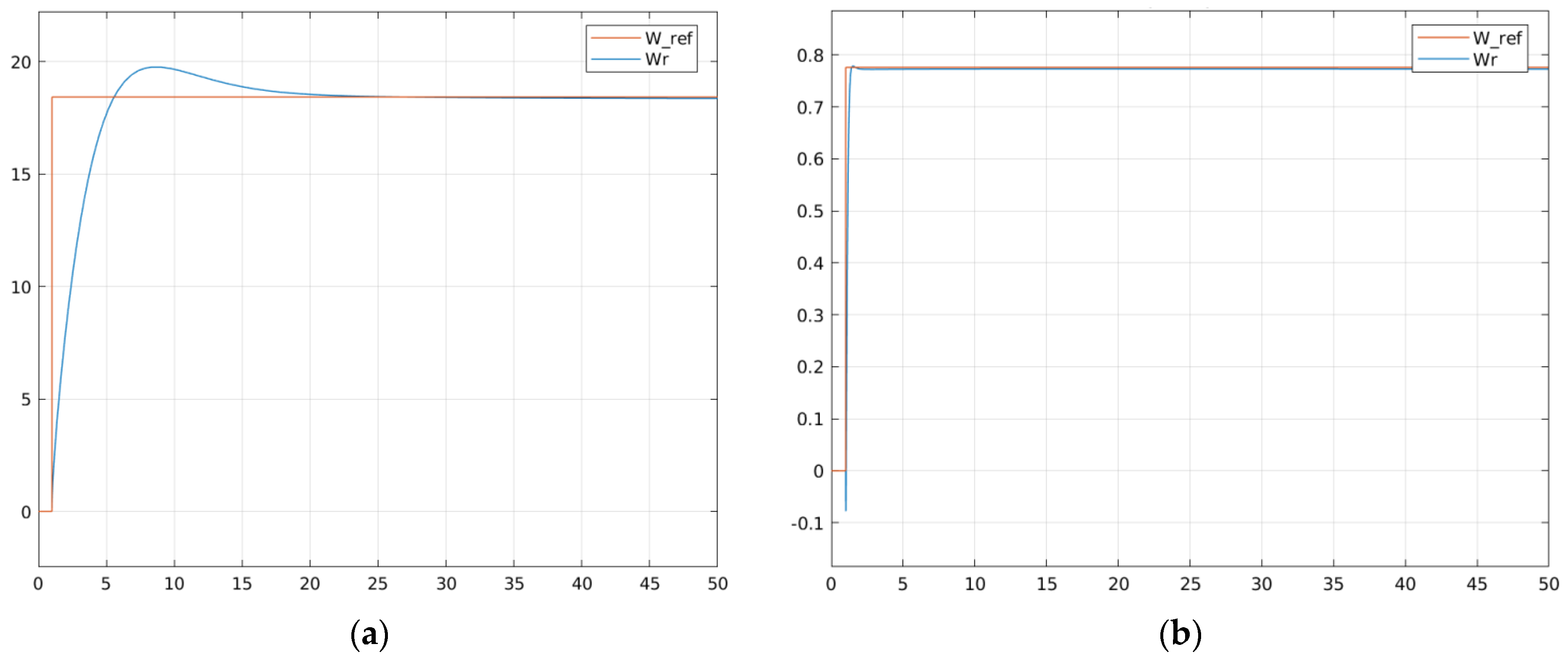
4.2. Response of Controllers with PSO

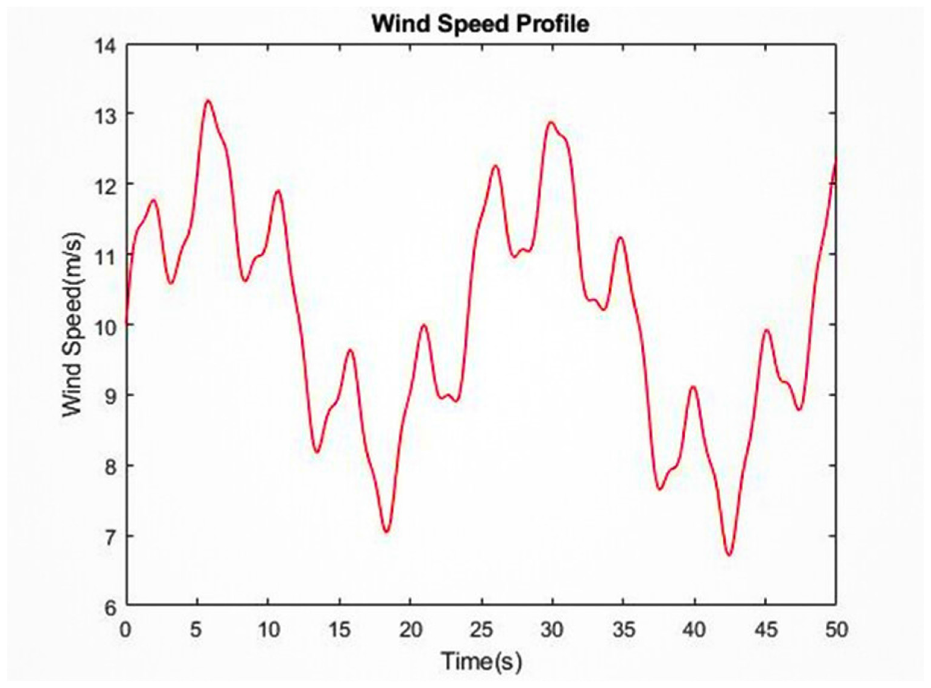
The system was integrated with the PSO method to enhance the parameters of various controllers.

Table 2. Optimized parameters for FOPID and FOPID-SMC.

	FOPID-Controller	FOPID-SMC
Kp	0.39138	0.83778
Ki	0.73452	0.01
Lambda	0.80659	0.01
Kd	0.01962	0.65638
Mu	0.6882	0.9234

outlines the optimized parameters for the FOPID and FOPID-SMC achieved through PSO. The traditional PID controller is not a good choice for the MPPT of wind turbines due to the nonlinearity behavior of wind turbines, considering the step response. The FOPID controller has an advantage based on settling time and steady-state error, although there is a tradeoff between FOPI_SMC and FOPID_SMC.

Figure 4 depicts the step response of the wind turbine under two different controllers—FOPID and FOPID-SMC—optimized using the PSO method. FOPID-SMC exhibits faster rise times and reduced overshoot compared to the FOPID controller. This suggests that the FOPID-SMC algorithm better tracks the desired setpoints, ensuring quicker convergence to optimal operating conditions and minimizing deviations from the desired values.

Table 3. Comparison between different controllers with optimization.

Time Domain	Without Controller	PID	FOPID	Basic Sliding Mode Control	FOPI–Sliding Mode Control	FOPID–Sliding Mode Control
Rise Times (s)	10.1620	4.3681	3.0966	0.2105	0.2173	0.2262
Settling Time (s)	19.1035	28.9442	37.39	1.3753	1.4126	1.3468
Peak Overshoot (%)	0	7.6399	46	0.0087	0.0442	1.7527
Steady-State Error	1.5981	0.0361	0.0022	4.9342 × 10−4	0.0029	3.5838 × 10−4

presents a comparative analysis of different controllers in terms of key performance metrics. In the context of rise times (s), both the FO-based controllers, FOPI–Sliding Mode Control and FOPID–Sliding Mode Control, along with the Basic Sliding Mode Control, exhibit significantly lower rise times compared to the IO (PID) controller. Notably, the proposed FOPID–Sliding Mode Control showcases remarkably faster response times, signifying its superiority over the IO (PID) controller in achieving quicker system responses. Analyzing steady-state error, all FO-based controls display superior performance in maintaining output accuracy compared to the IO (PID) controller. Particularly, the proposed FOPID–Sliding Mode Control demonstrates the lowest steady-state error among other methods, indicating its enhanced precision in reaching and sustaining the desired output. Therefore, these results confirm the superiority of the proposed FOPID–Sliding Mode Control method over the IO (PID) controller in terms of both response speed and accuracy in maintaining the desired output, showcasing its potential for improved control precision and faster system responses.

4.3. Wind Profile

The proposed controllers were applied to the WECS. The generator speed response was considered, which is directly related to the studied method of TSR to achieve MPPT. The studied wind velocity profile had a mean of 10.08 m/s value, as shown in Figure 5a. Figure 5b–d show the generator speed response of wind turbines without a controller, with a PID controller, and with a FOPID controller, respectively. Figure 5 shows that there are significant differences between the rotor speed (ω_r) and the reference speed (ω_ref) in all three cases. Figure 5b shows that the absence of a controller leads to a highly erratic rotor speed (ωr_r) that fails to follow the reference speed (ω_ref). This discrepancy is due to the lack of any regulating mechanism to counteract the fluctuations in wind speed, resulting in poor tracking performance and inefficiency in power extraction. Figure 5c shows that the introduction of a PID controller improves the tracking of ω_ref by ω_r. However, there are still notable deviations, especially during transient states. The PID controller, while effective to some extent, struggles to cope with rapid changes in wind speed due to its inherent limitations in handling nonlinearities and high-frequency disturbances, resulting in a compromise in achieving MPPT. On the other hand, Figure 5d shows that the FOPID controller further enhances the tracking capability, reducing the gap between ω_r and ω_ref. The fractional-order component of the FOPID controller allows for a more flexible and robust response, adapting better to the dynamics of the wind turbine system. However, despite these improvements, perfect tracking is not achieved, indicating room for further optimization. The deviations, although smaller, are still present and could be attributed to factors such as parameter tuning and the inherent complexity of the wind turbine dynamics. The progression from no controller to PID, and then to FOPID, demonstrates an incremental performance improvement. However, the persistent discrepancies suggest that additional measures, possibly involving more sophisticated algorithms or hybrid control approaches, are necessary to achieve optimal MPPT and system stability.

The tip speed ratio required the measurement of the wind speed and rotor speed that will help in determining optimal TSR. Figure 6a,b show the response of the power coefficient using FOPI-SMC without disturbance and the zoom of the power coefficient for FOPI-SMC, respectively. It depicts a good capability of tracking as compared to the traditional SMC. Further, Figure 6c illustrates the sliding surface response, depicting a good capability of tracking by removing high-frequency oscillations. Figure 6d shows the generator speeds with FOPI-SMC, while Figure 6e shows the wind profile response of the wind turbine with FOPI-SMC.

Figure 7a,b show the response of the power coefficient using FOPID-SMC without disturbance and the zoom of the power coefficient for FOPID-SMC, respectively. It depicts a good capability of tracking as compared to the traditional SMC. Further, Figure 7c illustrates the sliding surface response, depicting a good capability of tracking by removing high-frequency oscillations. Figure 7d shows the generator speeds with FOPID-SMC, while Figure 7e shows the wind profile response of the wind turbine with FOPID-SMC and Figure 7f shows the control signal T_g without disturbance.

Figure 5, Figure 6 and Figure 7 illustrate the responses of the wind turbine system under different control strategies (without a controller, with PID, and with FOPID controllers) in correlation with the wind speed profile. The analysis of these figures demonstrates that the FOPID controller significantly reduces steady-state errors compared to the PID controller, showcasing its superior ability to adjust the generator speeds to match the varying wind speeds more accurately.

4.4. Response of Controllers with Disturbance and PSO

A disturbance to the system was added exactly to the output of the regulator to simulate the real case, as shown in Figure 8a. The shape of the introduced disturbance is illustrated in Figure 8b.

The introduction of disturbance to the system for FOPI-SMC is illustrated in Figure 9. Figure 10a,b show the response of power coefficient using FOPI-SMC with disturbance and zoom for power coefficient at the three areas of disturbance, respectively.

The sliding surface for FOPI SMC is shown in Figure 11a. Figure 11b,c show the zoom for the sliding surface of FOPI-SMC and zoom for the sliding surface of FOPI-SMC at the three areas of disturbance, respectively.

Figure 12 shows the generator speed for FOPI SMC with disturbance. The zoom for the generator speed of FOPI SMC at the three areas of disturbance is illustrated in Figure 13a–c.

The wind profile of the wind turbine with FOPI SMC and disturbance is shown in Figure 14.

Figure 8, Figure 9, Figure 10, Figure 11, Figure 12, Figure 13 and Figure 14 exhibit the impact of disturbances on FOPI-SMC. The introduction of disturbances affects the power coefficient, sliding surface, generator speed, and wind profile. The analysis reveals that FOPI-SMC effectively tracks the power coefficient and exhibits a more stable response compared to the disturbance, indicating robustness in handling external disruptions.

The introduction of disturbance to the system for FOPID-SMC is illustrated in Figure 15.

The response of the power coefficient FOPID-SMC with the existence of disturbance, zoom for the power coefficient FOPID-SMC response with disturbance, and zoom power coefficient FOPID-SMC at the three areas of disturbance are illustrated in Figure 16a–c.

The behavior of sliding surfaces under the disturbance effect was also studied. The response of the sliding surface under the disturbance effect is shown in Figure 17a. The zoom of the sliding surface at the three areas of disturbance and for each area of disturbance is shown in Figure 17b,c, respectively.

Figure 18a illustrates the generator speed for FOPID-SMC with disturbance, while Figure 18b illustrates the zoom for the generator speed of FOPID-SMC at the three areas of disturbance. The wind profile of the wind turbine with FOPID-SMC and disturbance is shown in Figure 19.

Figure 15, Figure 16, Figure 17, Figure 18 and Figure 19 demonstrate the behavior of the wind turbine system controlled by the FOPID-SMC algorithm under disturbances. The responses of the power coefficient, sliding surface, generator speed, and wind profile show that the FOPID-SMC effectively mitigates the effects of disturbances, maintaining stable performance and accurately tracking the desired setpoints even in the presence of disruptions.

4.5. Wind Profile Disturbance and Sensor Noise-FOPID SMC with OPT Optimization

Figure 20a portrays the introduced sensor noise, replicating real-world scenarios where sensor irregularities or external disturbances influence the wind turbine system. This visualization showcases fluctuations or deviations in the sensor data, potentially mimicking environmental interferences or inaccuracies in measurements. On the other hand, Figure 20b illustrates the wind profile under the influence of sensor noise when the wind turbine system operates with the FOPID-SMC algorithm. These figures collectively demonstrate the consequential impact of sensor noise on the wind turbine’s behavior and how effectively the FOPID-SMC algorithm manages these disturbances. Through this comparison, it becomes evident how the introduced sensor noise influences the wind profile and how adeptly the FOPID-SMC algorithm responds to and mitigates these disturbances, elucidating its stability and resilience in addressing real-world operational challenges.

5. Conclusions

In conclusion, the proposed FOPID-SMC algorithm has an advantage in its capability for tracking the maximum peak power points. The behaviors of the two combination algorithms (FOPI-SMC and FOPID-SMC) were found to depict good and ability tracking behavior; however, the FOPID-SMC algorithm showed the greatest advantage as compared to FOPI-SMC because it provides good tracking reference, reduces overshoot, and suppresses the phenomenon of chattering. The proposed control algorithm (FOPID-SMC) shows robustness and effectiveness to uncertainty parameters and external changeable disturbance.

The present study has certain limitations regarding the availability of comprehensive datasets and real-time monitoring capabilities, despite the potential value of analyzing the evolution of the control input T_g to ascertain its stability and mitigate any chattering phenomena. The absence of this analysis may limit the depth of insight into the system’s behavior under specific operational conditions. Addressing this limitation through further empirical studies or advanced data acquisition methodologies could offer a better understanding of the control system dynamics and enhance the robustness of its implementation in practical scenarios.

References

1. Benbouhenni, H.; Boudjema, Z.; Bizon, N.; Thounthong, P.; Takorabet, N. Direct power control based on modified sliding mode controller for a variable-speed multi-rotor wind turbine system using PWM strategy. Energies 2022, 15, 3689. [Google Scholar] [CrossRef]
2. Shchur, I.; Klymko, V.; Xie, S.; Schmidt, D. Design features and numerical investigation of counter-rotating VAWT with co-axial rotors displaced from each other along the axis of rotation. Energies 2023, 16, 4493. [Google Scholar] [CrossRef]
3. Benbouhenni, H.; Bizon, N. A new direct power control method of the DFIG-DRWT system using neural PI controllers and a four-level neural modified SVM technique. J. Appl. Res. Technol. 2023, 1, 36–55. [Google Scholar] [CrossRef]
4. REN21. Renewable Global Status Report. 2020. Available online: https://www.ren21.net/reports/global-status-report/ (accessed on 23 March 2024).
5. Chauhan, S.; Sameeullah, M.; Dahiya, R. Maximum Power Point Tracking scheme for variable speed wind generator. In Proceedings of the IEEE 6th India International Conference on Power Electronics (IICPE), Kurukshetra, India, 8–10 December 2014. [Google Scholar]
6. Thongam, J.S.; Ouhrouche, M. MPPT control methods in wind energy conversion systems. Fundam. Adv. Top. Wind. Power 2011, 15, 339–360. [Google Scholar]
7. Bougdour, S.; Elhouti, R.; Sefriti, S.; Boumhidi, I. Optimal predictive control model of wind turbine. In Proceedings of the 2021 Fifth International Conference on Intelligent Computing in Data Sciences (ICDS), Virtual, 20–22 October 2021; pp. 1–7. [Google Scholar]
8. Ali, K.-M.; Barambones, O. Higher Order Sliding Mode Control of MIMO Induction Motors: A New Adaptive Approach. Mathematics 2023, 11, 4558. [Google Scholar] [CrossRef]
9. Hu, L.; Xue, F.; Qin, Z.; Shi, J.; Qiao, W.; Yang, W.; Yang, T. Sliding mode extremum seeking control based on improved invasive weed optimization for MPPT in wind energy conversion system. Appl. Energy 2019, 248, 567–575. [Google Scholar] [CrossRef]
10. Kazmi, S.M.; Goto, H.; Guo, H.J. Review and critical analysis of the research papers published to date on maximum power point tracking in wind energy conversion system. In Proceedings of the IEEE Energy Conversion Congress and Exposition, Atlanta, GA, USA, 12–16 September 2010; pp. 4075–4082. [Google Scholar]
11. Liu, J.; Meng, H.; Hu, Y.; Lin, Z.; Wang, W. A novel MPPT method for enhancing energy conversion efficiency taking power smoothing into account. Energy Convers. Manag. 2015, 101, 738–748. [Google Scholar] [CrossRef]
12. Cao, A.; Cen, L.; Chen, J. Optimal Torque Control for Large-Scale Wind Turbine Systems Based on Sliding Mode Control. In Proceedings of the 2018 37th Chinese Control Conference (CCC), Wuhan, China, 25–27 July 2018. [Google Scholar]
13. Liu, D.; Xia, Y.; Li, R.; Liu, P. Integral sliding mode control of low-speed wind turbine. In Proceedings of the 2019 Chinese Automation Congress (CAC), Hangzhou, China, 22–24 November 2019. [Google Scholar]
14. Maati, Y.A.E.; Bahir, L.E. Optimal Fault Tolerant Control of Large-Scale Wind Turbines in the Case of the Pitch Actuator Partial Faults. Complexity 2020, 2020, 1–17. [Google Scholar] [CrossRef]
15. Van, T.L.; Nguyen, D.Q.; Duy, V.H.; Nguyen, H. Fast Maximum Power Point Tracking Control for Variable Speed Wind Turbines. In Proceedings of the International Conference on Advanced Engineering Theory and Applications, Ho Chi Minh, Vietnam, 7–9 December 2017; pp. 821–829. [Google Scholar]
16. Porate, D.K.; Gawande, S.; Munshi, A.; Porate, K.; Kadwane, S.; Waghmare, M. Zero Direct-axis Current (ZDC) Control for Variable Speed Wind Energy Conversion System using PMSG. Energy Procedia 2017, 117, 943–950. [Google Scholar] [CrossRef]
17. Kumar, S.S.; Jayanthi, K.; Kumar, N.S. Maximum power point tracking for a PMSG-based variable speed wind energy conversion system using optimal torque control. In Proceedings of the 2016 International Conference on Advanced Communication Control and Computing Technologies (ICACCCT), Ramanathapuram, India, 25–27 May 2016; pp. 347–352. [Google Scholar]
18. Khiabani, A.G.; Heydari, A. Optimal torque control of permanent magnet synchronous motors using adaptive dynamic programming. IET Power Electron. 2020, 13, 2442–2449. [Google Scholar] [CrossRef]
19. Karabacak, M.; Fernandez-Ramirez, L.M.; Kamal, T. A new hill climbing maximum power tracking control for wind turbines with inertial effect compensation. IEEE Trans. Ind. Electron. 2019, 66, 8545–8556. [Google Scholar] [CrossRef]
20. Dida, A.; Attous, D.B. Adaptive hill-climb searching method for MPPT algorithm based DFIG system using fuzzy logic controller. Int. J. Syst. Assur. Eng. Manag. 2017, 8, 424–434. [Google Scholar] [CrossRef]
21. Yaakoubi, A.; Amhaimar, L.; Attari, K.; Harrak, M.; Halaoui, M.; Asselman, A. Non-linear and intelligent maximum power point tracking strategies for small size wind turbines: Performance analysis and comparison. Energy Rep. 2019, 5, 545–554. [Google Scholar] [CrossRef]
22. Tan, K.; Islam, S. Optimum control strategies in energy conversion of PMSG wind turbine system without mechanical sensors. IEEE Trans. Energy Convers. 2004, 19, 392–399. [Google Scholar] [CrossRef]
23. Camblong, J.; Vechiu, I.; Guillaud, X.; Etxeberria, A.; Kreckelbergh, S. Wind turbine controller comparison on an island grid in terms of frequency control and mechanical stress. Renew. Energy 2014, 63, 37–45. [Google Scholar] [CrossRef]
24. Oliveira, M.M.; Grigoletto, F.B. Fuzzy Sensorless MPPT Strategy for Small Wind Turbines. In Proceedings of the 2019 IEEE PES Innovative Smart Grid Technologies Conference-Latin America (ISGT Latin America), Gramado, Brazil, 15–18 September 2019. [Google Scholar]
25. Ardjal, A.; Mansouri, R.; Bettayeb, M. Fractional sliding mode control of wind turbine for maximum power point tracking. Trans. Inst. Meas. Control 2019, 41, 447–457. [Google Scholar] [CrossRef]
26. Barambones, O. Sliding Mode Control Strategy for Wind Turbine Power Maximization. Energies 2012, 5, 2310–2330. [Google Scholar] [CrossRef]
27. Mahdavian, M.; Wattanapongsakorn, N.; Shahgholian, G.; Mozafarpoor, S.H.; Janghorbani, M.; Shariatmadar, S.M. Maximum power point tracking in wind energy conversion systems using tracking control system based on fuzzy controller. In Proceedings of the Electrical Engineering/Electronics, Computer, Telecommunications and Information Technology (ECTI-CON), 2014 11th International Conference, Nakhon Ratchasima, Thailand, 14–17 May 2014. [Google Scholar]
28. Salim, O.M.; Zohdy, M.A.; Abdel-Aty-Zohdy, H.; Dorrah, H.T.; Kamel, A.M. Type-2 fuzzy logic pitch controller for wind turbine rotor blades. In Proceedings of the 2011 IEEE National Aerospace and Electronics Conference (NAECON), Dayton, OH, USA, 20–22 July 2011. [Google Scholar]
29. Li, Y.; Chengxin, L. Overview of Maximum Power Point Tracking Control Method for Wind Power Generation System. IOP Conf. Ser. Mater. Sci. Eng. 2018, 428, 12007. [Google Scholar] [CrossRef]
30. Sitharthan, R.; Parthasarathy, T.; Sheeba Rani, S. An improved radial basis function neural network control strategy-based maximum power point tracking controller for wind power generation system. Trans. Inst. Meas. Control 2019, 41, 3158–3170. [Google Scholar] [CrossRef]
31. Sitharthan, R.; Karthikeyan, M.; Sundar, D.S. Adaptive hybrid intelligent MPPT controller to approximate effectual wind speed and optimal rotor speed of variable speed wind turbine. ISA Trans. 2020, 96, 479–489. [Google Scholar] [CrossRef]
32. Fathy, A.; El-baksawi, O. Grasshopper optimization algorithm for extracting maximum power from wind turbine installed in Al-Jouf region. J. Renew. Sustain. Energy 2019, 11, 033303. [Google Scholar] [CrossRef]
33. Li, B.X.; Zhao, X.F.; Liu, Y.W.; Zhao, X.; Robust, H. Control of fractional-order switched systems with order 0 < α < 2 and uncertainty. Fractal Fract. 2022, 6, 164. [Google Scholar]
34. Wang, J.; Liu, Y.; Wu, H.Y.; Lu, S.; Zhou, M. Ensemble FARIMA prediction with stable infinite variance innovations for supermarket energy consumption. Fractal Fract. 2022, 6, 276. [Google Scholar] [CrossRef]
35. Jia, T.Y.; Chen, X.Y.; He, L.P.; Zhao, F.; Qiu, J.L. Finite-time synchronization of uncertain fractional-order delayed memristive neural networks via adaptive sliding mode control and its application. Fractal Fract. 2022, 6, 502. [Google Scholar] [CrossRef]
36. Zhang, X.F.; Dai, L.W. Image enhancement based on rough set and fractional order differentiator. Fractal Fract. 2022, 6, 214. [Google Scholar] [CrossRef]
37. MWPS Powering the World. 2019. Available online: https://www.mwps.world/2011/07/27/inside-wind-turbine/ (accessed on 23 March 2024).
38. Odgaard, P.F.; Stoustrup, J.; Kinnaert, M. Fault-tolerant control of wind turbines: A benchmark model. IEEE Trans. Control. Syst. Technol. 2013, 21, 1168–1182. [Google Scholar] [CrossRef]
39. Mukhtar, A.; Tiwari, P.M.; Singh, H.P. Performance Improvement of Wind Turbine Control using Fractional Order PID Controller with PSO Optimized gains. In Proceedings of the International Conference on Advances in Computing, Communication & Materials (ICACCM), Dehradun, India, 10–11 November 2020; pp. 374–379. [Google Scholar]
40. Santi, E.; Monti, A.; Li, D. Synergetic control for DC-DC boost converter: Implementation options. IEEE Trans. Ind. Appl. 2003, 39, 1803–1813. [Google Scholar] [CrossRef]
41. Adhikary, N.; Mahanta, C. Integral backstepping sliding mode control for underactuated systems: Swing-up and stabilization of the Cart–Pendulum System. ISA Trans. 2013, 52, 870–880. [Google Scholar] [CrossRef] [PubMed]
42. Slotine, J.J.; Li, W. Applied Nonlinear Control; Prentice Hall: Englewood Cliffs, NJ, USA, 1991. [Google Scholar]
43. Podlubny, I. Fractional Differential Equations: An Introduction to Fractional Derivatives, Fractional Differential Equations, to Methods of Their Solution and Some of Their Applications; Academic Press: San Diego, CA, USA, 1998. [Google Scholar]
44. Timis, D.D.; Muresan, C.I.; Dulf, E.H. Design and experimental results of an adaptive fractional-order controller for a quadrotor. Fractal Fract. 2022, 6, 204. [Google Scholar] [CrossRef]
45. Kahla, S.; Soufi, Y.; Sedraoui, M. On-off control-based particle swarm optimization for maximum power point tracking of a wind turbine equipped by DFIG connected to the grid with energy storage. Int. J. Hydrogen Energy 2015, 40, 13749–13758. [Google Scholar] [CrossRef]
Figure 1. Wind turbine subsystem block diagram.
Fractalfract 08 00447 g001
Figure 2. FOPID block diagram.
Fractalfract 08 00447 g002
Figure 3. Profile of wind speed.
Fractalfract 08 00447 g003
Figure 4. Step response of wind turbine (a) with FOPID controller; (b) with FOPID Sliding Mode controller.
Fractalfract 08 00447 g004
Figure 5. (a) Wind speed profile; (b) without controller; (c) with PID controller; (d) with FOPID controller.
Fractalfract 08 00447 g005
Figure 6. (a) Power coefficient FOPI-SMC without disturbance; (b) zoom power coefficient FOPI-SMC without disturbance; (c) sliding surface FOPI SMC; (d) generator speed with FOPI SMC without disturbance; (e) wind profile of wind turbine with FOPI-SMC.
Fractalfract 08 00447 g006
Figure 7. (a) Power coefficient FOPID-SMC without disturbance; (b) zoom power coefficient FOPID-SMC without disturbance; (c) sliding surface FOPID-SMC; (d) generator speed with FOPID-SMC without disturbance; (e) wind profile response of the wind turbine; (f) the control signal T_g without disturbance.
Fractalfract 08 00447 g007
Figure 8. (a) Wind turbine along with disturbance; (b) disturbance shape.
Fractalfract 08 00447 g008
Figure 9. Disturbance to the system for FOPI SMC.
Fractalfract 08 00447 g009
Figure 10. (a) Power coefficient FOPI-SMC with disturbance; (b) zoom of power coefficient FOPI SMC with a disturbance.
Fractalfract 08 00447 g010
Figure 11. (a) Sliding surface FOPI-SMC with disturbance; (b) zoom sliding surface FOPI-SMC with disturbance; (c) zoom sliding surface FOPI-SMC with disturbance.
Fractalfract 08 00447 g011
Figure 12. Generator speed for FOPI-SMC with disturbance.
Fractalfract 08 00447 g012
Figure 13. Zoom generator speed with FOPI SMC at the three areas (ac) with disturbance.
Fractalfract 08 00447 g013aFractalfract 08 00447 g013b
Figure 14. Wind profile of wind turbine with FOPI-SMC and disturbance.
Fractalfract 08 00447 g014
Figure 15. Disturbance to the system for FOPID-SMC.
Fractalfract 08 00447 g015
Figure 16. (a) Power coefficient FOPI-SMC with disturbance; (b) zoom power coefficient FOPID-SMC with disturbance; (c) zoom power coefficient FOPID-SMC at the third area of disturbance; (d) the control signal T_g with disturbance.
Fractalfract 08 00447 g016aFractalfract 08 00447 g016b
Figure 17. (a) Sliding surface FOPID-SMC with disturbance; (b) zoom sliding surface FOPID-SMC with disturbance; (c) zoom FOPID-SMC sliding surface at the third area of disturbance.
Fractalfract 08 00447 g017
Figure 18. (a) Generator speed for FOPID SMC with disturbance; (b) zoom generator speed with FOPID SMC with disturbance.
Fractalfract 08 00447 g018
Figure 19. Wind profile of wind turbine with FOPID-SMC and disturbance.
Fractalfract 08 00447 g019
Figure 20. (a) Sensor noise; (b) wind profile noise of wind turbine with FOPID-SMC.
Fractalfract 08 00447 g020