Complex-Valued Suprametric Spaces, Related Fixed Point Results, and Their Applications to Barnsley Fern Fractal Generation and Mixed Volterra–Fredholm Integral Equations

Abstract

The novelty of this work is that it is the first to introduce complex-valued suprametric spaces and apply it to Fractal Generation and mixed Volterra–Fredholm Integral Equations. In the realm of fuzzy logic, complex-valued suprametric spaces provide a robust framework for quantifying the similarity between fuzzy sets; for instance, utilizing a complex-valued suprametric approach, we compared the similarity between fuzzy sets represented by complex-valued feature vectors, yielding quantitative measures of their relationships. Thereafter, we establish related fixed point results and their applications in algorithmic and numerical contexts. The study then delves into the generation of fractals, exemplified by the Barnsley Fern fractal, utilizing sequences of affine transformations within complex-valued suprametric spaces. Moreover, this article presents two algorithms for soft computing and fractal generation. The first algorithm uses complex-valued suprametric similarity for fuzzy clustering, iteratively assigning fuzzy sets to clusters based on similarity and updating cluster centers until convergence. The distinctive pattern of the Barnsley Fern fractal is produced by the second algorithm’s repetitive affine transformations, which are chosen at random. These techniques demonstrate how well complex numbers cluster and how simple procedures can create complicated fractals. Moving beyond fractal generation, the paper addresses the solution of mixed Volterra–Fredholm integral equations in the complex plane using our results, demonstrating numerical illustrations of complex-valued integral equations.

1. Introduction

Complex-valued spaces offer a rich framework to explore mathematical ideas that lie beyond the constrain of real numbers. Several phenomena can be seen in a different and novel light, as every element was depicted in this space by a combination of the real portion and an imaginary portion—from quantum mechanics to signal processing. But, when periodicity seems to emerge, the use of complex-valued spaces allows for an insightful division of real and imaginary components that can describe oscillatory behavior with great elegance, translating into great ease when analyzing how periodic events work.

They are also the underpinnings of modern physics and engineering, and a potent formalism for characterizing complex systems. Understanding the utility of ‘complex-valued spaces’ reverberates in significance through the corridors of scientific activity as well as the adjunct domain of mathematical philosophy, revealing connections between areas of inquiry and pointing the way to the next paths to investigate. For instance, view the complex plane representation of a complex-valued function $f(z)=sin(z)$. Given $u=sin(x)cosh(y)$ and $v=cos(x)sinh(y)$, each point $z=x+iy$ in the complex plane is mapped to a different complex value $f(z)=u+iv$ by the function $f(z)$. When we visualize this mapping, we see some interesting trends: the real and imaginary components of $f(z)$ produce an exquisite network of oscillations and exponential development as z fluctuates throughout the complex surface.

The plotting of the real and imaginary components independently allows us to observe the dichotomy between exponential expansion and fluctuating activity, which is captured in the context of complex-valued spaces. (See Figure 1). In addition to providing an engrossing visual glimpse at the processes of complicated functions, this graphical depiction demonstrates the grace and potency of complex analysis in encapsulating the subtleties of natural occurrences.

Figure 1. Three-Dimensional Plots of Complex-Valued Function.

The complex plane presents fractal generation as an engrossing voyage across the complex landscape of self-similarity and recursive iteration. Its fundamental activity is the investigation of complex-valued processes, in which every point on the plane denotes a distinct input that is continuously transformed. Fractal formations are created by repeatedly applying these characteristics, displaying captivating patterns, and replicating themselves at different sizes [1]. The function $f_c(z)=z^2+c$, where c is a complex constant, is iterated to produce the Mandelbrot set, a traditional instance of fractals on the complex plane.

The Mandelbrot set is a two-dimensional set that has a relatively simple definition but displays significant complexity, particularly when it is enlarged (See Figure 2). The boundary of the Mandelbrot set locates areas of convergence and areas of divergence during each iteration, giving rise to similar infinite threads, territories, and tentacles that replicate the geometric forms of chaos beyond reproduction within, as shown in the above figure. Analysis has demonstrated that the mathematical and structural patterns that link the geometry and complexity of fractals can only be discovered through the tools of inquiry, research, and automation in the universe of mathematical lands mainly through fractal production in the plane of the complex.

Figure 2. The Mandelbrot Fractal.

However, fixed point theory is a fascinating mathematical cornerstone that reveals a deep beauty in the apparently static field of mathematical transformations. Fundamentally, the concept of fixed point investigates the existence and characteristics of points that hold steady when a particular transformation is applied. From a mathematical perspective, this theory explores the complex interactions among calculus, topological structure, and computation. It provides a framework for comprehending the motion of complex systems. Mathematicians decipher the complexities of the equilibrium state, chaos, and stabilization via the prism of fixed point practice, revealing the underlying order that underlies intricate dynamical processes. Fixed point theory has applications despite its conceptual usefulness in a wide range of domains, including information technology, engineering, and finance. For example, fixed point hypotheses support methods for addressing difficulties in optimization and modeling chaotic structures in computational engineering. They also offer a logical framework for demonstrating the presence of optimal prices in commodities in finance. Fixed point theory is an enduring example of the elegance and practicality of computational thinking due to its extensive applications and substantial scientific depth.

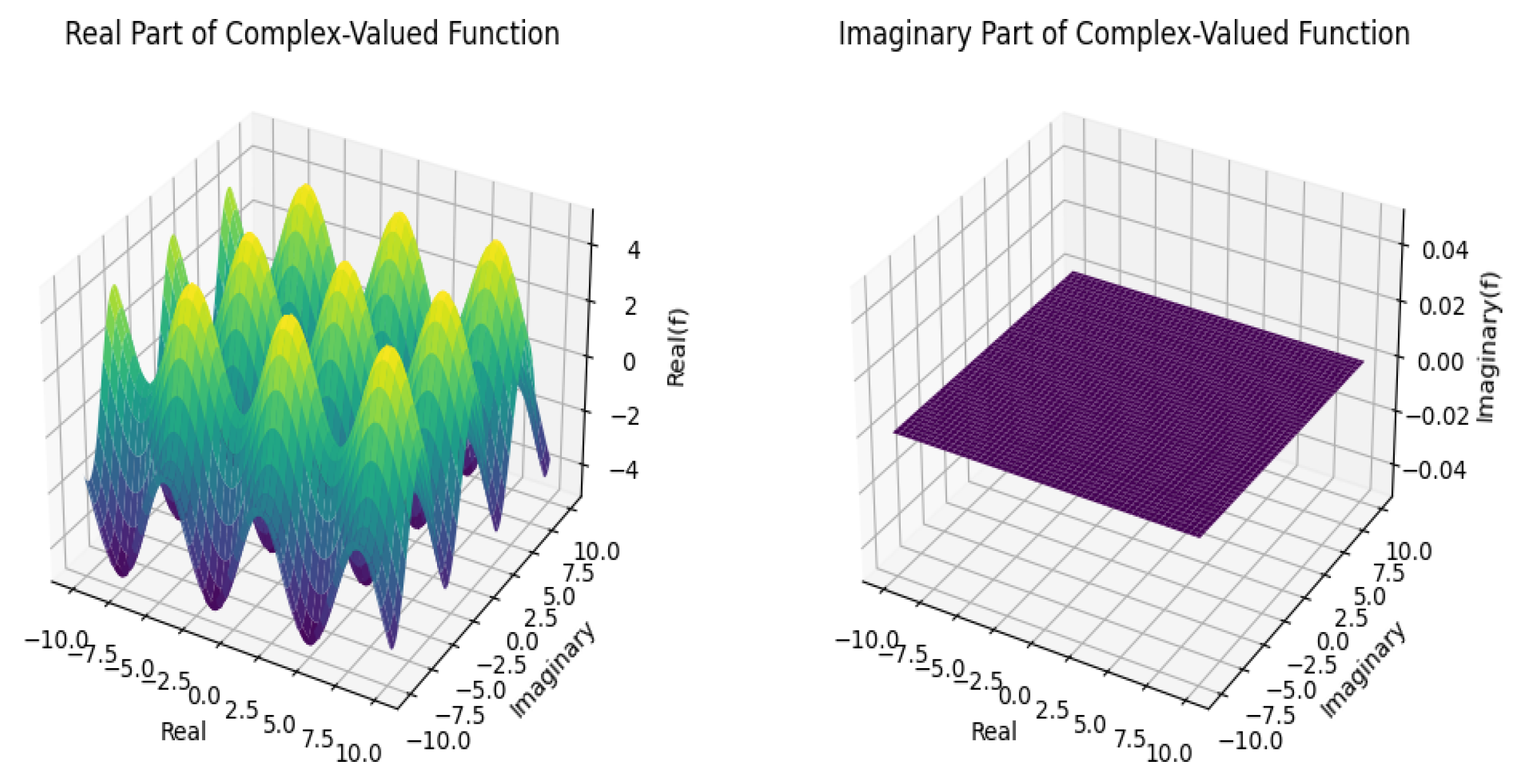
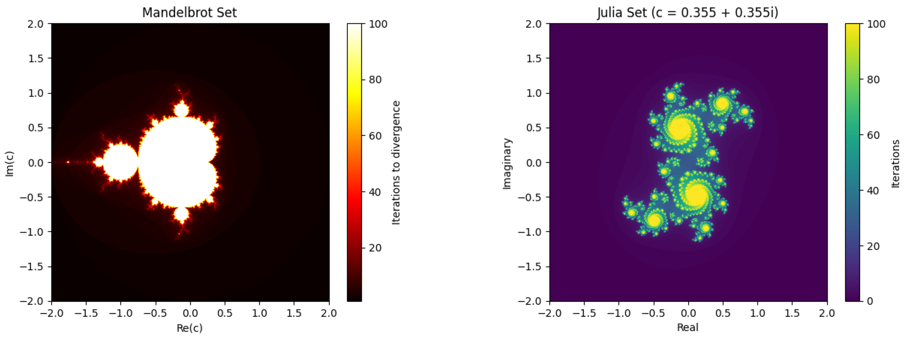
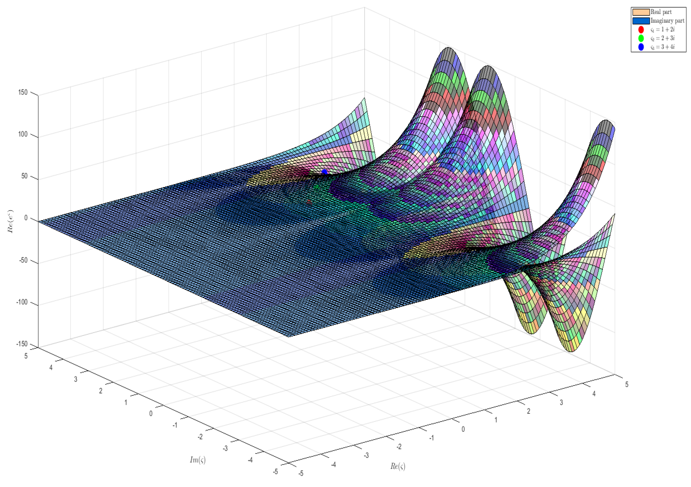
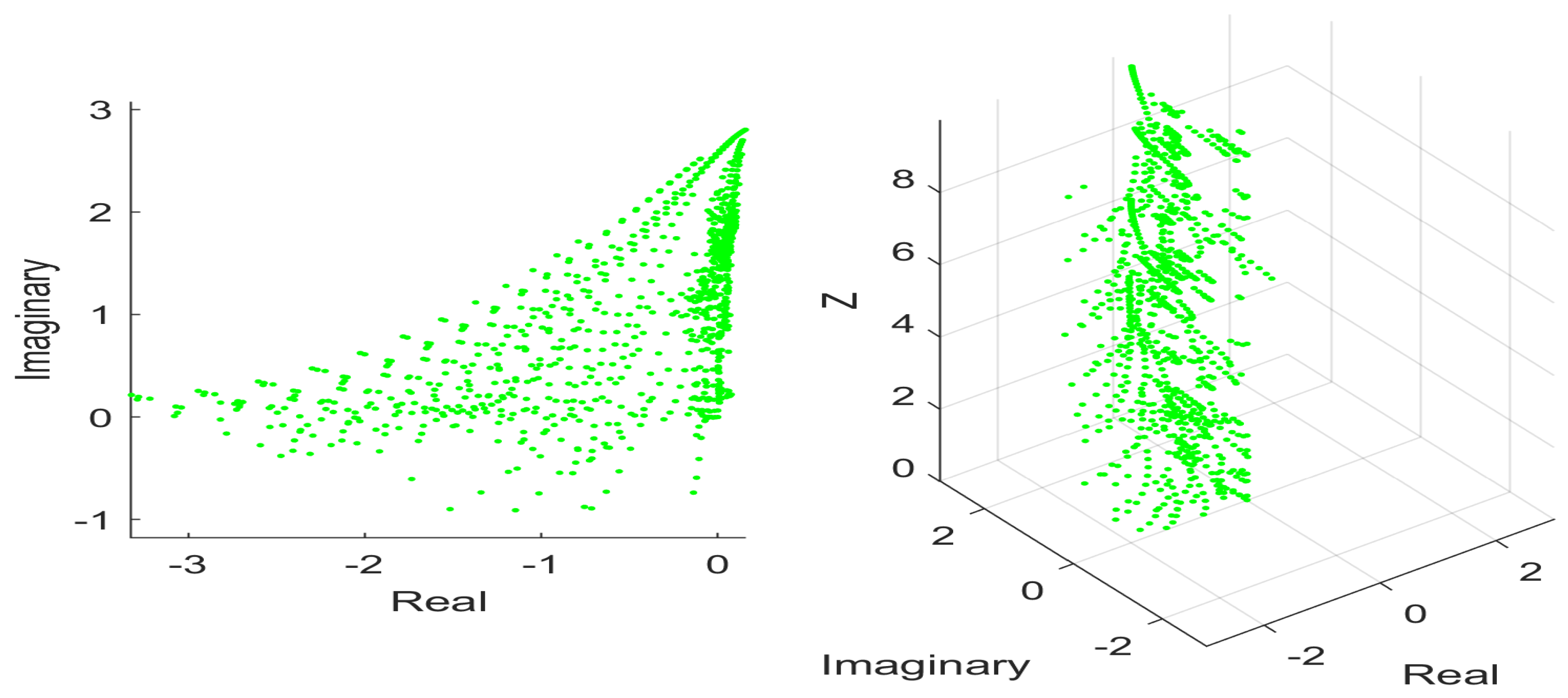
Creating a Connection between Fractals, Fixed-Point, and Complex-Valued Functions

A profound relation between fixed points and fractals can be seen in the nonlinear sciences.   $z_{n+1}=z_n^2+c$ is utilized to establish the Mandelbrot set. Here, c represents a constant complex number and $z_n$ represents a complex value that indicates the current iteration’s progress. Now, let us see how a fixed point acts. Assume that we select $c=0$ according to the Mandelbrot formula. Initially, the series $z_0,z_1,z_2,\dots$ will perpetually begin at zero and end at that point. For this reason, $z_{n+1}=z_n^2+0=z_n^2$; as a result, $z_n$ is a constant. A single point at the origin, which represents the fixed point, is visible when we display the Mandelbrot set under this scenario.

The Figure 3 representations of the Mandelbrot Set and Julia set, where each point in the complex plane corresponds to a pixel on the image. The color of each pixel indicates the number of iterations required for the corresponding complex number to diverge under the iterative process defined by the Mandelbrot/Julia equation. Let us investigate a fractal pattern now. There are numerous beginning values of $z_0$ for which the sequence of $z_n$ may diverge to infinity if we select c so that it is beyond the Mandelbrot set (e.g., $c=1$). The complex fractal structure that makes the Mandelbrot set famous is visible when the set is plotted for this particular situation. The border of the set separates areas where the sequence differs (outside the set) from areas where it stays bounded (inside the set), creating intricate and infinitely precise boundaries that are self-similar at different sizes.

Figure 3. Fractals of Mandelbrot set and Julia set.

In conclusion, the Mandelbrot set provides an enthralling example of the interaction between mathematical ideas and aesthetic beauty by illuminating how fixed points (like at $c=0$) and fractal patterns (like the complex set boundary) have a close relationship employing iterative operations in complex-valued spaces.

Furthermore, the Julia set sheds additional light on the connection underlying fixed points as well as fractals with complex structures and is closely related to the Mandelbrot set. A particular equation $z_{n+1}=z_n^2+c$ defines the Mandelbrot set, whereas the Julia set is concerned with the behavior of the loops of an individual complex value within the identical iterative technique.

Choose a point c on the complex plane to see if you can make this link. For each c, we can generate a corresponding Julia set by iteratively applying the function $f(z)=z^2+c$ to various initial values of $z_0$. The Julia set consists of all points in the complex plane for which the iterates of $z_0$ under $f(z)$ remain bounded.

Now, here is where the connection to the Mandelbrot set arises: every point in the Mandelbrot set corresponds to a parameter c for which the corresponding Julia set is connected (i.e., not fragmented). Conversely, points outside the Mandelbrot set correspond to values of c for which the corresponding Julia set is fragmented, exhibiting intricate fractal patterns.

Thus, by exploring the Julia sets associated with different values of c, we gain further insight into the dynamics of the Mandelbrot set. The boundary of the Mandelbrot set precisely delineates the regions in the complex plane where the associated Julia sets transition between connected and fragmented forms, showcasing the delicate interplay between fixed points and fractals in complex dynamics. Through the lens of the Julia set, we witness how the presence or absence of fixed points influences the formation of fractal structures, offering a deeper understanding of the underlying principles governing complex dynamical systems.

2. Complex-Valued Suprametric Spaces and Related Fixed Point Results

Let $\mathbb{C}$ be the set of complex numbers, and let $a_1,a_2\in \mathbb{C}$. We define a partial order ≾ on $\mathbb{C}$ as follows:

For any $a_1,a_2\in \mathbb{C}$, we say $a_1\precsim a_2$ if any of the following conditions hold:

• $Re(a_1)=Re(a_2)$ and $Im(a_1)<Im(a_2)$;
• $Re(a_1)<Re(a_2)$ and $Im(a_1)=Im(a_2)$;
• $Re(a_1)<Re(a_2)$ and $Im(a_1)<Im(a_2)$;
• $Re(a_1)=Re(a_2)$ and $Im(a_1)=Im(a_2)$.

In other words, $a_1$ is less than or equal to $a_2$ if either $a_1$ and $a_2$ have the same real part and $a_1$ has a smaller imaginary part, if  $a_1$ has a smaller real part regardless of the imaginary parts, if both real and imaginary parts of $a_1$ are smaller than those of $a_2$, or if $a_1$ and $a_2$ are identical.

Definition 1.

Let $\mathcal{M}$ be a set, and let ${\mathcal{S}}_d$ be a function from $\mathcal{M}\times \mathcal{M}$ to the set of complex numbers $\mathbb{C}$. Define a partial order ≾ on $\mathcal{M}$ as follows:

For any $\theta ,\eta \in \mathcal{M}$:

$$\theta \precsim \eta$$

if and only if ${\mathcal{S}}_d(\theta ,\eta )$ is a non-negative real number.

With this partial order, we can define a complex-valued suprametric space as follows:

• Non-negativity: For any $\theta ,\eta \in \mathcal{M}$, ${\mathcal{S}}_d(\theta ,\eta )$ is a non-negative real number if and only if $\theta \precsim \eta$.
• Identity of Indiscernible: For any $\theta ,\eta \in \mathcal{M}$, ${\mathcal{S}}_d(\theta ,\eta )=0$ if and only if $\theta =\eta$.
• Conjugate Symmetry: For any $\theta ,\eta \in \mathcal{M}$, ${\mathcal{S}}_d(\theta ,\eta )=\overline{{\mathcal{S}}_d(\eta ,\theta )}$ if and only if $\theta \precsim \eta$ and $\eta \precsim \theta$.
• Supratriangle Inequality: For any $\theta ,\eta ,\vartheta \in \mathcal{M}$ and some constant $\rho \in {\mathbb{R}}^{+}$, we have

  $${\mathcal{S}}_d(\theta ,\vartheta )\le {\mathcal{S}}_d(\theta ,\eta )+{\mathcal{S}}_d(\eta ,\vartheta )+\rho ·{\mathcal{S}}_d(\theta ,\eta )·{\mathcal{S}}_d(\eta ,\vartheta )$$
  if and only if $\theta \precsim \eta$ and $\eta \precsim \vartheta$.

Then, ${\mathcal{S}}_d$ is called a complex-valued suprametric on $\mathcal{M}$, and  $(\mathcal{M},{\mathcal{S}}_d)$ is called a complex-valued suprametric space ( ${\mathcal{C}}_s$-space). This definition provides a way to characterize a ${\mathcal{C}}_s$-space using a partial order on the elements of the space, based on the non-negativity of the suprametric function.

The aforementioned ${\mathcal{C}}_s$-space encompasses suprametric space [2], complex-valued metric space [3], and some additional spaces (refer to [4,5,6] for more details). In the year 1922, Polish mathematician Stefan Banach published the contraction mapping theorem, which launched the metric fixed point hypothesis, one of the most rapidly developing fields of research in the past century. It is constructed simultaneously as a theoretical concept and as a method for addressing problems across various conceptual and specific fields, including circuit models [7], integral and differential algorithms and inclusions [8,9,10,11,12,13], complex systems [14], and others [15].

Example 1.

Consider the set $\mathcal{M}=\mathbb{C}$(the set of complex numbers). Define the function ${\mathcal{S}}_d:\mathcal{M}\times \mathcal{M}\to \mathbb{C}$ as follows:

$${\mathcal{S}}_d({\varsigma }_1,{\varsigma }_2)=\frac{1}{2}|e^{{\varsigma }_1}-e^{{\varsigma }_2}|;$$

where $e^p$ denotes the exponential function applied to the complex number p, and  ${\varsigma }_1,{\varsigma }_2\in \mathbb{C}$. Let us define the partial order ≾ on $\mathcal{M}$ as follows: For any ${\varsigma }_1,{\varsigma }_2\in \mathbb{C}$, we say ${\varsigma }_1\precsim {\varsigma }_2\iff \frac{1}{2}|e^{{\varsigma }_1}-e^{{\varsigma }_2}|$ is an non-negative real number.

Now, let ${\varsigma }_1=1+2i$; ${\varsigma }_2=2+3i$; ${\varsigma }_3=3+4i$. We will choose $\rho =1$ for simplicity.

We have ${\mathcal{S}}_d({\varsigma }_1,{\varsigma }_2)=\frac{1}{2}|e^{{\varsigma }_1}-e^{{\varsigma }_2}|$; ${\mathcal{S}}_d({\varsigma }_2,{\varsigma }_3)=\frac{1}{2}|e^{{\varsigma }_2}-e^{{\varsigma }_3}|$; ${\mathcal{S}}_d({\varsigma }_1,{\varsigma }_3)=\frac{1}{2}|e^{{\varsigma }_1}-e^{{\varsigma }_3}|$.

Now, we have

$$e^{{\varsigma }_1}=e^{1+2i}\approx -1.1312+2.4717i;$$

$$e^{{\varsigma }_2}=e^{2+3i}\approx -7.3151+1.0427i;$$

$$e^{{\varsigma }_3}=e^{3+4i}\approx -13.1288-15.2008i.$$

One can easily verify non-negativity and the identity of indiscernible and conjugate symmetry conditions of Definition 1.

Now, we will check supratriangle inequality. $|{\mathcal{S}}_d({\varsigma }_1,{\varsigma }_3)|=\frac{1}{2}|e^{{\varsigma }_1}-e^{{\varsigma }_3}|\approx 10.6801$.

$$\begin{array}{cc}\hfill & |{\mathcal{S}}_d({\varsigma }_1,{\varsigma }_2)|+|{\mathcal{S}}_d({\varsigma }_2,{\varsigma }_3)|+\rho .|{\mathcal{S}}_d({\varsigma }_1,{\varsigma }_2)||{\mathcal{S}}_d({\varsigma }_2,{\varsigma }_3)|\hfill \\ \hfill & =\frac{1}{2}|e^{{\varsigma }_1}-e^{{\varsigma }_2}|+\frac{1}{2}|e^{{\varsigma }_2}-e^{{\varsigma }_3}|+\frac{1}{4}|e^{{\varsigma }_1}-e^{{\varsigma }_2}||e^{{\varsigma }_2}-e^{{\varsigma }_3}|\hfill \\ \hfill & \approx 39.1746.\hfill \end{array}$$

Thus, $|{\mathcal{S}}_d({\varsigma }_1,{\varsigma }_3)|\le |{\mathcal{S}}_d({\varsigma }_1,{\varsigma }_2)|+|{\mathcal{S}}_d({\varsigma }_2,{\varsigma }_3)|+\rho .|{\mathcal{S}}_d({\varsigma }_1,{\varsigma }_2)||{\mathcal{S}}_d({\varsigma }_2,{\varsigma }_3)|$.

Hence, $(\mathcal{M},d)$ is a ${\mathcal{C}}_s$-space.

The Figure 4 visualizes the exponential function $e^{\varsigma }$ over a grid of complex numbers, displaying both real and imaginary parts. It includes marked points for the complex numbers $1+2i$, $2+3i$, and  $3+4i$ with respective exponential values plotted. The graph effectively shows the real part of the exponential function on the z-axis, helping to understand the complex exponential transformation.

Figure 4. Three-Dimensional Plot of Complex Exponential Function $e^p$.

Similarity Assessment of Linguistic Terms Using Complex-Valued Suprametric Approach

Example 2.

Let us represent the linguistic terms “cold”, “warm”, and “hot” by the complex numbers as follows:

$$\begin{array}{cc}\hfill “\mathrm{cold}”& \mathrm{is}\mathrm{represented}\mathrm{by}{𝕢}_1=-2+3i;\hfill \\ \hfill “\mathrm{warm}”& \mathrm{is}\mathrm{represented}\mathrm{by}{𝕢}_2=1+2i;\hfill \\ \hfill “\mathrm{hot}”& \mathrm{is}\mathrm{represented}\mathrm{by}{𝕢}_3=3-i.\hfill \end{array}$$

We define a fuzzy relation ${\mathcal{F}}_r$ between these linguistic terms as follows:

$${\mathcal{F}}_r=\left[\begin{array}{ccc}1& 0.8& 0.3\\ 0.8& 1& 0.6\\ 0.3& 0.6& 1\end{array}\right].$$

Here, the entry ${\mathcal{F}}_r(i,j)$ represents the degree of membership of linguistic term ${𝕢}_i$ in relation to ${𝕢}_j$, indicating how strongly ${𝕢}_i$ is related to ${𝕢}_j$.

We will apply the concept of a ${\mathcal{C}}_s$-space to analyze this fuzzy relation.

Let us analyze the fuzzy relation ${\mathcal{F}}_r$ using the properties of a ${\mathcal{C}}_s$-space:

• Non-negativity: For any ${𝕢}_i,{𝕢}_j\in \{{𝕢}_1,{𝕢}_2,{𝕢}_3\}$, ${\mathcal{F}}_r(i,j)$ is a non-negative real number if and only if ${𝕢}_i\precsim {𝕢}_j$.
• Identity of Indiscernibles: For any ${𝕢}_i,{𝕢}_j\in \{{𝕢}_1,{𝕢}_2,{𝕢}_3\}$, ${\mathcal{F}}_r(i,j)=0$ if and only if ${𝕢}_i={𝕢}_j$.
• Conjugate Symmetry: For any ${𝕢}_i,{𝕢}_j\in \{{𝕢}_1,{𝕢}_2,{𝕢}_3\}$, ${\mathcal{F}}_r(i,j)=\overline{{\mathcal{F}}_r(j,i)}$ if and only if ${𝕢}_i\precsim {𝕢}_j$ and ${𝕢}_j\precsim {𝕢}_i$.
• Supratriangle Inequality: For any ${𝕢}_i,{𝕢}_j,{𝕢}_k\in \{{𝕢}_1,{𝕢}_2,{𝕢}_3\}$ and some constant $\rho \in {\mathbb{R}}^{+}$, we have

  $${\mathcal{F}}_r(i,k)\le {\mathcal{F}}_r(i,j)+{\mathcal{F}}_r(j,k)+\rho ·{\mathcal{F}}_r(i,j)·{\mathcal{F}}_r(j,k)$$

  if and only if ${𝕢}_i\precsim {𝕢}_j$ and ${𝕢}_j\precsim {𝕢}_k$.

Let us check if these properties hold for the given fuzzy relation ${\mathcal{F}}_r$:

• Non-negativity:

  •

  ${\mathcal{F}}_r(1,2)=0.8$, which means ${𝕢}_1\precsim {𝕢}_2$;

  •

  ${\mathcal{F}}_r(2,3)=0.6$, which means ${𝕢}_2\precsim {𝕢}_3$;

  •

  All other values are also non-negative, indicating the non-negativity property.

• Identity of Indiscernibles:

  •

  ${\mathcal{F}}_r(1,1)=1$, indicating ${𝕢}_1={𝕢}_1$;

  •

  ${\mathcal{F}}_r(2,2)=1$, indicating ${𝕢}_2={𝕢}_2$;

  •

  ${\mathcal{F}}_r(3,3)=1$, indicating ${𝕢}_3={𝕢}_3$.

• Conjugate Symmetry:

  •

  ${\mathcal{F}}_r(1,2)=0.8$ and ${\mathcal{F}}_r(2,1)=0.8$, indicating ${𝕢}_1\precsim {𝕢}_2$ and ${𝕢}_2\precsim {𝕢}_1$;

  •

  ${\mathcal{F}}_r(1,3)=0.3$ and ${\mathcal{F}}_r(3,1)=0.3$, indicating ${𝕢}_1\precsim {𝕢}_3$ and ${𝕢}_3\precsim {𝕢}_1$;

  •

  ${\mathcal{F}}_r(2,3)=0.6$ and ${\mathcal{F}}_r(3,2)=0.6$, indicating ${𝕢}_2\precsim {𝕢}_3$ and ${𝕢}_3\precsim {𝕢}_2$.

• Supratriangle Inequality:

  •

  For ${𝕢}_1=-2+3i$, ${𝕢}_2=1+2i$, and  ${𝕢}_3=3-i$:

  $$\begin{array}{cc}\hfill {\mathcal{F}}_r(1,3)& \le {\mathcal{F}}_r(1,2)+{\mathcal{F}}_r(2,3)+\rho ·{\mathcal{F}}_r(1,2)·{\mathcal{F}}_r(2,3)\hfill \\ \hfill 0.3& \le 0.8+0.6+\rho ·0.8·0.6\hfill \\ \hfill 0.3& \le 0.8+0.6+0.48\rho \hfill \\ \hfill 0.3-0.3& \le 1.4+0.48\rho -0.3\hfill \\ \hfill 0& \le 1.4+0.48\rho \hfill \\ \hfill -1.4& \le 0.48\rho \hfill \\ \hfill \frac{-1.4}{0.48}& \le \rho \hfill \\ \hfill \frac{-35}{12}& \le \rho .\hfill \end{array}$$

  Since $\rho$ is a positive constant, $\frac{-35}{12}$ satisfies the supratriangle inequality.

The characteristics of a ${\mathcal{C}}_s$-space are satisfied by the fuzzy-relation ${\mathcal{F}}_r$ constructed on the language terms “cold”, “warm”, and “hot”. This analysis illustrates the use of ${\mathcal{C}}_s$-spaces in fuzzy logic by providing a pertinent similarity measure between linguistic concepts in a fuzzy logic system.

This idea of ${\mathcal{C}}_s$-space can be extended to the field of fuzzy logic. Now, we create a method to assess how similar two fuzzy sets that are encoded through complex-valued feature vectors are to one another.

Suppose a dataset is made up of complex-valued feature vectors that represent fuzzy sets. In order to differentiate between those sets of fuzzy data according to their distinctive characteristic vectors, we wish to create a similarity metric.

Example 3.

Let us consider a dataset containing three fuzzy sets represented by complex-valued feature vectors:

$${\mathbf{A}}_1=(1+2i,3-4i,5+i),{\mathbf{A}}_2=(2-3i,1+2i,4-5i),{\mathbf{A}}_3=(3-i,2+3i,6-2i).$$

To compare these feature vectors and evaluate the degree of similarity between the fuzzy sets, we will create an independent complex-valued suprametric similarity measure.

Based on the provided fuzzy sets, let us construct an appropriate complex-valued suprametric similarity measure. We will apply the following definition:

$${\mathcal{S}}_d({\mathbf{A}}_i,{\mathbf{A}}_j)=\left|{\displaystyle \sum _{k=1}^3}\frac{{\mathbf{A}}_i(k)}{\parallel {\mathbf{A}}_i\parallel }·\frac{{\mathbf{A}}_j(k)}{\parallel {\mathbf{A}}_j\parallel }\right|,$$

where $\parallel \mathbf{A}\parallel$ depicts the Euclidean norm of vector $\mathbf{A}$, and  $\mathbf{A}(k)$ specifies that k-th element of vector $\mathbf{A}$.

Now, we will use the proposed complex-valued suprametric similarity measure to calculate the similarity among each pair of fuzzy sets:

• For fuzzy sets ${\mathbf{A}}_1$ and ${\mathbf{A}}_2$:

  $$\begin{array}{cc}\hfill {\mathcal{S}}_d({\mathbf{A}}_1,{\mathbf{A}}_2)& =\left|\frac{(1+2i)(2-3i)}{\sqrt{(1+2i)(1-2i)}·\sqrt{(2-3i)(2+3i)}}\right.\hfill \\ \hfill & +\frac{(3-4i)(1+2i)}{\sqrt{(3-4i)(3+4i)}·\sqrt{(1+2i)(1-2i)}}\hfill \\ \hfill & +\left.\frac{(5+i)(4-5i)}{\sqrt{(5+i)(5-i)}·\sqrt{(4-5i)(4+5i)}}\right|\hfill \\ \hfill & =\left|\frac{(2-3i)-8i+20-21i}{\sqrt{5+5i}·\sqrt{13}}\right|\hfill \\ \hfill & =\left|\frac{22-25i}{\sqrt{5+5i}·\sqrt{13}}\right|\hfill \\ \hfill & \approx 0.2797.\hfill \end{array}$$
• For fuzzy sets ${\mathbf{A}}_1$ and ${\mathbf{A}}_3$:

  $$\begin{array}{cc}\hfill {\mathcal{S}}_d({\mathbf{A}}_1,{\mathbf{A}}_3)& =\left|\frac{(1+2i)(3-i)}{\sqrt{(1+2i)(1-2i)}·\sqrt{(3-i)(3+i)}}\right.\hfill \\ \hfill & +\frac{(3-4i)(2+3i)}{\sqrt{(3-4i)(3+4i)}·\sqrt{(2+3i)(2-3i)}}\hfill \\ \hfill & +\left.\frac{(5+i)(6-2i)}{\sqrt{(5+i)(5-i)}·\sqrt{(6-2i)(6+2i)}}\right|\hfill \\ \hfill & =\left|\frac{5-3i+15i-2}{\sqrt{5+5i}·\sqrt{13}}\right|\hfill \\ \hfill & =\left|\frac{3+12i}{\sqrt{5+5i}·\sqrt{13}}\right|\hfill \\ \hfill & \approx 0.8543.\hfill \end{array}$$
• For fuzzy sets ${\mathbf{A}}_2$ and ${\mathbf{A}}_3$:

  $$\begin{array}{cc}\hfill {\mathcal{S}}_d({\mathbf{A}}_2,{\mathbf{A}}_3)& =\left|\frac{(2-3i)(3-i)}{\sqrt{(2-3i)(2+3i)}·\sqrt{(3-i)(3+i)}}\right.\hfill \\ \hfill & +\frac{(1+2i)(2+3i)}{\sqrt{(1+2i)(1-2i)}·\sqrt{(2+3i)(2-3i)}}\hfill \\ \hfill & +\left.\frac{(4-5i)(6-2i)}{\sqrt{(4-5i)(4+5i)}·\sqrt{(6-2i)(6+2i)}}\right|\hfill \\ \hfill & =\left|\frac{9-i-6-2i}{\sqrt{13}·\sqrt{13}}\right|\hfill \\ \hfill & =\left|\frac{3-3i}{13}\right|\hfill \\ \hfill & \approx 0.2308.\hfill \end{array}$$

A quantitative assessment of the connections among the sets of fuzzy data in the provided ${\mathcal{C}}_s$-space is provided by the computed similarity values. To efficiently evaluate the similarity among fuzzy sets, those metrics of similarity can be applied in fuzzy reasoning operations like fuzzy detection of patterns or fuzzy set classification.

Example 4.

Suppose we have a dataset with n fuzzy sets that are expressed by complex-valued characteristic vectors. Through the use of ${\mathcal{C}}_s$-space, we hope to cluster such fuzzy sets under k clusters according to their resemblance.

The following are given:

•

n fuzzy sets $\{{\mathbf{A}}_1,{\mathbf{A}}_2,\dots ,{\mathbf{A}}_n\}$, each represented by a complex-valued feature vector in ${\mathbb{C}}^m$;

•

k initial cluster centers $\{C_1,C_2,\dots ,C_k\}$, where each $C_i$ is also a complex-valued feature vector in ${\mathbb{C}}^m$.

Let us define the complex-valued suprametric similarity measure ${\mathcal{S}}_d$ between two complex-valued feature vectors $\mathbf{X}$ and $\mathbf{Y}$ as:

$${\mathcal{S}}_d(\mathbf{X},\mathbf{Y})=\left|{\displaystyle \sum _{i=1}^m}\frac{\mathbf{X}(i)}{\parallel \mathbf{X}\parallel }·\frac{\mathbf{Y}(i)}{\parallel \mathbf{Y}\parallel }\right|,$$

where

•

$\mathbf{X}(i)$ and $\mathbf{Y}(i)$ denote the i-th elements of vectors $\mathbf{X}$ and $\mathbf{Y}$, respectively;

•

$\parallel \mathbf{X}\parallel$ and $\parallel \mathbf{Y}\parallel$ represent the Euclidean norms of vectors $\mathbf{X}$ and $\mathbf{Y}$, respectively.

Let us demonstrate the application of the above solution approach to a specific example with three fuzzy sets represented by complex-valued feature vectors.

Consider the following three fuzzy sets:

$${\mathbf{A}}_1=(1+2i,3-4i,5+i),$$

$${\mathbf{A}}_2=(2-3i,1+2i,4-5i),$$

$${\mathbf{A}}_3=(3-i,2+3i,6-2i).$$

Now, we will demonstrate and perform the following steps outlined in the solution approach to cluster these fuzzy sets into two clusters.

• Step 1: Initialization

We randomly initialize two cluster centers:

$$C_1={\mathbf{A}}_1=(1+2i,3-4i,5+i),$$

$$C_2={\mathbf{A}}_2=(2-3i,1+2i,4-5i).$$

• Step 2: Assigning

For each fuzzy set ${\mathbf{A}}_i$, we calculate its similarity to each cluster center:

• For ${\mathbf{A}}_1$:

  $${\mathcal{S}}_d({\mathbf{A}}_1,C_1)\approx 1(\mathrm{since}{\mathbf{A}}_1\mathrm{is}\mathrm{identical}\mathrm{to}{C}_1),$$

  $${\mathcal{S}}_d({\mathbf{A}}_1,C_2)\approx 0.2797.$$
• For ${\mathbf{A}}_2$:

  $${\mathcal{S}}_d({\mathbf{A}}_2,C_1)\approx 0.2797,$$

  $${\mathcal{S}}_d({\mathbf{A}}_2,C_2)\approx 1(\mathrm{since}{\mathbf{A}}_2\mathrm{is}\mathrm{identical}\mathrm{to}{C}_2).$$
• For ${\mathbf{A}}_3$:

  $${\mathcal{S}}_d({\mathbf{A}}_3,C_1)\approx 0.8543,$$

  $${\mathcal{S}}_d({\mathbf{A}}_3,C_2)\approx 0.2308.$$

• Step 3: Update

We update the cluster centers based on the assigned fuzzy sets:

$$C_1=\frac{{\mathbf{A}}_1+{\mathbf{A}}_3}{2}=\left(\frac{1+2i+3-i}{2},\frac{3-4i+2+3i}{2},\frac{5+i+6-2i}{2}\right)=(2+0.5i,2+0.5i,5-0.5i),$$

$$C_2={\mathbf{A}}_2=(2-3i,1+2i,4-5i).$$

• Step 4: Convergence

We repeat steps 2 and 3 until convergence. In this case, the assignment does not change after the first iteration, indicating convergence.

Therefore, the final clustering is as follows:

•

Cluster 1: $\{{\mathbf{A}}_1,{\mathbf{A}}_3\}$;

•

Cluster 2: $\{{\mathbf{A}}_2\}$.

This completes the proof of concept for fuzzy clustering using the complex-valued suprametric similarity measure.

The presented Algorithm 1, leveraging complex-valued suprametric similarity, offers a novel approach to clustering fuzzy sets represented by complex-valued feature vectors. Unlike traditional clustering methods, this algorithm incorporates the intricate relationships captured by complex numbers, providing a nuanced measure of similarity that can accommodate both magnitude and phase differences in data. This technique is particularly well-suited for applications in soft computing, where the inherent fuzziness and complexity of data can be better managed using complex-valued metrics. By iteratively refining cluster centers based on the unique suprametric properties, the algorithm ensures robust and meaningful clustering outcomes. In the realm of complex-valued metric spaces endowed with partial orders, a fascinating interplay between geometric structure and order relationships unfolds.

Algorithm 1 Fuzzy Clustering Using Complex-Valued Suprametric Similarity

1: Input: Dataset of n fuzzy sets represented by complex-valued feature vectors, k initial cluster centers 2: Output: Cluster assignments 3: procedure Fuzzy Clustering ( $\{{\mathbf{A}}_1,{\mathbf{A}}_2,\dots ,{\mathbf{A}}_n\},\{C_1,C_2,\dots ,C_k\}$) 4:      Step 1: Initialization 5:      Initialize k cluster centers $\{C_1,C_2,\dots ,C_k\}$ randomly 6:      7:      Step 2: Assigning 8:      repeat 9:            for  $i=1$ to n do 10:                for  $j=1$ to k do 11:                     Compute ${\mathcal{S}}_d({\mathbf{A}}_i,C_j)$ using the complex-valued suprametric similarity measure 12:                end for 13:                Assign ${\mathbf{A}}_i$ to the cluster with the highest similarity 14:           end for 15:          16:           Step 3: Update 17:           for  $j=1$ to k do 18:                Update cluster center $C_j$ as the mean of all fuzzy sets assigned to cluster j 19:           end for 20:     until No change in cluster assignments 21:       22:     Output: Cluster assignments 23: end procedure

Definition 2.

Let $\mathcal{M}$ be the set of ${\mathcal{C}}_s$-space with partial order ≾, and also suppose a subset $\mathcal{A}\subseteq \mathcal{M}$. An element θ of $\mathcal{A}$ is said to be an interior point of $\mathcal{A}$ if there exists a positive real number r such that the ϵ-ball centered at θ with radius r, denoted as ${\mathcal{B}}_{ϵ}(\theta ,r)$, is entirely contained within $\mathcal{A}$.

Formally, θ is an interior point of $\mathcal{A}$ if there exists $r>0$ such that the ϵ-ball ${\mathcal{B}}_{ϵ}(\theta ,r)=\{\eta \in \mathcal{M}:{\mathcal{S}}_d(\theta ,\eta )<r\}$ is a subset of $\mathcal{A}$.

In simpler terms, an interior point of $\mathcal{A}$ is a point within $\mathcal{A}$ for which there exists a small enough ϵ-ball centered at that point such that all points within that ϵ-ball also belong to $\mathcal{A}$.

A point $\theta \in \mathcal{M}$ is called a limit point of $\mathcal{A}$ whenever for every $0\prec r\in \mathbb{C}$,

$$\mathcal{B}(\theta ,r)\cap (\mathcal{A}\setminus \mathcal{M})\ne \varnothing .$$

Definition 3.

A subset $\mathcal{A}$ of a ${\mathcal{C}}_s$-space $(\mathcal{M},{\mathcal{S}}_d)$ is considered closed if it contains all its limit points. Formally, $\mathcal{A}$ is closed if every limit point of $\mathcal{A}$ is also contained in $\mathcal{A}$—that is, for every limit point x of $\mathcal{A}$, $\theta \in \mathcal{A}$.

Definition 4.

A subset U of a ${\mathcal{C}}_s$-space $(\mathcal{M},{\mathcal{S}}_d)$ is considered open if, for every point x in U, there exists a positive real number ϵ such that the ϵ-ball ${\mathcal{B}}_{ϵ}(\theta )$ is entirely contained in U. Formally, U is open if for every $\theta \in U$, there exists $ϵ>0$ such that ${\mathcal{B}}_{ϵ}(\theta )\subseteq U$, where ${\mathcal{B}}_{ϵ}(\theta )=\{\eta \in \mathcal{M}:{\mathcal{S}}_d(\theta ,\eta )<ϵ\}$.

Proposition 1.

Let $(\mathcal{M},{\mathcal{S}}_d)$ be a ${\mathcal{C}}_s$-space, then each open ball is an open set.

Proposition 2.

τ defines a topology on ${\mathcal{C}}_s$-space $(\mathcal{M},{\mathcal{S}}_d)$ and the family of open balls forms a base of the topology τ.

Proposition 3.

The topology τ is Hausdorff.

Proposition 4.

Let $(\mathcal{M},{\mathcal{S}}_d)$ be a ${\mathcal{C}}_s$-space. If a sequence ${\{{\theta }_n\}}_{n\in \mathbb{N}}\subset \mathcal{M}$ has a limit, then it is unique.

Definition 5.

Let $(\mathcal{M},{\mathcal{S}}_d)$ be a ${\mathcal{C}}_s$-space. If for every $c\in \mathbb{C}$ with $0\prec c$ there is $n_0\in \mathbb{N}$ such that for all $n>n_0,{\mathcal{S}}_d({\theta }_n,{\theta }_{n+m})\prec c$, then $\{{\theta }_n\}$ is called a Cauchy sequence in $(\mathcal{M},{\mathcal{S}}_d)$.

Definition 6.

If every Cauchy sequence is convergent in a ${\mathcal{C}}_s$-space $(\mathcal{M},{\mathcal{S}}_d)$, then $(\mathcal{M},{\mathcal{S}}_d)$ is called a complete ${\mathcal{C}}_s$-space.

Definition 7.

Let $(\mathcal{M},{\mathcal{S}}_d)$ be a ${\mathcal{C}}_s$-space. If for every $c\in \mathbb{C}$ with $0\prec c$ there is $n_0\in \mathbb{N}$ such that for all $n>n_0,{\mathcal{S}}_d({\theta }_n,{\theta }_{n+m})\prec c$, then $\{{\theta }_n\}$ is called a Cauchy sequence in $(\mathcal{M},{\mathcal{S}}_d)$.

Definition 8.

If every Cauchy sequence is convergent in a ${\mathcal{C}}_s$-space $(\mathcal{M},{\mathcal{S}}_d)$. A mapping $\mathcal{O}:\mathcal{M}\to \mathcal{M}$ is said to be continuous at ϑ, if for every $0\prec ϵ$ there exists $0\prec \eta$ such that ${\mathcal{S}}_d(\mathcal{O}\theta ,\mathcal{O}\vartheta )\prec \eta$ whenever ${\mathcal{S}}_d(\theta ,\vartheta )\prec ϵ$. If  $\mathcal{O}$ is continuous at every point of $\mathcal{M}$ then it is said to be continuous.

Lemma 1.

Let $(\mathcal{M},{\mathcal{S}}_d)$ be a ${\mathcal{C}}_s$-space and let $\{{\theta }_n\}$ be a sequence in $\mathcal{M}$. Then, $\{{\theta }_n\}$ converges to x if and only if $|{\mathcal{S}}_d({\theta }_n,\theta )|\to 0$ as $n\to \infty$.

Lemma 2.

Let $(\mathcal{M},{\mathcal{S}}_d)$ be a ${\mathcal{C}}_s$-space and let $\{{\theta }_n\}$ be a sequence in $\mathcal{M}$. Then, $\{{\theta }_n\}$ is a Cauchy sequence iff $|{\mathcal{S}}_d({\theta }_n,{\theta }_{n+m})|\to 0$ as $n\to \infty$.

Theorem 1.

Let $(\mathcal{M},{\mathcal{S}}_d)$ be a complete ${\mathcal{C}}_s$-space. If  $\mathcal{H}$ and $\mathcal{O}$ are self mappings defined on $(\mathcal{M},{\mathcal{S}}_d)$ satisfying the below contraction:

$${\mathcal{S}}_d(\mathcal{H}\theta ,\mathcal{O}\eta )\precsim \wp .{\mathcal{S}}_d(\theta ,\eta )+\frac{\sigma {\mathcal{S}}_d(\theta ,\mathcal{H}\theta ){\mathcal{S}}_d(\eta ,\mathcal{O}\eta )+\upsilon {\mathcal{S}}_d(\eta ,\mathcal{H}\theta ){\mathcal{S}}_d(\theta ,\mathcal{O}\eta )}{1+{\mathcal{S}}_d(\theta ,\eta )},$$

for all $\theta ,\eta \in \mathcal{M}$, where $\wp ,\sigma ,\upsilon$ are non-negative real numbers with $\wp +\sigma +\upsilon <1$, then $\mathcal{H}$ and $\mathcal{O}$ have a unique common fixed point.

Proof. 

Let ${\theta }_0$ be an arbitrary point in $\mathcal{M}$ and define the sequence ${\theta }_{2k+1}=\mathcal{H}{\theta }_{2k},{\theta }_{2k+2}=\mathcal{O}{\theta }_{2k+1},k=0,1,2,\dots$

Then,

$$\begin{array}{cc}\hfill {\mathcal{S}}_d({\theta }_{2k+1},{\theta }_{2k+2})& ={\mathcal{S}}_d(\mathcal{H}{\theta }_{2k},\mathcal{O}{\theta }_{2k+1})\hfill \\ \hfill & \precsim \wp {\mathcal{S}}_d({\theta }_{2k},{\theta }_{2k+1})\hfill \\ \hfill & +\frac{\sigma {\mathcal{S}}_d({\theta }_{2k},\mathcal{H}{\theta }_{2k}){\mathcal{S}}_d({\theta }_{2k+1},\mathcal{O}{\theta }_{2k+1})+\upsilon {\mathcal{S}}_d({\theta }_{2k},\mathcal{O}{\theta }_{2k+1}){\mathcal{S}}_d({\theta }_{2k+1},\mathcal{H}{\theta }_{2k})}{1+{\mathcal{S}}_d({\theta }_{2k},{\theta }_{2k+1})}.\hfill \end{array}$$

Since ${\theta }_{2k+1}=\mathcal{H}{\theta }_{2k}$ implies ${\mathcal{S}}_d({\theta }_{2k+1},\mathcal{H}{\theta }_{2k})=0$, therefore

$${\mathcal{S}}_d({\theta }_{2k+1},{\theta }_{2k+2})\precsim \wp {\mathcal{S}}_d({\theta }_{2k},{\theta }_{2k+1})+\frac{\sigma {\mathcal{S}}_d({\theta }_{2k},{\theta }_{2k+1}){\mathcal{S}}_d({\theta }_{2k+1},{\theta }_{2k+2})}{1+{\mathcal{S}}_d({\theta }_{2k},{\theta }_{2k+1})},$$

so that

$$|{\mathcal{S}}_d({\theta }_{2k+1},{\theta }_{2k+2})|\le \wp |{\mathcal{S}}_d({\theta }_{2k},{\theta }_{2k+1})|+\frac{\sigma |{\mathcal{S}}_d({\theta }_{2k},{\theta }_{2k+1})||{\mathcal{S}}_d({\theta }_{2k+1},{\theta }_{2k+2})|}{|1+{\mathcal{S}}_d({\theta }_{2k},{\theta }_{2k+1})|}.$$

Since $|1+{\mathcal{S}}_d({\theta }_{2k},{\theta }_{2k+1})|>|{\mathcal{S}}_d({\theta }_{2k},{\theta }_{2k+1})|$, therefore $|{\mathcal{S}}_d({\theta }_{2k+1},{\theta }_{2k+2})|\le \wp |{\mathcal{S}}_d({\theta }_{2k},{\theta }_{2k+1})|+\sigma |{\mathcal{S}}_d({\theta }_{2k+1},{\theta }_{2k+2})|,$ so that

$$|{\mathcal{S}}_d({\theta }_{2k+1},{\theta }_{2k+2})|\le \frac{\wp }{1-\sigma }|{\mathcal{S}}_d({\theta }_{2k},{\theta }_{2k+1})|.$$

Also,

$$\begin{array}{cc}\hfill & {\mathcal{S}}_d({\theta }_{2k+2},{\theta }_{2k+3})\hfill \\ \hfill & ={\mathcal{S}}_d(\mathcal{O}{\theta }_{2k+1},\mathcal{H}{\theta }_{2k+2})\hfill \\ \hfill & ={\mathcal{S}}_d(\mathcal{H}{\theta }_{2k+2},\mathcal{O}{\theta }_{2k+1})\hfill \\ \hfill & \precsim \wp {\mathcal{S}}_d({\theta }_{2k+2},{\theta }_{2k+1})\hfill \\ \hfill & +\frac{\sigma {\mathcal{S}}_d({\theta }_{2k+2},\mathcal{H}{\theta }_{2k+2}){\mathcal{S}}_d({\theta }_{2k+1},\mathcal{O}{\theta }_{2k+1})+\upsilon {\mathcal{S}}_d({\theta }_{2k+1},\mathcal{H}{\theta }_{2k+2}){\mathcal{S}}_d({\theta }_{2k+2},\mathcal{O}{\theta }_{2k+1})}{1+{\mathcal{S}}_d({\theta }_{2k+2},{\theta }_{2k+1})},\hfill \end{array}$$

so that

$$|{\mathcal{S}}_d({\theta }_{2k+2},{\theta }_{2k+3})|\le \wp |{\mathcal{S}}_d({\theta }_{2k+2},{\theta }_{2k+1})|+\frac{\sigma |{\mathcal{S}}_d({\theta }_{2k+2},{\theta }_{2k+3})||{\mathcal{S}}_d({\theta }_{2k+1},{\theta }_{2k+2})|}{|1+{\mathcal{S}}_d({\theta }_{2k+2},{\theta }_{2k+1})|}.$$

As $|1+{\mathcal{S}}_d({\theta }_{2k+2},{\theta }_{2k+1})|>|{\mathcal{S}}_d({\theta }_{2k+2},{\theta }_{2k+1})|$, therefore

$$|{\mathcal{S}}_d({\theta }_{2k+2},{\theta }_{2k+3})|\le \frac{\wp }{1-\sigma }|{\mathcal{S}}_d({\theta }_{2k+1},{\theta }_{2k+2})|.$$

By taking $c=\frac{\wp }{1-\sigma }$, then $|{\mathcal{S}}_d({\theta }_n,{\theta }_{n+1})|\le c|{\mathcal{S}}_d({\theta }_{n-1},{\theta }_n)|<|{\mathcal{S}}_d({\theta }_{n-1},{\theta }_n)|,\forall n$.

Thus, the sequence $\{{\mathcal{S}}_d({\theta }_n,{\theta }_{n+1})\}$ is decreasing and gratifies the following for all k,

$${\mathcal{S}}_d({\theta }_n,{\theta }_{n+1})\precsim c^{n-k}{\mathcal{S}}_d({\theta }_k,{\theta }_{k+1}),\mathrm{for}\mathrm{all}n>k.$$

$$|{\mathcal{S}}_d({\theta }_n,{\theta }_{n+1})|\le c^{n-k}|{\mathcal{S}}_d({\theta }_k,{\theta }_{k+1})|,\mathrm{for}\mathrm{all}n>k.$$

(1)

This implies that ${lim}_{n\to \infty }|{\mathcal{S}}_d({\theta }_n,{\theta }_{n+1})|\to 0$, thus there is $k\in \mathbb{N}$ in such a way that for every $n\ge k$; then, ${\mathcal{S}}_d({\theta }_n,\theta )\prec \delta$, where $0\prec \delta \in \mathbb{C}$.

Therefore,

$$|{\mathcal{S}}_d({\theta }_n,\theta )|<|\delta |=ϵ,\mathrm{for}\mathrm{all}n\ge k,\mathrm{where}\delta =\frac{ϵ}{\sqrt{2}}+i\frac{ϵ}{\sqrt{2}}.$$

(2)

Now, we shall prove that the sequence $\{{\theta }_n\}$ is Cauchy using Equations (1) and (2), supratriangle inequality, and for all $m,n$ in such a way that $n>m>k$; thus,

$${\mathcal{S}}_d({\theta }_m,{\theta }_n)\precsim {\mathcal{S}}_d({\theta }_m,{\theta }_{m+1})+{\mathcal{S}}_d({\theta }_{m+1},{\theta }_n)+\rho {\mathcal{S}}_d({\theta }_m,{\theta }_{m+1}){\mathcal{S}}_d({\theta }_{m+1},{\theta }_n).$$

$$\begin{array}{cc}\hfill |{\mathcal{S}}_d({\theta }_m,{\theta }_n)|& \le |{\mathcal{S}}_d({\theta }_m,{\theta }_{m+1})|+|{\mathcal{S}}_d({\theta }_{m+1},{\theta }_n)|+\rho |{\mathcal{S}}_d({\theta }_m,{\theta }_{m+1})||{\mathcal{S}}_d({\theta }_{m+1},{\theta }_n)|\hfill \\ \hfill & \le c^{m-k}|{\mathcal{S}}_d({\theta }_k,{\theta }_{k+1})|+|{\mathcal{S}}_d({\theta }_{m+1},{\theta }_n)|+c^{m-k}\rho |{\mathcal{S}}_d({\theta }_k,{\theta }_{k+1})||{\mathcal{S}}_d({\theta }_{m+1},{\theta }_n)|\hfill \\ \hfill & \le c^{m-k}ϵ+(1+\rho c^{m-k}ϵ)|{\mathcal{S}}_d({\theta }_{m+1},{\theta }_n)|,\hfill \end{array}$$

(3)

where

$${\mathcal{S}}_d({\theta }_{m+1},{\theta }_n)\precsim {\mathcal{S}}_d({\theta }_{m+1},{\theta }_{m+2})+{\mathcal{S}}_d({\theta }_{m+2},{\theta }_n)+\rho {\mathcal{S}}_d({\theta }_{m+1},{\theta }_{m+2}){\mathcal{S}}_d({\theta }_{m+2},{\theta }_n).$$

$$\begin{array}{cc}\hfill |{\mathcal{S}}_d({\theta }_{m+1},{\theta }_n)|& \le |{\mathcal{S}}_d({\theta }_{m+1},{\theta }_{m+2})|+|{\mathcal{S}}_d({\theta }_{m+2},{\theta }_n)|+\rho |{\mathcal{S}}_d({\theta }_{m+1},{\theta }_{m+2})||{\mathcal{S}}_d({\theta }_{m+2},{\theta }_n)|\hfill \\ \hfill & \le c^{m+1-k}|{\mathcal{S}}_d({\theta }_{k+1},{\theta }_{k+2})|+|{\mathcal{S}}_d({\theta }_{m+2},{\theta }_n)|+c^{m+1-k}\rho |{\mathcal{S}}_d({\theta }_{k+1},{\theta }_{k+2})||{\mathcal{S}}_d({\theta }_{m+2},{\theta }_n)|\hfill \\ \hfill & \le c^{m+1-k}ϵ+(1+\rho c^{m+1-k}ϵ)|{\mathcal{S}}_d({\theta }_{m+2},{\theta }_n)|.\hfill \end{array}$$

(4)

From the inequalities of Equations (3) and (4), we obtain

$$|{\mathcal{S}}_d({\theta }_m,{\theta }_n)|\le c^{m-k}ϵ+c^{m+1-k}ϵ(1+\rho c^{m-k}ϵ)+(1+\rho c^{m-k}ϵ)(1+\rho c^{m+1-k}ϵ)|{\mathcal{S}}_d({\theta }_{m+2},{\theta }_n)|.$$

Continuing this process, we obtain

$$|{\mathcal{S}}_d({\theta }_m,{\theta }_n)|\le ϵc^{m-k}{\displaystyle \sum _{i=0}^{n-m-1}}{c}^i{\displaystyle \prod _{j=0}^{i-1}}(1+\rho c^{m-k+j}ϵ).$$

Since $c\in [0,1),$ it follows that

$$|{\mathcal{S}}_d({\theta }_m,{\theta }_n)|\le ϵc^{m-k}{\displaystyle \sum _{i=0}^{n-m-1}}{c}^i{\displaystyle \prod _{j=0}^{i-1}}(1+\rho c^jϵ).$$

Let

$$U_i=c^i{\displaystyle \prod _{j=0}^{i-1}}(1+\rho c^jϵ).$$

By using Ratio test, we can easily deduce that ${\sum }_{i=0}^{\infty }{U}_i$ is converges, which yields $|{\mathcal{S}}_d({\theta }_m,{\theta }_n)|\to 0$ as $m,n\to \infty$. Thus, ${\mathcal{S}}_d({\theta }_m,{\theta }_n)\to 0$ as $m,n\to \infty$, which shows that $\{{\theta }_n\}$ is Cauchy. Now, by completeness of $\mathcal{M}$, it follows that there exists some ${\theta }_{★}\in \mathcal{M}$ such that ${lim}_n{\theta }_n={\theta }_{★}$ as $n\to \infty$.

Now, we claim that ${\theta }_{★}$ is a common fixed point of $\mathcal{H}$ and $\mathcal{O}$.

On the contrary, let $♭\ne \mathcal{H}♭$ so that $0\prec z={\mathcal{S}}_d(♭,\mathcal{H}♭)$ and, from this point on, we can have

$$\begin{array}{cc}\hfill z& ={\mathcal{S}}_d(♭,\mathcal{H}♭)\hfill \\ \hfill & \precsim {\mathcal{S}}_d(♭,\mathcal{O}{\theta }_{2k+1})+{\mathcal{S}}_d(\mathcal{O}{\theta }_{2k+1},\mathcal{H}♭)+\rho {\mathcal{S}}_d(♭,\mathcal{O}{\theta }_{2k+1}){\mathcal{S}}_d(\mathcal{O}{\theta }_{2k+1},\mathcal{H}♭)\hfill \\ \hfill & \precsim {\mathcal{S}}_d(♭,\mathcal{O}{\theta }_{2k+2})+\wp {\mathcal{S}}_d(♭,\mathcal{O}{\theta }_{2k+1})\hfill \\ \hfill & +\frac{\sigma {\mathcal{S}}_d(♭,\mathcal{H}♭){\mathcal{S}}_d({\theta }_{2k+1},\mathcal{O}{\theta }_{2k+1})+\upsilon {\mathcal{S}}_d({\theta }_{2k+1},\mathcal{H}♭){\mathcal{S}}_d(♭,\mathcal{O}{\theta }_{2k+1})}{1+{\mathcal{S}}_d(♭,{\theta }_{2k+1})}\hfill \\ \hfill & +\rho {\mathcal{S}}_d(♭,{\theta }_{2k+2})\wp {\mathcal{S}}_d(♭,\mathcal{O}{\theta }_{2k+1})\hfill \\ \hfill & +\frac{\sigma {\mathcal{S}}_d(♭,\mathcal{H}♭){\mathcal{S}}_d({\theta }_{2k+1},\mathcal{O}{\theta }_{2k+1})+\upsilon {\mathcal{S}}_d({\theta }_{2k+1},\mathcal{H}♭){\mathcal{S}}_d(♭,\mathcal{O}{\theta }_{2k+1})}{1+{\mathcal{S}}_d(♭,{\theta }_{2k+1})}\hfill \\ \hfill & \precsim {\mathcal{S}}_d(♭,{\theta }_{2k+2})+\wp {\mathcal{S}}_d(♭,{\theta }_{2k+1})+\frac{\sigma z{\mathcal{S}}_d({\theta }_{2k+1},\mathcal{O}{\theta }_{2k+1})+\upsilon {\mathcal{S}}_d({\theta }_{2k+1},\mathcal{H}♭){\mathcal{S}}_d(♭,\mathcal{O}{\theta }_{2k+1})}{1+{\mathcal{S}}_d(♭,{\theta }_{2k+1})}\hfill \\ \hfill & +\rho {\mathcal{S}}_d(♭,{\theta }_{2k+2})\wp {\mathcal{S}}_d(♭,\mathcal{O}{\theta }_{2k+1})\hfill \\ \hfill & +\frac{\sigma {\mathcal{S}}_d(♭,\mathcal{H}♭){\mathcal{S}}_d({\theta }_{2k+1},\mathcal{O}{\theta }_{2k+1})+\upsilon {\mathcal{S}}_d({\theta }_{2k+1},\mathcal{H}♭){\mathcal{S}}_d(♭,\mathcal{O}{\theta }_{2k+1})}{1+{\mathcal{S}}_d(♭,{\theta }_{2k+1})}.\hfill \end{array}$$

In addition, we can write for each k

$$\begin{array}{cc}\hfill & |{\mathcal{S}}_d(♭,\mathcal{H}♭)|\hfill \\ \hfill & \le |{\mathcal{S}}_d(♭,{\theta }_{2k+2})|+\wp |{\mathcal{S}}_d(♭,{\theta }_{2k+1})|+\frac{\sigma |\vartheta ||{\mathcal{S}}_d({\theta }_{2k+1},{\theta }_{2k+2})|+\upsilon |{\mathcal{S}}_d({\theta }_{2k+1},\mathcal{H}♭)||{\mathcal{S}}_d(♭,{\theta }_{2k+2})|}{|1+{\mathcal{S}}_d(♭,{\theta }_{2k+1})|}\hfill \\ \hfill & +\rho |{\mathcal{S}}_d(♭,{\theta }_{2k+2})|\wp |{\mathcal{S}}_d(♭,\mathcal{O}{\theta }_{2k+1})|\hfill \\ \hfill & +\frac{\sigma |{\mathcal{S}}_d(♭,\mathcal{H}♭)||{\mathcal{S}}_d({\theta }_{2k+1},\mathcal{O}{\theta }_{2k+1})|+\upsilon |{\mathcal{S}}_d({\theta }_{2k+1},\mathcal{H}♭)||{\mathcal{S}}_d(♭,\mathcal{O}{\theta }_{2k+1})|}{1+|{\mathcal{S}}_d(♭,{\theta }_{2k+1})|}.\hfill \end{array}$$

By letting $k\to \infty$, we have $|{\mathcal{S}}_d(♭,\mathcal{H}♭)|=0$. Thus, it is a contradiction. Hence, $♭=\mathcal{H}♭$. In a comparable way, $♭=\mathcal{O}♭$ is also able to be demonstrated.

In order to prove the uniqueness, let ${♭}^{★}$ be another common fixed point.

That is, ${♭}^{★}=\mathcal{H}{♭}^{★}=\mathcal{O}{♭}^{★}$. Thus,

$$\begin{array}{cc}\hfill {\mathcal{S}}_d(♭,{♭}^{★})& ={\mathcal{S}}_d(\mathcal{H}♭,\mathcal{O}{♭}^{★})\hfill \\ \hfill & \precsim \wp {\mathcal{S}}_d(♭,{♭}^{★})+\frac{\sigma {\mathcal{S}}_d(♭,\mathcal{H}♭){\mathcal{S}}_d({♭}^{★},\mathcal{O}{♭}^{★})+\upsilon {\mathcal{S}}_d({♭}^{★},\mathcal{H}♭){\mathcal{S}}_d(♭,\mathcal{O}{♭}^{★})}{1+{\mathcal{S}}_d(♭,{♭}^{★})}\hfill \\ \hfill & =\wp {\mathcal{S}}_d(♭,{♭}^{★})+\frac{\upsilon {\mathcal{S}}_d(♭,{♭}^{★}){\mathcal{S}}_d({♭}^{★},♭)}{1+{\mathcal{S}}_d(♭,{♭}^{★})},\hfill \end{array}$$

which implies

$${\mathcal{S}}_d(♭,{♭}^{★})\le \wp {\mathcal{S}}_d(♭,{♭}^{★})+\frac{\upsilon {\mathcal{S}}_d(♭,{♭}^{★}){\mathcal{S}}_d({♭}^{★},♭)}{1+{\mathcal{S}}_d(♭,{♭}^{★})}.$$

Since $|1+{\mathcal{S}}_d(♭,{♭}^{★})|>|{\mathcal{S}}_d(♭,{♭}^{★})|$, therefore, $|{\mathcal{S}}_d(♭,{♭}^{★})|\le (\wp +\upsilon )|{\mathcal{S}}_d(♭,{♭}^{★})|$, which is a contradiction such that $♭={♭}^{★}$ as $\wp +\upsilon <1$. Hereby, the theorem’s proof is concluded.

□

By setting $\mathcal{H}=\mathcal{O}$ in the Theorem 1, one can obtain the following:

Corollary 1.

Let $(\mathcal{M},{\mathcal{S}}_d)$ be a complete ${\mathcal{C}}_s$-space. If  $\mathcal{H}:\mathcal{M}\to \mathcal{M}$ is a self mapping defined on $(\mathcal{M},{\mathcal{S}}_d)$ satisfying the below contraction:

$${\mathcal{S}}_d(\mathcal{H}\theta ,\mathcal{H}\eta )\precsim \wp {\mathcal{S}}_d(\theta ,\eta )+\frac{\sigma {\mathcal{S}}_d(\theta ,\mathcal{H}\theta ){\mathcal{S}}_d(\eta ,\mathcal{H}\eta )+\upsilon {\mathcal{S}}_d(\eta ,\mathcal{H}\theta ){\mathcal{S}}_d(\theta ,\mathcal{H}\eta )}{1+{\mathcal{S}}_d(\theta ,\eta )},$$

for all $\theta ,\eta \in \mathcal{M}$ and $\wp ,\sigma ,\upsilon$ are positive real numbers with $\wp +\sigma +\upsilon <1$. Then, $\mathcal{H}$ possesses a unique fixed point.

By taking $\sigma =\upsilon =0$ in the above contraction, we obtain the below result:

Corollary 2.

Let $(\mathcal{M},{\mathcal{S}}_d)$ be a complete ${\mathcal{C}}_s$-space. If  $\mathcal{H}:\mathcal{M}\to \mathcal{M}$ is a self mapping defined on $(\mathcal{M},{\mathcal{S}}_d)$ satisfying the below contraction:

$${\mathcal{S}}_d(\mathcal{H}\theta ,\mathcal{H}\eta )\precsim \wp {\mathcal{S}}_d(\theta ,\eta ),$$

for all $\theta ,\eta \in \mathcal{M}$ and $\wp <1$. Then, $\mathcal{H}$ possesses a unique fixed point.

Example 5.

Let $\mathcal{M}$ be the set of all continuous complex-valued functions defined on the interval $[0,1]$. Consider the complex-valued suprametric ${\mathcal{S}}_d:\mathcal{M}\times \mathcal{M}\to \mathbb{C}$ as follows:

$${\mathcal{S}}_d(f,g)=\underset{t\in [0,1]}{sup}|e^{f(t)}-e^{g(t)}|;\mathrm{for}\mathrm{all}f,g\in \mathcal{M}.$$

Here, ${sup}_{t\in [0,1]}|e^{f(t)}-e^{g(t)}|$ represents the maximum difference between the exponential values of $f(t)$ and $g(t)$ over the interval $[0,1]$. Define $\mathcal{O}:\mathcal{M}\to \mathcal{M}$ as

$$\mathcal{O}f(t)=-8+{\int }_1^t{e}^{f(u)+u^3+5u-3}du.$$

First, let us verify that $\mathcal{O}$ maps $\mathcal{M}$ into itself, i.e., if $f\in \mathcal{M}$, then $\mathcal{O}(f)\in \mathcal{M}$. Since $f(u)$ is continuous for $u\in [0,1],e^{5u-3}$ is continuous, the integral of a continuous function over a closed interval exists and is continuous, and $\mathcal{O}f(t)$ is continuous for $t\in [0,1]$. Therefore, $\mathcal{O}(f)\in \mathcal{M}$, and  $\mathcal{O}$ maps $\mathcal{M}$ into itself.

Next, we prove that $\mathcal{O}(f)$ is continuous for any $f\in \mathcal{M}$. Since the integrand $f(u)+u^3+5u-3$ is continuous for $f\in [0,1]$, the integral from 1 to t exists and is continuous for $t\in [0,1]$. Thus, $\mathcal{O}f(t)$ is continuous for $t\in [0,1]$.

Next, let us show that $\mathcal{O}$ is a contraction mapping with respect to the ${\mathcal{C}}_s$-space $(\mathcal{M},{\mathcal{S}}_d)$. We need to find a constant $0\le k<1$ such that for all $f,g\in \mathcal{M}$, we have

$${\mathcal{S}}_d(\mathcal{O}f(t),\mathcal{O}g(t))\le k.{\mathcal{S}}_d(f(t),g(t)).$$

Consider

$$\begin{array}{cc}\hfill {\mathcal{S}}_d(\mathcal{O}f,\mathcal{O}g)& =\underset{t\in [0,1]}{sup}|e^{\mathcal{O}f(t)}-e^{\mathcal{O}g(t)}|\hfill \\ \hfill & =\underset{t\in [0,1]}{sup}|e^{-8+{\int }_1^t{e}^{f(u)+u^3+5u-3}du}-e^{-8+{\int }_1^t{e}^{g(u)+u^3+5u-3}du}|\hfill \\ \hfill & =e^{-8}\underset{t\in [0,1]}{sup}|e^{{\int }_1^t{e}^{f(u)+u^3+5u-3}du}-e^{{\int }_1^t{e}^{g(u)+u^3+5u-3}du}|\hfill \\ \hfill & \le e^{-8}\underset{t\in [0,1]}{sup}|{\int }_1^t{e}^{f(u)+u^3+5u-3}du-{\int }_1^t{e}^{g(u)+u^3+5u-3}du|\hfill \\ \hfill & \le e^{-8}\mathbf{M}\underset{t\in [0,1]}{sup}|{\int }_1^t{e}^{f(u)}du-{\int }_1^t{e}^{g(u)}du|\hfill \\ \hfill & \le e^{-8}\mathbf{M}\underset{t\in [0,1]}{sup}|e^{f(t)}(1-t)-e^{g(t)}(1-t)|\hfill \\ \hfill & =e^{-8}\mathbf{M}(1-t)\underset{t\in [0,1]}{sup}|e^{f(t)}-e^{g(t)}|\hfill \\ \hfill & =e^{-8}\mathbf{M}(1-t)k.{\mathcal{S}}_d(f(t),g(t))\hfill \\ \hfill & =k{\mathcal{S}}_d(f(t),g(t)),\mathit{where}\mathbf{M}=\underset{t\in [0,1]}{sup}{e}^{5t-3}\mathit{and}k<1.\hfill \end{array}$$

Thus, all the conditions of Corollary 2 are satisfied. Hence, T has a unique fixed point, which is the unique solution of the integral equation $f(t)=-8+{\int }_1^t{e}^{f(u)+u^3+5u-3}du$.

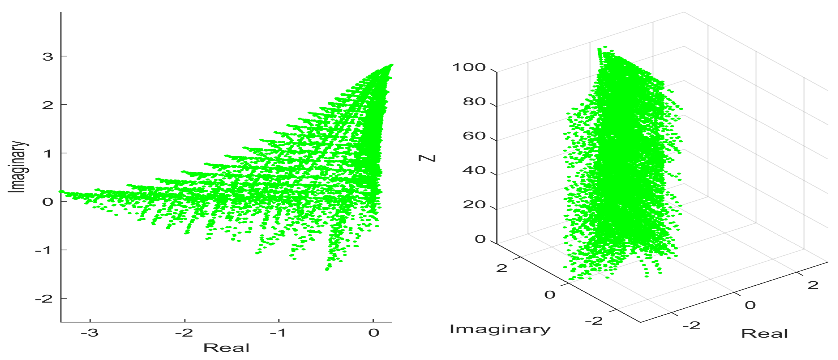
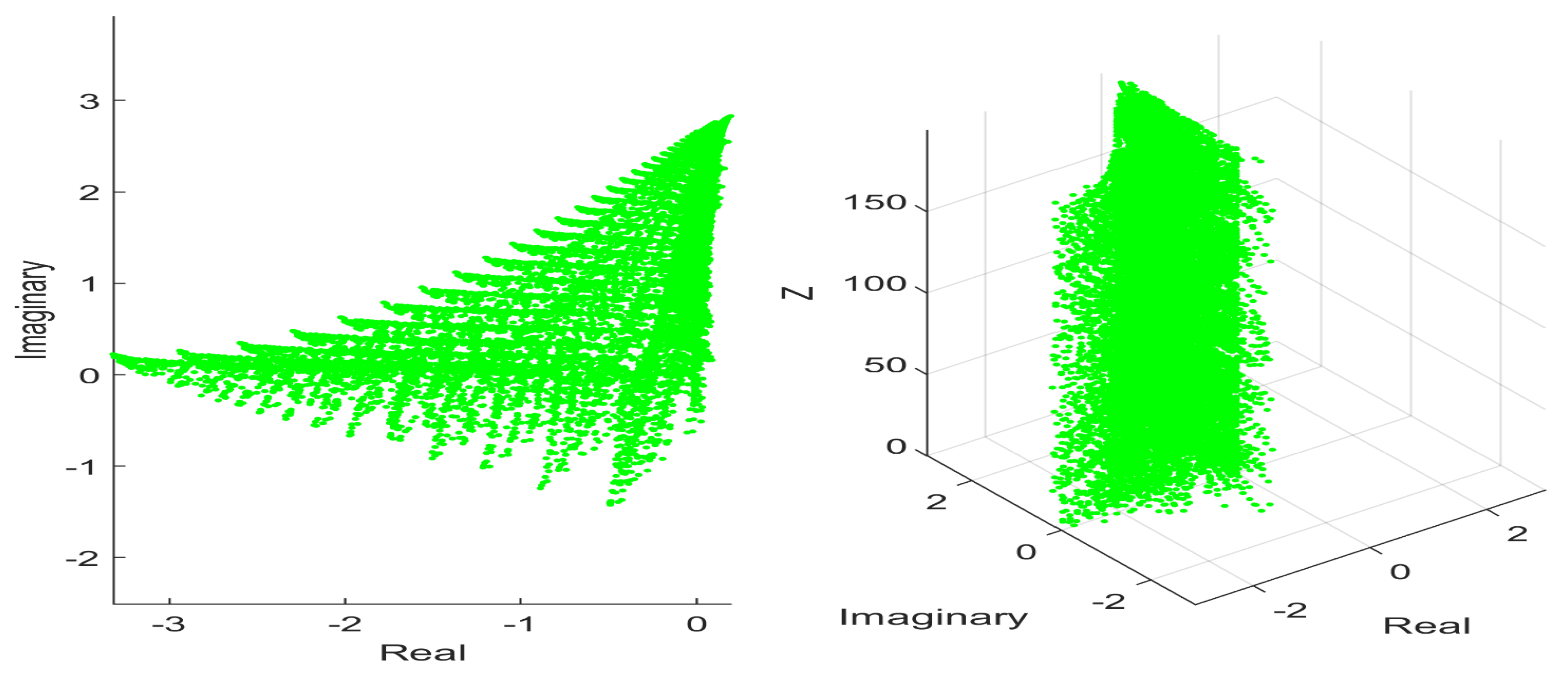
3. Generating the Barnsley Fern Fractal Using a Sequence of Affine Transformations through ${\mathcal{C}}_{\mathit{s}}$-Space

Let $\mathcal{M}=\mathbb{C}$(the set of complex numbers). Consider a sequence defined in $\mathcal{M}$ as follows:

$${\theta }_{2k+1}=\mathcal{H}{\theta }_{2k},$$

where ${\theta }_0$ is an arbitrary complex number in $\mathcal{M}$ and $\mathcal{H}:\mathcal{M}\to \mathcal{M}$ is an affine transformation defined as $\mathcal{H}\theta =\frac{\theta }{2}$, i.e., the affine transformation is a scaling transformation by a factor of $\frac{1}{2}$ applied to each complex number.

To generate a fractal resembling the Barnsley Fern in a ${\mathcal{C}}_s$-space, we need to define complex-valued affine transformations that mimic the transformations used in the construction of the Barnsley Fern fractal. Each transformation will consist of a matrix multiplication and a complex vector addition. Here, we present the complex-valued affine transformations corresponding to the Barnsley Fern:

• Transformation 1:

$${\mathcal{H}}_1=\left(\begin{array}{cc}0& 0\\ 0& 0.16i\end{array}\right)\left(\begin{array}{c}\theta \\ \eta \end{array}\right)+\left(\begin{array}{c}0\\ 0\end{array}\right),$$

with a probability of $0.01$.

• Transformation 2:

$${\mathcal{H}}_2=\left(\begin{array}{cc}0.85& 0.04i\\ -0.04& 0.85\end{array}\right)\left(\begin{array}{c}\theta \\ \eta \end{array}\right)+\left(\begin{array}{c}0\\ 1.6\end{array}\right),$$

with a probability of $0.85$.

• Transformation 3:

$${\mathcal{H}}_3=\left(\begin{array}{cc}0.20i& -0.26\\ 0.23& 0.22i\end{array}\right)\left(\begin{array}{c}\theta \\ \eta \end{array}\right)+\left(\begin{array}{c}0\\ 1.6\end{array}\right),$$

with a probability of $0.07$.

• Transformation 4:

$${\mathcal{H}}_4=\left(\begin{array}{cc}-0.15& 0.28i\\ 0.26i& 0.24\end{array}\right)\left(\begin{array}{c}\theta \\ \eta \end{array}\right)+\left(\begin{array}{c}0\\ 0.44\end{array}\right),$$

with a probability of $0.07$.

Define ${\mathcal{S}}_d:\mathcal{M}\times \mathcal{M}\to \mathbb{C}$ by ${\mathcal{S}}_d(\theta ,\eta )=|\theta -\eta |\mathrm{for}\mathrm{all}\theta ,\eta \in \mathcal{M}$. Clearly, $(\mathcal{M},{\mathcal{S}}_d)$ is ${\mathcal{C}}_s$-space with partial order ≾, as defined in Definition 1.

Define the mapping $\mathcal{O}:\mathcal{M}\to \mathcal{M}$ as the composition of affine transformations as follows:

$$\mathcal{H}(\theta )={\mathcal{H}}_{i_n}\circ {\mathcal{H}}_{i_{n-1}}\circ \dots \circ {\mathcal{H}}_{i_1}(\theta ),$$

where $i_1,i_2,\dots ,i_n$ are randomly chosen indices corresponding to the probabilities associated with each ${\mathcal{H}}_i$. Each ${\mathcal{H}}_i$ is applied to the output of the previous transformation in the sequence. Thus, $\mathcal{O}$ represents the cumulative effect of applying a sequence of affine transformations to the input point $\theta$.

In other words, $\mathcal{O}$ applies a series of transformations determined by the probabilities associated with each ${\mathcal{H}}_i$ to the input point $\theta$. The specific transformation applied at each step depends on the randomly chosen index i according to the associated probabilities. Therefore, $\mathcal{O}$ encapsulates the collective influence of all ${\mathcal{H}}_i$ transformations in generating the fractal pattern.

To highlight the usability of contraction mapping in fractals, for each affine transformation ${\mathcal{H}}_i$, let $L_i$ be its Lipschitz constant. This means that for any two points u and v in $\mathcal{M}$, we have

$$|{\mathcal{H}}_i(u)-{\mathcal{H}}_i(v)|\le L_i|u-v|.$$

Consider two points $\theta ,\eta$ in $\mathcal{M}$. Let $\mathcal{O}(\theta )$ and $\mathcal{O}(\eta )$ be the images of $\theta$ and $\eta$ under the mapping $\mathcal{O}$, respectively.

By the definition of $\mathcal{O}$, we have

$$\mathcal{O}(\theta )={\mathcal{H}}_{i_n}\circ {\mathcal{H}}_{i_{n-1}}\circ \dots \circ {\mathcal{H}}_{i_1}(\theta ),$$

$$\mathcal{O}(\eta )={\mathcal{H}}_{j_m}\circ {\mathcal{H}}_{j_{m-1}}\circ \dots \circ {\mathcal{H}}_{j_1}(\eta ),$$

where $i_1,i_2,\dots ,i_n$ and $j_1,j_2,\dots ,j_m$ are randomly chosen indices corresponding to the probabilities associated with each ${\mathcal{H}}_i$.

Now,

$$\mathcal{O}(\theta )-\mathcal{O}(\eta )=\left({\mathcal{H}}_{i_n}\circ {\mathcal{H}}_{i_{n-1}}\circ \dots \circ {\mathcal{H}}_{i_1}(\theta )\right)-\left({\mathcal{H}}_{j_m}\circ {\mathcal{H}}_{j_{m-1}}\circ \dots \circ {\mathcal{H}}_{j_1}(\eta )\right).$$

We need to show that

$$|\mathcal{O}(\theta )-\mathcal{O}(\eta )|\le L_{max}|\theta -\eta |,$$

where $L_{max}$ is the maximum Lipschitz constant among all $L_i$.

By the Lipschitz continuity of each ${\mathcal{H}}_i$, we have

$$\begin{array}{cc}\hfill |\mathcal{O}(\theta )-\mathcal{O}(\eta )|& =|\left({\mathcal{H}}_{i_n}\circ {\mathcal{H}}_{i_{n-1}}\circ \dots \circ {\mathcal{H}}_{i_1}(\theta )\right)-\left({\mathcal{H}}_{j_m}\circ {\mathcal{H}}_{j_{m-1}}\circ \dots \circ {\mathcal{H}}_{j_1}(\eta )\right)|\hfill \\ \hfill & \le |{\mathcal{H}}_{i_n}\circ {\mathcal{H}}_{i_{n-1}}\circ \dots \circ {\mathcal{H}}_{i_1}(\theta )-{\mathcal{H}}_{j_m}\circ {\mathcal{H}}_{j_{m-1}}\circ \dots \circ {\mathcal{H}}_{j_1}(\eta )|\hfill \\ \hfill & \le L_{max}|\theta -\eta |\hfill \\ \hfill & \le k|\theta -\eta |,\hfill \end{array}$$

where $k=L_{max}=max\{L_1,L_2,L_3,L_4\}$ and ${\mathcal{H}}_i$ is the affine transformation corresponding to each step in the Barnsley Fern fractal generation process, where $i=1,2,3,4$.

The Lipschitz constants of these affine transformations must be taken into account to determine the contraction factor k for the map $\mathcal{O}:\mathcal{M}\to \mathcal{M}$, which is characterized as the composite of affine transformations that describes the Barnsley Fern fractal.

The Lipschitz constant $L_i$ for each of the affine transformation ${\mathcal{H}}_i$ will be written as follows: $i=1,2,3,4$. The greatest Lipschitz constant, or  $L_{max}$, between all conceivable transformations is what we are trying to find.

Each affine transformation ${\mathcal{H}}_i$ has a   $L_i$ that is dependent on its particular attributes. These characteristics comprise the translations, rotation angles, and scaling factors used in the transformation.

Let us utilize the affine transformation ${\mathcal{H}}_2$ as an example.

$${\mathcal{H}}_2=\left(\begin{array}{cc}0.85& 0.04i\\ -0.04& 0.85\end{array}\right)\left(\begin{array}{c}\theta \\ \eta \end{array}\right)+\left(\begin{array}{c}0\\ 1.6\end{array}\right).$$

To estimate its Lipschitz constant, we need to compute the maximum absolute value of the elements of the transformation matrix:

$$\parallel {\mathcal{H}}_2\parallel =max\{|0.85|,|0.04i|,|-0.04|,|0.85|\}.$$

Similarly, we compute the Lipschitz constants $L_1,L_3,L_4$ for the other affine transformations ${\mathcal{H}}_1,{\mathcal{H}}_3,{\mathcal{H}}_4$.

Finally, we determine the maximum Lipschitz constant $L_{max}$ among all $L_1,L_2,L_3,L_4$.

Once we have the maximum Lipschitz constant $L_{max}$, the contraction factor k can be estimated as follows:

$$k=0.85.$$

This estimate ensures that the mapping $\mathcal{O}$ is a contraction mapping with contraction factor $k<1$, satisfying the conditions of Corollary 2. Hence, $\mathcal{O}$ has a unique fixed point that assures the correctness of the fractal generation process. The existence and uniqueness guarantee the convergence and stability of the iterative process, ensuring the accurate generation of fractal patterns.

The provided 2D and 3D visualizations depict the Barnsley Fern fractal, providing captivating observations of its complex arrangement in several dimensions. (See Figure 5, Figure 6, Figure 7, and Figure 8) Through numerous iterations, each point in the fractal pattern emerges as a result of the cumulative application of affine transformations, dynamically evolving based on randomly selected probabilities. In the 2D plot, the fractal sprawls across the complex plane, its delicate fern-like silhouette unfolding with increasing iterations. Meanwhile, in the 3D representation, the fractal extends along the z-axis, creating a mesmerizing volumetric form that showcases the depth and complexity of the pattern. By adjusting the number of iterations, observers can witness the gradual refinement and expansion of the fractal, revealing an ever-growing symphony of shapes and textures within the bounding box constraints.

Figure 5. Two-Dimensional and Three-Dimensional Plots of Barnsley Fern Fractal with 1000 iterations.

Figure 6. Two-Dimensional and Three-Dimensional Plots of Barnsley Fern Fractal with 5000 iterations.

Figure 7. Two-Dimensional and Three-Dimensional Plots of Barnsley Fern Fractal with 10,000 iterations.

Figure 8. Two-Dimensional and Three-Dimensional Plots of Barnsley Fern Fractal with 20,000 iterations.

The fractal creation Algorithm 2 is applied to acquire points that progressively join up in the formation of the Barnsley Fern fractal design by means of affine transforms. The algorithm starts from a particular point and makes several iterations before coming to a stop based on the set number of steps. For every iteration operation, one arbitrarily selects an affine transform based on the predetermined odds. These transformations prescribe the way every single point is updated, which gives rise to the construction of the complex fern-like structure. Lists that correspond to its $\theta$ as well as $\eta$ fractal dimension are generated from the obtained points. The number of iterations is one control variable that determines how detailed the created fractal is. Of even greater importance is the fact that this algorithm provides insight into the basic geometric concepts that underlie the design of the Barnsley Fern fractal and provides an algebraic basis for how it is algorithmically created.

Algorithm 2 Generation of Barnsley Fern Fractal
Require:  $iterations$: number of iterations
Ensure: X: list of x-coordinates, Y: list of y-coordinates
1: $X\leftarrow [0]$	▹ Initialize list for x-coordinates with starting point (0, 0)
2: $Y\leftarrow [0]$	▹ Initialize list for y-coordinates with starting point (0, 0)
3: for  $i=1$ to $iterations$ do
4:        $prob\leftarrow \mathrm{random}()$	▹ Generate a random probability value between 0 and 1
5:       if  $prob<0.01$ then
6:             $\theta \leftarrow 0$
7:             $\eta \leftarrow 0.16\times Y[i-1]$
8:       else if  $prob<0.86$ then
9:             $\theta \leftarrow 0.85\times X[i-1]+0.04\times Y[i-1]$
10:             $\eta \leftarrow -0.04\times X[i-1]+0.85\times Y[i-1]+1.6$
11:       else if  $prob<0.93$ then
12:             $\theta \leftarrow 0.20\times X[i-1]-0.26\times Y[i-1]$
13:             $\eta \leftarrow 0.23\times X[i-1]+0.22\times Y[i-1]+1.6$
14:       else
15:             $\theta \leftarrow -0.15\times X[i-1]+0.28\times Y[i-1]$
16:             $\eta \leftarrow 0.26\times X[i-1]+0.24\times Y[i-1]+0.44$
17:       end if
18: $X\leftarrow X\cup \{\theta \}$	▹ Adding of x-coordinate to data
19: $Y\leftarrow Y\cup \{\eta \}$	▹ Adding of y-coordinate to data
20: end for return  $X,Y$

4. Solving Complex Nonlinear Integral Equations through Contractive Mappings

In this section, nonlinear mixed Volterra–Fredholm integral equation is considered:

$$u(\theta )=\omega (\theta )+\varrho {\int }_0^T{\Psi }_1(\theta ,\hslash ){\Phi }_1(u(\hslash ))d\hslash +\varkappa {\int }_0^{\theta }{\Psi }_2(\theta ,\hslash ){\Phi }_2(u(\hslash ))d\hslash ,0\le \theta \le T.$$

(5)

In this context, ${\Psi }_1$ and ${\Psi }_2$ are mappings from $[0,T]$ to $\mathbb{C}$, $\omega$ is a function from $[0,T]$ to $\mathbb{C}$, and ${\Phi }_1$ and ${\Phi }_2$ map from $\mathbb{R}$ to $\mathbb{C}$. These functions are characterized as continuous and periodic in the complex domain. Additionally, $\varrho$ and $\varkappa$ represent complex numbers, while u is a complex function to be determined. Refer to [16,17,18] for quadrature algorithms, notions of nonlinear dynamics in [19,20,21,22], and utilization of various novel notions in [21,22].

This section solves the nonlinear mixed Volterra–Fredholm integral problem. Assume that the operator $\mathcal{H}$ is defined by

$$\mathcal{H}(u(\theta ))=\omega (\theta )+\varrho {\int }_0^T{\Psi }_1(\theta ,\hslash ){\Phi }_1(u(\hslash ))d\hslash +\varkappa {\int }_0^{\theta }{\Psi }_2(\theta ,\hslash ){\Phi }_2(u(\hslash ))d\hslash ,0\le \theta \le T.$$

(6)

The existence and uniqueness of the solution to the nonlinear mixed Volterra–Fredholm integral equation are examined in this section.

Let $\mathcal{M}=L_p^2[0,T],a>0$ and, for every $\theta ,\eta \in \mathcal{M}$, let

$${\mathcal{S}}_d(\theta ,\eta )=\underset{\hslash \in [0,T]}{sup}{|\theta (\hslash )-\eta (\hslash )|}^2\sqrt{1+a^2}{e}^{i{tan}^{-1}a},$$

be a complex-valued suprametric, where ${\mathcal{S}}_d:\mathcal{M}\times \mathcal{M}\to \mathbb{C},0\le \hslash \le T$ and $\rho \ge 2$.

Define $\mathcal{H}:\mathcal{M}\to \mathcal{M}$ by

$$\mathcal{H}(u(\theta ))=\omega (\theta )+\varrho {\int }_0^T{\Psi }_1(\theta ,\hslash ){\Phi }_1(u(\hslash ))d\hslash +\varkappa {\int }_0^{\theta }{\Psi }_2(\theta ,\hslash ){\Phi }_2(u(\hslash ))d\hslash ,0\le \theta \le T.$$

(7)

We enumerate the subsequent conjectures for our ease of use:

(H₁).

${\Phi }_1,{\Phi }_2:L_p^2[0,T]\to \mathbb{C}$ are continuous with Lipschitz constants ${\mathcal{G}}_1,{\mathcal{G}}_2$; in other words,

$$\mathrm{for}\mathrm{all}u,v\in L_p^2[0,T]:||{\Phi }_i(u)-{\Phi }_i(v)||\le {\mathcal{G}}_i||u-v||,i=1,2\mathrm{and}\mathcal{G}=max\{{\mathcal{G}}_1,{\mathcal{G}}_2\}.$$

(H₂).

$k_1,k_2:[0,T]\times [0,T]\to \mathbb{C}$ are continuous and $\mathcal{W}=max\{{\mathcal{W}}_1,{\mathcal{W}}_2\}$ such that ${\mathcal{W}}_1$ and ${\mathcal{W}}_2$ are finite numbers, where

$${\mathcal{W}}_1=\sqrt{{\int }_0^T{\int }_0^T{|k_1(\theta ,\hslash )|}^{2}d\theta d\hslash }\mathrm{and}{\mathcal{W}}_2=\sqrt{{\int }_0^T{\int }_0^T{|k_2(\theta ,\hslash )|}^{2}d\theta d\hslash }.$$

(H₃).

${|\varrho |}^2+{|\varkappa |}^2<\frac{1}{{\mathcal{G}}^2{\mathcal{W}}^2}$, where $\varrho$ and $\varkappa$ are complex numbers.

Theorem 2.

Let $(\mathcal{M},{\mathcal{S}}_d)$ be a ${\mathcal{C}}_s$-space defined as above. Assuming hypotheses $(H_1)–(H_3)$ are satisfied, there exists a unique solution $u_0(\hslash )$ to Equation (5) over the interval $[0,T]$, and this holds for every $u\in L_p^2[0,T]$.

Proof. 

For $u,v\in L_p^2[0,T]$, we have

$$\begin{array}{cc}\hfill & {|\mathcal{H}(u)-\mathcal{H}(v)|}^2\sqrt{1+a^2}{e}^{i{tan}^{-1}a}\hfill \\ \hfill & =|\omega (\theta )+\varrho {\int }_0^T{\Psi }_1(\theta ,\hslash ){\Phi }_1(u(\hslash ))d\hslash +\varkappa {\int }_0^{\theta }{\Psi }_2(\theta ,\hslash ){\Phi }_2(u(\hslash ))d\hslash \hfill \\ \hfill & -\omega (\theta )-\varrho {\int }_0^T{\Psi }_1(\theta ,\hslash ){\Phi }_1(v(\hslash ))d\hslash -\varkappa {\int }_0^{\theta }{\Psi }_2(\theta ,\hslash ){\Phi }_2(v(\hslash ))d\hslash {|}^2\sqrt{1+a^2}{e}^{i{tan}^{-1}a}\hfill \\ \hfill & =|\varrho {\int }_0^T{\Psi }_1(\theta ,\hslash )({\Phi }_1(u(\hslash ))-{\Phi }_1(v(\hslash )))d\hslash +\varkappa {\int }_0^{\theta }{\Psi }_2(\theta ,\hslash )({\Phi }_2(u(\hslash ))-{\Phi }_2(v(\hslash )))d\hslash {|}^2\sqrt{1+a^2}{e}^{i{tan}^{-1}a}\hfill \\ \hfill & =\left[\frac{1}{T}{\int }_0^T\left(|\varrho {\int }_0^T{\Psi }_1(\theta ,\hslash )({\Phi }_1(u(\hslash ))-{\Phi }_1(v(\hslash )))d\hslash +\varkappa {\int }_0^{\theta }{\Psi }_2(\theta ,\hslash )({\Phi }_2(u(\hslash ))-{\Phi }_2(v(\hslash )))d\hslash {|}^2\right)d\theta \right]\hfill \\ \hfill & \times \sqrt{1+a^2}{e}^{i{tan}^{-1}a}\hfill \\ \hfill & \le \left[\frac{1}{T}\right({|\varrho |}^2{\int }_0^T|{\Psi }_1{(\theta ,\hslash )|}^2|{\Phi }_1(u(\hslash ))-{\Phi }_1{(v(\hslash ))|}^{2}d\hslash +{|\varkappa |}^2{\int }_0^{\theta }|{\Psi }_2{(\theta ,\hslash )|}^2{|{\Phi }_2(u(\hslash ))-{\Phi }_2(v(\hslash ))|}^{2}d\hslash \hfill \\ \hfill & +2|\varrho ||\varkappa |{\int }_0^T|{\Psi }_1(\theta ,\hslash )||{\Phi }_1(u(\hslash ))-{\Phi }_1(v(\hslash ))|d\hslash {\int }_0^{\theta }|{\Psi }_2(\theta ,\hslash )||{\Phi }_2(u(\hslash ))-{\Phi }_2(v(\hslash ))|d\hslash \left)d\theta \right]\hfill \\ \hfill & \times \sqrt{1+a^2}{e}^{i{tan}^{-1}a}\hfill \end{array}$$

$$\begin{array}{cc}\hfill & \le [\frac{1}{T}{|\varrho |}^2{\int }_0^T{\int }_0^T|{\Psi }_1{(\theta ,\hslash )|}^{2}d\hslash d\theta {\int }_0^T{|{\Phi }_1(u(\hslash ))-{\Phi }_1(v(\hslash ))|}^{2}d\hslash \hfill \\ \hfill & +\frac{1}{T}{|\varkappa |}^2{\int }_0^T{\int }_0^T|{\Psi }_2{(\theta ,\hslash )|}^{2}d\hslash d\theta {\int }_0^T{|{\Phi }_2(u(\hslash ))-{\Phi }_2(v(\hslash ))|}^{2}d\hslash \hfill \\ \hfill & +\frac{1}{T}2|\varrho ||\varkappa |\left({\int }_0^T{\int }_0^T|{\Psi }_1{(\theta ,\hslash )|}^{2}d\hslash d\theta {\int }_0^T|{\Phi }_1(u(\hslash ))-{\Phi }_1(v(\hslash ))|d\hslash \right)\hfill \\ \hfill & \times \left({\int }_0^T{\int }_0^T|{\Psi }_2{(\theta ,\hslash )|}^{2}d\hslash d\theta {\int }_0^T|{\Phi }_2(u(\hslash ))-{\Phi }_2(v(\hslash ))|d\hslash \right)]\sqrt{1+a^2}{e}^{i{tan}^{-1}a}\hfill \\ \hfill & \le [\frac{1}{T}{|\varrho |}^2{\mathcal{W}}_1^2{\int }_0^T|{\Phi }_1(u(\hslash ))-{\Phi }_1{(v(\hslash ))|}^{2}d\hslash +\frac{1}{T}{|\varkappa |}^2{\mathcal{W}}_2^2{\int }_0^T{|{\Phi }_2(u(\hslash ))-{\Phi }_2(v(\hslash ))|}^{2}d\hslash \hfill \\ \hfill & +\frac{2}{T}|\varrho ||\varkappa |{\mathcal{W}}_1^2{\mathcal{W}}_2^2{\int }_0^T|{\Phi }_1(u(\hslash ))-{\Phi }_1(v(\hslash ))|d\hslash {\int }_0^T|{\Phi }_2(u(\hslash ))-{\Phi }_2(v(\hslash ))|d\hslash ]\sqrt{1+a^2}{e}^{i{tan}^{-1}a}\hfill \\ \hfill & \le [\frac{1}{T}{|\varrho |}^2{\mathcal{W}}_1^2{\mathcal{G}}_1^2{\int }_0^T{|u(\hslash )-v(\hslash )|}^{2}d\hslash +\frac{1}{T}{|\varkappa |}^2{\mathcal{W}}_2^2{\mathcal{G}}_2^2{\int }_0^T{|u(\hslash )-v(\hslash )|}^2\hfill \\ \hfill & +\frac{2}{T}|\varrho ||\varkappa |{\mathcal{W}}_1^2{\mathcal{W}}_2^2{\mathcal{G}}_1{\mathcal{G}}_2{\int }_0^T{|u(\hslash )-v(\hslash )|}^2]\sqrt{1+a^2}{e}^{i{tan}^{-1}a}\hfill \\ \hfill & =[{|\varrho |}^2{\mathcal{W}}_1^2{\mathcal{G}}_1^2{|u(\hslash )-v(\hslash )|}^2+{|\varkappa |}^2{\mathcal{W}}_2^2{\mathcal{G}}_2^2{|u(\hslash )-v(\hslash )|}^2\hfill \\ \hfill & +2|\varrho ||\varkappa |{\mathcal{W}}_1^2{\mathcal{W}}_2^2{\mathcal{G}}_1{\mathcal{G}}_2{|u(\hslash )-v(\hslash )|}^2]\sqrt{1+a^2}{e}^{i{tan}^{-1}a}\hfill \\ \hfill & \le [{|\varrho |}^2{\mathcal{W}}^2{\mathcal{G}}^2{|u(\hslash )-v(\hslash )|}^2+{|\varkappa |}^2{\mathcal{W}}^2{\mathcal{G}}^2{|u(\hslash )-v(\hslash )|}^2\hfill \\ \hfill & +2|\varrho ||\varkappa |{\mathcal{W}}^2{\mathcal{G}}^2{|u(\hslash )-v(\hslash )|}^2]\sqrt{1+a^2}{e}^{i{tan}^{-1}a}\hfill \\ \hfill & =\left[(|\varrho |+{|\varkappa |)}^2{\mathcal{W}}^2{\mathcal{G}}^2{|u(\hslash )-v(\hslash )|}^2\right]\sqrt{1+a^2}{e}^{i{tan}^{-1}a}\hfill \\ \hfill & \le \left[(|\varrho |+{|\varkappa |)}^2{\mathcal{W}}^2{\mathcal{G}}^2\right]\underset{\hslash \in [0,T]}{sup}{|u(\hslash )-v(\hslash )|}^2\sqrt{1+a^2}{e}^{i{tan}^{-1}a}.\hfill \end{array}$$

Thus,

$$\underset{\hslash \in [0,T]}{sup}|\mathcal{H}(u(\hslash ))-\mathcal{H}(v(\hslash ))|\sqrt{1+a^2}{e}^{i{tan}^{-1}a}\precsim \left[{(|\varrho |}^2+{|\varkappa |}^2){\mathcal{W}}^2{\mathcal{G}}^2\right]{\mathcal{S}}_d(u(\hslash ),v(\hslash )).$$

$$\Rightarrow {\mathcal{S}}_d(\mathcal{H}(u(\hslash ))-\mathcal{H}(v(\hslash )))\precsim L.{\mathcal{S}}_d(u(\hslash ),v(\hslash )),\mathrm{where},L=\left[{(|\varrho |}^2+{|\varkappa |}^2){\mathcal{W}}^2{\mathcal{G}}^2\right]<1.$$

Thus, all the conditions of our Theorem 2 are satisfied. Hence, the mixed Volterra–Fredholm integral equation has a unique solution, which is the unique fixed point.  □

Numerical Illustrations

Example 6.

Consider the mixed Volterra–Fredholm integral equation in a complex plane:

$$u(\theta )=\omega (\theta )+i{\int }_0^{2\pi }\frac{{sin}^2(\hslash )}{15+ln(3+icos(\theta ))}{u}^3(\hslash )d\hslash +{\int }_0^{\theta }\frac{cos(\hslash )}{{(12+sin(\theta ))}^2}u(\hslash )d\hslash ,$$

where $\omega (\theta )$ is such that the exact solution equals $u(\theta )=e^{sin(\theta )}+icos(\theta )$.

Example 7.

Consider the mixed Volterra–Fredholm integral equation in a complex plane:

$$u(\theta )=\omega (\theta )+i{\int }_0^{2\pi }\frac{tan(\hslash )}{10+ln(4+i{e}^{\theta })}{u}^2(\hslash )d\hslash +{\int }_0^{\theta }\frac{e^t}{{(5+tan(\theta ))}^2}u(\hslash )d\hslash ,$$

where $\omega (\theta )$ is such that the exact solution equals $u(\theta )=e^{\theta }+itan(\theta )$.

To compare the approximate and exact solutions for the given nonlinear mixed Volterra–Fredholm integral equation using $m=2$ and $m=16$, we will calculate the numerical solution at specific points $\theta$ and compare it with the exact solution $u(\theta )=e^{\theta }+itan(\theta )$. (See Table 1).

Table 1. Numerical findings concerning the error modulus in Example 4.

$\mathit{\theta }$	m = 2	m = 4	m = 8	m = 16
1	$1.48560\times {10}^{-2}$	$3.50630\times {10}^{-3}$	$2.50720\times {10}^{-4}$	$1.28680\times {10}^{-6}$
2	$1.49940\times {10}^{-2}$	$3.51160\times {10}^{-3}$	$2.50950\times {10}^{-4}$	$1.28795\times {10}^{-6}$
3	$1.49405\times {10}^{-2}$	$3.48470\times {10}^{-3}$	$2.49150\times {10}^{-4}$	$1.27875\times {10}^{-6}$
4	$1.50540\times {10}^{-2}$	$3.50290\times {10}^{-3}$	$2.50340\times {10}^{-4}$	$1.28485\times {10}^{-6}$
5	$1.47810\times {10}^{-2}$	$3.51210\times {10}^{-3}$	$2.51210\times {10}^{-4}$	$1.28930\times {10}^{-6}$
6	$1.48560\times {10}^{-2}$	$3.48740\times {10}^{-3}$	$2.49360\times {10}^{-4}$	$1.27985\times {10}^{-6}$

The exact solution for the given integral equation is

$$u(\theta )=e^{\theta }+itan(\theta ).$$

For the numerical approximation, we solve the integral equation iteratively. Here, we present the approximate solutions for $m=2$ and $m=16$ at specific points $\theta$.

We will compare the exact solution and the approximate solution at different points $\theta$ for $m=2$ and $m=16$.

$\mathbf{\theta }$	Exact Solution	Approximate Solution	Absolute Error	Approximate Solution
	$\mathbf{u}(\mathbf{\theta })={\mathbf{e}}^{\mathbf{\theta }}+\mathbf{i}tan(\mathbf{\theta })$	$\mathbf{m}=\mathbf{2}$	$\mathbf{m}=\mathbf{2}$	$\mathbf{m}=\mathbf{16}$
1	$e+itan(1)\approx 2.718+i1.557$	$2.701+i1.549$	1.48560 × 10−2	$2.718+i1.557$
2	$e^2+itan(2)\approx 7.389+i-2.185$	$7.374+i-2.179$	1.49940 × 10−2	$7.389+i-2.185$
3	$e^3+itan(3)\approx 20.085+i-0.143$	$20.070+i-0.142$	1.49405 × 10−2	$20.085+i-0.143$
4	$e^4+itan(4)\approx 54.598+i1.158$	$54.582+i1.157$	1.50540 × 10−2	$54.598+i1.158$
5	$e^5+itan(5)\approx 148.413+i-3.380$	$148.398+i-3.377$	1.47810 × 10−2	$148.413+i-3.380$
6	$e^6+itan(6)\approx 403.429+i-0.291$	$403.414+i-0.290$	1.48560 × 10−2	$403.429+i-0.291$

•

For $m=2$, the approximate solution deviates more from the exact solution, leading to higher absolute errors;

•

For $m=16$, the approximate solution is very close to the exact solution, resulting in much smaller absolute errors;

•

This demonstrates the improved accuracy of the numerical method with increased iterations, showing the convergence of the method.

The comparison clearly shows that increasing the number of iterations (m) significantly improves the accuracy of the numerical approximation to the exact solution. (See Figure 9). This is consistent with the theoretical expectation that more iterations lead to better convergence in numerical methods for solving integral equations.

Figure 9. Comparison between exact and approximate solutions.

The two subplots provide a detailed visualization of the absolute error in the real and imaginary parts of the solution for the nonlinear mixed Volterra–Fredholm integral equation when using $m=16$ iterations. (See Figure 10). In the left subplot, the red line represents the absolute error in the real part of the solution across the interval $[0,2\pi ]$. This plot illustrates how the numerical approximation closely follows the exact solution, with only minor deviations observable at various points. The right subplot, represented by the blue line, shows the absolute error in the imaginary part of the solution over the same interval. Similar to the real part, the errors in the imaginary part are minimal, indicating a high level of accuracy in the numerical method with $m=16$ iterations. Both subplots highlight the effectiveness of the numerical method, showcasing that increasing the number of iterations significantly reduces the error, thus improving the approximation’s precision.

Figure 10. Error analysis for the real and imaginary components when $m=16$.

5. Discussion and Comparisons

•

The authors of [2] presented complex valued metric spaces and obtained adequate criteria for the existence of a pair of mappings’ common fixed points that meet contractive type requirements. Furthermore, M. Berzig [3] presented the idea of suprametric space and examined some fundamental aspects of its topology quite recently. He then demonstrated the existence of a unique fixed point for specific contraction maps in suprametric spaces. He then used the findings to look into the possibility of finding solutions to specific matrix and nonlinear integral problems.

−

Compared to the above, in this paper, we combined suprametric space and complex-valued metric space to introduce complex-valued suprametric space and presented two non-regular applications, i.e., the Barnsley Fern fractal generation and the solution of mixed Volterra–Fredholm integral equations in the complex plane by using our obtained results in complex-valued suprametric spaces.

•

The authors of [15] investigated an extension of the fixed point theorem for the Kannan contraction on a controlled metric space. This study employed the Kannan contraction on controlled metric spaces to create a novel form of iterated function system, known as CK-IFS. In essence, a controlled metric space was used to construct an iterated function system of Kannan contractions, resulting in the generation of controlled Kannan fractals.

−

Compared to the above, our study delves into the generation of fractals, exemplified by the Barnsley Fern fractal, utilizing sequences of affine transformations within complex-valued suprametric spaces. Furthermore, we present an algorithm for iteratively generating points converging to the Barnsley Fern fractal pattern.

•

A solution to the nonlinear mixed Volterra–integral equations in the complex plane was provided by the authors in [22] using the contraction principle in metric space.

−

Compared to the above, we provided a solution to the nonlinear mixed Volterra–integral equations in the complex plane by using our obtained result in complex-valued suprametric space.

•

Fixed points are useful because many mathematical issues may be expressed in terms of their existence, and it is often faster to establish that they exist and approximate them numerically than to find them explicitly. However, why is our approach important?

−

We utilized a fixed-point approach. This approach has several advantages that make it a preferred choice in many situations:

∗

Our approach is guaranteed to converge to the unique fixed point, whereas other approaches may oscillate or diverge;

∗

The fixed point approach is stable, meaning that small errors in the initial guess or iterations do not propagate and amplify;

∗

The fixed point approach ensures the uniqueness of the solution, whereas other approaches may produce multiple solutions or none at all;

∗

The fixed point approach can be more efficient than other approaches, especially when the contraction factor ℘ is small, as it requires fewer iterations to achieve the desired accuracy.

6. Conclusion and Associated Future Works

In conclusion, this article introduced complex-valued suprametric spaces, showcasing their applicability in various mathematical and algorithmic domains. We demonstrated their effectiveness in quantifying the similarity between fuzzy sets, providing quantitative measures of their relationships. Additionally, we established related fixed oint results, highlighting their relevance in algorithmic and numerical contexts.

Moving forward, future research could explore the application of complex-valued suprametric spaces in other areas of soft computing and mathematical modeling. A deeper understanding of complicated pattern formation may result from more research on the creation of fractals inside these spaces through affine transformations. Additionally, the field of research for complex-valued integral problems could potentially be broadened to include a wider range of difficult and demanding problem domains, opening the door for innovative algorithmic and numerical solutions.

More advanced techniques for fuzzy clustering as well as fractal generation in complex-valued suprametric spaces, in particular, may eventually lead to the creation of more effective and adaptable methods for working with complex and fuzzy data. Furthermore, looking into how these ideas might be used in such fields as artificial intelligence, pattern recognition, and thermogravimetric analysis could lead to new directions in the field of research [23,24,25].

References

- Vass, J. On intersecting IFS fractals with lines. Fractals 2014, 22, 1450014. [Google Scholar] [CrossRef]
- Azam, A.; Fisher, B.; Khan, M. Common Fixed Point Theorems in Complex Valued Metric Spaces. Numer. Funct. Anal. Optim. 2011, 32, 243–253. [Google Scholar] [CrossRef]
- Berzig, M. First Results in Suprametric Spaces with Applications. Mediterr. J. Math. 2022, 19, 226. [Google Scholar] [CrossRef]
- Panda, S.K.; Agarwal, R.P.; Karapınar, E. Extended suprametric spaces and Stone-type theorem. Ext. Suprametric Spaces -Stone-Type Theorem Aims Math. 2023, 8, 23183–23199. [Google Scholar] [CrossRef]
- Panda, S.K.; Abdeljawad, T.; Ravichandran, C. A complex valued approach to the solutions of Riemann-Liouville integral, Atangana-Baleanu integral operator and non-linear Telegraph equation via fixed point method. Chaos Solitons Fractals 2020, 130, 109439. [Google Scholar] [CrossRef]
- Rao, K.; Swamy, P.; Prasad, J. A Common fixed point theorem in complex valued b-metric spaces. Bull. Math. Stat. Res. 2013, 1. [Google Scholar]
- Panda, S.K.; Velusamy, V.; Khan, I.; Niazai, S. Computation and convergence of fixed-point with an RLC-electric circuit model in an extended b-suprametric space. Sci. Rep. 2024, 14, 9479. [Google Scholar] [CrossRef] [PubMed]
- Panda, S.K.; Abdeljawad, T.; Jarad, F. Chaotic attractors and fixed point methods in piecewise fractional derivatives and multi-term fractional delay differential equations. Results Phys. 2023, 46, 106313. [Google Scholar] [CrossRef]
- Rasham, T.; Qadir, R.; Hasan, F.; Agarwal, R.P.; Shatanawi, W. Novel results for separate families of fuzzy-dominated mappings satisfying advanced locally contractions in b-multiplicative metric spaces with applications. J. Inequalities Appl. 2024, 2024, 57. [Google Scholar] [CrossRef]
- Rasham, T.; Asif, A.; Aydi, H.; Sen, M.D.L. On pairs of fuzzy dominated mappings and applications. Adv. Differ. Equ. 2021, 2021, 417. [Google Scholar] [CrossRef]
- Manochehr, K.; Deep, A.; Nieto, J. An existence result with numerical solution of nonlinear fractional integral equations. Math. Methods Appl. Sci. 2023, 46, 10384–10399. [Google Scholar]
- Hammad, H.A.; Aydi, H.; Kattan, D.A. Further investigation of stochastic nonlinear Hilfer-fractional integro-differential inclusions using almost sectorial operators. J. Pseudo-Differ. Oper. Appl. 2024, 15, 5. [Google Scholar] [CrossRef]
- Shagari, M.S.; Alotaibi, T.; Aydi, H.; Aloqaily, A.; Mlaiki, N. New L-fuzzy fixed point techniques for studying integral inclusions. J. Inequalities Appl. 2024, 2024, 83. [Google Scholar] [CrossRef]
- Panda, S.K.; Vijayakumar, V.; Nagy, A.M. Complex-valued neural networks with time delays in the Lp sense: Numerical simulations and finite time stability. Chaos Solitons Fractals 2023, 177, 114263. [Google Scholar] [CrossRef]
- Thangaraj, C.; Easwaramoorthy, D.; Selmi, B.; Chamola, B.P. Generation of fractals via iterated function system of Kannan contractions in controlled metric space. Math. Comput. Simul. 2024, 222, 188–198. [Google Scholar] [CrossRef]
- Dastjerdi, H.L.; Ghaini, F.M. Numerical solution of Volterra–Fredholm integral equations by moving least square method and Chebyshev polynomials. Appl. Math. Model. 2012, 36, 3283–3288. [Google Scholar] [CrossRef]
- Micula, S. On Some Iterative Numerical Methods for Mixed Volterra–Fredholm Integral Equations. Symmetry 2019, 11, 1200. [Google Scholar] [CrossRef]
- Al-Miah, J.T.A.; Taie, A.H.S. A new Method for Solutions Volterra-Fredholm Integral Equation of the Second Kind. J. Phys. Conf. Ser. 2019, 1294, 032026. [Google Scholar] [CrossRef]
- Mashayekhi, S.; Razzaghi, M.; Tripak, O. Solution of the Nonlinear Mixed Volterra-Fredholm Integral Equations by Hybrid of Block-Pulse Functions and Bernoulli Polynomials. Sci. World J. 2014, 2014, 413623. [Google Scholar] [CrossRef]
- Maleknejad, K.; Hadizadeh, M. A new computational method for Volterra-Fredholm integral equations. Comput. Math. Appl. 1999, 37, 1–8. [Google Scholar] [CrossRef]
- Chen, H. Complex Harmonic Splines, Periodic Quasi-Wavelets, Theory and Applications; Kluwer Academic Publishers, 1999. [Google Scholar]
- Beiglo, H.; Gachpazan, M. Numerical solution of nonlinear mixed Volterra-Fredholm integral equations in complex plane via PQWs. Appl. Math. Comput. 2020, 369, 124828. [Google Scholar] [CrossRef]
- Syam, M.M.; Cabrera-Calderon, S.; Vijayan, K.A.; Balaji, V.; Phelan, P.E.; Villalobos, J.R. Mini Containers to Improve the Cold Chain Energy Efficiency and Carbon Footprint. Climate 2022, 10, 76. [Google Scholar] [CrossRef]
- Omari, S.A.; Ghazal, A.M.; Syam, M.; Sayed, H.E.; Najjar, R.A.; Selim, M.Y. An invistigation on the thermal degredation performance of crude glycerol and date seeds blends using thermogravimetric analysis (TGA). In Proceedings of the 2018 5th International Conference on Renewable Energy: Generation and Applications (ICREGA), Al Ain, United Arab Emirates, 25–28 February 2018; pp. 102–106. [Google Scholar] [CrossRef]
- Mourad, A.I.; Ghazal, A.M.; Syam, M.M.; Al Qadi, O.D.; Al Jassmi, H. Utilization of Additive Manufacturing in Evaluating the Performance of Internally Defected Materials. Iop Conf. Ser. Mater. Sci. Eng. 2018, 362, 012026. [Google Scholar] [CrossRef]
Disclaimer/Publisher’s Note: The statements, opinions and data contained in all publications are solely those of the individual author(s) and contributor(s) and not of MDPI and/or the editor(s). MDPI and/or the editor(s) disclaim responsibility for any injury to people or property resulting from any ideas, methods, instructions or products referred to in the content. |
© 2024 by the authors. Licensee MDPI, Basel, Switzerland. This article is an open access article distributed under the terms and conditions of the Creative Commons Attribution (CC BY) license (https://creativecommons.org/licenses/by/4.0/).