Energy Dissipation Law of the Temporal Variable-Step Fractional BDF2 Scheme for Space–Time-Fractional Cahn–Hilliard Equation

Abstract

A high-order variable-step numerical scheme is formulated for the space–time-fractional Cahn–Hilliard equation, employing the variable-step fractional BDF2 formula. The unique solvability and mass conservation at the discretization setting are established. Subject to the constraint of time-step ratios, i.e., $0.4159\le r_k\le 4.660,$ a careful analysis based on the discrete gradient structure of the fractional BDF2 formula reveals that the proposed scheme adheres to the energy dissipation law. Remarkably, the modified energy exhibits asymptotic compatibility with that of the classical Cahn–Hilliard equation. Moreover, the modified energy dissipation law of the resulting scheme for the space–time-fractional Cahn–Hilliard equation aligns asymptotically with that of the variable-step BDF2 scheme for its classical counterpart. Finally, a few numerical experiments combined with the adaptive method are presented, which confirm the accuracy and efficiency of the proposed scheme.

1. Introduction

The classical Cahn–Hilliard equation describing the dynamics of phase separation and coarsening in binary alloys has extensive applications in image processing [1], multi-phase flow [2,3], and tumor growth simulation [4,5]. The Cahn–Hilliard equation stems from the Ginzburg–Landau free energy functional governed by the $H^{-1}$ gradient flow

$$E\left[\varphi \right]:={\int }_{\Omega }\left({\displaystyle \frac{{ϵ}^2}{2}}{|\nabla \varphi |}^2+F\left(\varphi \right)\right)\mathrm{d}\mathbf{x},$$

(1)

where $\mathbf{x}\in \Omega$ = ${(a,b)}^2\subset {\mathbb{R}}^2,$$F\left(\varphi \right)={\displaystyle \frac{1}{4}}{({\varphi }^2-1)}^2$, and $ϵ$ is an interface width parameter. Taking the variational derivative on $\varphi$ in the $H^{-1}$ norm yields the following Cahn–Hilliard equation:

$$\begin{array}{c}\hfill {\varphi }_t:=\kappa \Delta \mu ,\mu ={\displaystyle \frac{\delta E\left[\varphi \right]}{\delta \varphi }}=-{ϵ}^2\Delta \varphi +f\left(\varphi \right),\mathbf{x}\in \Omega ,0<t\le T,\end{array}$$

(2)

where $f\left(\varphi \right)=F^{\prime }\left(\varphi \right).$ It is easy to check that the classical Cahn–Hilliard equation fulfills two physical properties. One is the conservation of mass, that is,

$$\left(\varphi \right(t,x),1)=\left(\varphi \right(0,x),1),\forall t>0.$$

Another is energy dissipation,

$$\begin{array}{c}\hfill {\displaystyle \frac{d}{dt}}E\left(\varphi \right)=\left({\displaystyle \frac{\delta E}{\delta \varphi }},{\varphi }_t\right)=-{\parallel \nabla \mu \parallel }^2\le 0,\forall t>0,\end{array}$$

where $(.,.)$ is the $L^2$-inner product endowed with the norm $\parallel ·\parallel$.

Fractional derivatives are useful tools. That is, equations involving fractional derivatives are used to stimulate complex systems relating to memory effects or long-ranged interactions. Designing efficient numerical schemes for fractional models has received considerable attention in the research literature [6,7,8,9,10,11,12]. The space–time-fractional Cahn–Hilliard (STFCH) equation characterized by the Caputo derivative and fractional Laplace operator is provided by the following dynamic:

$$\begin{array}{cc}\hfill & {}_0{}^{C}D_t^{\alpha }\varphi =-\kappa {(-\Delta )}^{\beta }\mu ,\mu =-{ϵ}^2\Delta \varphi +f\left(\varphi \right),\mathbf{x}\in \Omega ,t\in (0,T),\end{array}$$

(3)

$$\begin{array}{cc}\hfill & \varphi (\mathbf{x},0)={\varphi }_0\left(\mathbf{x}\right),\mathbf{x}\in \Omega ,\hfill \end{array}$$

(4)

subject to the periodic boundary condition. The Caputo definition, ${}_0{}^{C}D_t^{\alpha }u$, reads

$$\begin{array}{c}\hfill {}_0{}^{C}D_t^{\alpha }u\left(t\right):={\displaystyle \frac{1}{\mathsf{\Gamma }(1-\alpha )}}{\int }_0^t{u}^{\prime }\left(s\right){(t-s)}^{-\alpha }\mathrm{d}s.\end{array}$$

(5)

The fractional Laplacian ${(-\Delta )}^{\beta },\beta \in (0,1)$ is defined by using Fourier decomposition

$${(-\Delta )}^{\beta }u=\sum _{m,n\in \mathbb{Z}}{\nu }^{2\beta }{(m^2+n^2)}^{\beta }{\widehat{u}}_{m,n}{e}^{i\nu (mx+ny)},$$

where $\nu =2\pi /L$, and ${\widehat{u}}_{m,n}$ represents the Fourier coefficients of u.

Recently, significant attention has been directed towards the space-fractional Cahn– Hilliard equation. A rather complete picture regarding the well-posedness and regularity results for the general type of the fractional Cahn–Hilliard equation has been provided in [13]. The Fourier–Galerkin approach was applied for the space-fractional Cahn–Hilliard equation in [14], and the well-posedness and error estimate were demonstrated strictly. An energy-stable variable-step BDF2 scheme was constructed by Zhao and Xue in [15], along with energy dissipation and mass conservation.

Various numerical methods, incorporating linear or quadratic interpolation, have been proposed to approximate the Caputo derivative of order $\alpha$. For instance, the $L1$ formula [16,17] with the order of $2-\alpha$ and the formulas with accuracy of $3-\alpha$ order such as the $L2$- $1_{\sigma }$ formula [18,19] and fractional BDF2 (FBDF2) formula [20] are commonly employed regarding the uniform time meshes.

Notably, certain higher-order numerical methods usually necessitate high regularity of the solutions, while the weak singularity of the fractional operator is not satisfactory in establishing high-accuracy numerical schemes as well as high computational costs [21,22]. There have been efficient and energy-stable numerical methods developed on nonuniform meshes for fractional-phase field models to overcome the singularity. Hou et al. [23] constructed unconditionally stable L1, L1-CN, and L1⁺-CN schemes for the time-fractional Allen–Cahn equation on general meshes by splitting the time-fractional derivative into two parts. In [24], a variable-step $L1$ scheme was devised to satisfy the variational energy decay law for the time-fractional Allen–Cahn equation. Subsequently, in [25] by Liao et al., an energy-stable Crank–Nicolson-type scheme with variable time steps was formulated for the time-fractional Allen–Cahn equation. Furthermore, it was demonstrated that the associated energy decay law gradually converges to compatibility with that of the classical counterpart as $\alpha$ approaches 1. Xue and Zhao [26] conducted a comprehensive convergence analysis for the variable-step L1 approach applied to the time-fractional Cahn–Hilliard model. Liao et al. [27] proposed an asymptotically compatible discrete energy approach for the time-fractional Cahn–Hilliard equation by utilizing the FBDF2 formula on the nonuniform mesh.

Taking into account the above discussion, it is worth noting that the introduction of the fractional derivatives results in difficulties constructing accurate and fast numerical methods. The aim of this paper is to construct a variable-step FBDF2 scheme for the STFCH equation. Our main contributions lie in demonstrating the asymptotically compatible energy dissipation law, which is essential to a long-time simulation. In the numerical implementation, we adapt the adaptive time-stepping strategy [28,29,30] for its ability to capture the temporal multi-scale characteristics during the evolution.

The outline of this paper is provided as follows. In Section 2, we construct the variable-step FBDF2 scheme for the STFCH equation. Subsequently, the properties of the proposed scheme are studied in Section 3, incorporating both the unique solvability and the discrete variational energy dissipation law. Several numerical examples are presented in Section 4. A brief conclusion is drawn in Section 5.

2. Variable-Step FBDF2 Numerical Scheme

In this section, a high-order numerical scheme is constructed on nonuniform grids for the STFCH equation by virtue of the variable-step FBDF2 formula (7) and Fourier pseudo-spectral method for temporal and spatial discretization, respectively.

2.1. Fourier Pseudo-Spectral Method

Let M be an even positive integer. We assume that the domain is provided by $\Omega$ = ${(0,L)}^2$, the mesh size $M_x=M_y=:M$, and $M·h=1$. We discretize the spatial variable on the following spatial grid ${\overline{\Omega }}_h:=\{{\mathrm{x}}_h=(x_l,y_j)\}$ with grid points $(x_l,y_j)$ defined by $x_l=lh,y_j=jh,0\le l,j\le M$.

Denote the L-periodic grid function space as ${\mathbb{U}}_h:=\left\{u\right|u=\left(u_h\right)\mathrm{for}{\mathbf{x}}_h\in {\overline{\Omega }}_h\}.$ Let $\overline{Id}=\left\{(m,n)\in {\mathbb{Z}}^2|1\le m,n\le M\right\}$ be an index set; for any $u,v\in {\mathbb{U}}_h,$ the discrete $L^2$ inner product and norm are defined by

$$〈u,v〉=h^2\sum _{(m,n)\in \overline{Id}}{u}_h{v}_h\mathrm{and}∥u∥=\sqrt{〈u,u〉}.$$

Similarly, we deduce the $L^q$-norm in the sequence ${∥u∥}_{l^q}=\sqrt[q]{h^2{\sum }_{(m,n)\in \overline{Id}}{\left|u_h\right|}^q},u\in {\mathbb{U}}_h.$ Since the FCH model is viewed as $H^{-\alpha }$ gradient flow, it is natural to introduce the $H^{-\beta }$ inner product and the associated $H^{-\beta }$-norm ${\parallel ·\parallel }_{-\beta }$

$${\langle u,v\rangle }_{-\beta }=\langle {(-{\Delta }_h)}^{-\beta }u,v\rangle ,{\parallel u\parallel }_{-\beta }=\sqrt{{\langle u,u\rangle }_{-\beta }}.$$

Then, we apply the Fourier pseudo-spectral method to approximate the solution $u(x,y,t)$

$$u(x,y,t)=\sum _{(m,n)\in \widehat{Id}}{\tilde{u}}_{m,n}{e}^{i\nu (mx+ny)},$$

where the novel index set $\widehat{Id}$ is defined as

$$\widehat{Id}=\left\{(m,n)\in {\mathbb{Z}}^2|-{\displaystyle \frac{M}{2}}+1\le m,n\le {\displaystyle \frac{M}{2}}\right\}$$

and the pseudo-spectral coefficients are generated by

$${\tilde{u}}_{m,n}=h^2\sum _{l=0}^{M-1}\sum _{j=0}^{M-1}u(x_l,y_j,t)e^{i\nu (m{x}_l+n{y}_j)}.$$

A straightforward calculation leads to the first- and second-order derivatives of u, which read

$${\mathcal{D}}_x{u}_h=\sum _{(m,n)\in \widehat{Id}}\left(i\nu m\right){\tilde{u}}_{m,n}{e}^{i\nu (m{x}_l+n{y}_j)},{\mathcal{D}}_x^2{u}_h=\sum _{(m,n)\in \widehat{Id}}{\left(i\nu m\right)}^2{\tilde{u}}_{m,n}{e}^{i\nu (m{x}_l+n{y}_j)},$$

$${\mathcal{D}}_y{u}_h=\sum _{(m,n)\in \widehat{Id}}\left(i\nu n\right){\tilde{u}}_{m,n}{e}^{i\nu (m{x}_l+n{y}_j)},{\mathcal{D}}_y^2{u}_h=\sum _{(m,n)\in \widehat{Id}}{\left(i\nu n\right)}^2{\tilde{u}}_{m,n}{e}^{i\nu (m{x}_l+n{y}_j)}.$$

In turn, the discrete gradient operator and Laplace operator are provided by ${\nabla }_h{u}_h={({\mathcal{D}}_x{u}_h,{\mathcal{D}}_y{u}_h)}^T$ and ${\Delta }_h{u}_h=({\mathcal{D}}_x^2+{\mathcal{D}}_y^2)u_h.$

Finally, we define the mean-zero space ${\mathring{\mathbb{U}}}_h=\{u\in {\mathbb{U}}_h|\langle u,1\rangle =0\}.$ For any grid function $u\in {\mathring{\mathbb{U}}}_h$ and $\beta \in \mathbb{R},$ the fractional Laplace operator ${\left(-{\Delta }_h\right)}^{\beta }$ is discretized as follows:

$$\begin{array}{c}\hfill {(-{\Delta }_h)}^{\beta }{u}_h=\sum _{(m,n)\in \widehat{Id}}{\nu }^{2\beta }{(m^2+n^2)}^{\beta }{\tilde{u}}_{m,n}{e}^{i\nu (m{x}_l+n{y}_j)}.\end{array}$$

(6)

Lemma 1 

([15]). For any grid function $u\in {\mathring{\mathbb{U}}}_h,$ it holds the following inequality with $\beta <\delta ,$

$$\begin{array}{c}\hfill {\parallel u\parallel }^2\le {\nu }^{\beta -\delta }\parallel {(-{\Delta }_h)}^{{\displaystyle \frac{\delta }{2}}}{u\parallel ·\parallel u\parallel }_{-\beta }.\end{array}$$

Lemma 2 

([14]). For any grid functions $u,v\in {\mathring{\mathbb{U}}}_h,p,q\ge 0$, it holds that

$$\begin{array}{c}\hfill \langle {(-{\Delta }_h)}^{p+q}u,v\rangle =\langle {(-{\Delta }_h)}^{p}u,{(-{\Delta }_h)}^{q}v\rangle .\end{array}$$

2.2. Fully Discrete Scheme

For a positive integral $N,$ consider the nonuniform temporal grid ${\Omega }_{\tau }$, which is defined by the time levels $0=t_0<t_1<t_2<\cdots <t_N=T$, with the time-step size and adjacent time-step ratio denoted as ${\tau }_k=t_k-t_{k-1}$ and $r_k={\tau }_k/{\tau }_{k-1}$ for $k\ge 2,$ respectively. For any time sequence ${\left\{{\psi }^k\right\}}_{k=0}^N\in {\Omega }_{\tau }$, introduce the difference ${\nabla }_{\tau }{\psi }^k={\psi }^k-{\psi }^{k-1}$. Consequently, the differential quotients are defined by ${\partial }_{\tau }{\psi }^k={\nabla }_{\tau }{\psi }^k/{\tau }_k.$

Points $(t_{j-2},\upsilon \left(t_{j-2}\right)),(t_{j-1},\upsilon \left(t_{j-1}\right))$, and $(t_j,\upsilon \left(t_j\right))$ are used for constructing the interpolating polynomial ${\mathsf{\Pi }}_{2,j}\upsilon \left(t\right)$ in the interval $[t_{j-1},t_j](2\le j\le k),$ and then the first-order derivative of ${\mathsf{\Pi }}_{2,j}\psi \left(t\right)$ is taken as

$$\begin{array}{c}\hfill {\left({\mathsf{\Pi }}_{2,j}\psi \right)}^{\prime }\left(t\right)={\partial }_{\tau }{\psi }^{j+1}+{\displaystyle \frac{2t-t_j-t_{j+1}}{{\tau }_j+{\tau }_{j+1}}}\left({\partial }_{\tau }{\psi }^{j+1}-{\partial }_{\tau }{\psi }^j\right).\end{array}$$

The variable-step FBDF2 method [27] is provided by

$$\begin{array}{cc}\hfill {\mathcal{D}}_{\tau }^{\alpha }{\psi }^k& ={\psi }^k{\displaystyle \frac{1}{\mathsf{\Gamma }(1-\alpha )}}\left(\sum _{j=1}^{k-1}{\int }_{t_{j-1}}^{t_j}{\left({\mathsf{\Pi }}_{2,j}\psi \right)}^{\prime }\left(s\right){(t_k-s)}^{-\alpha }\mathrm{d}s+{\int }_{t_{k-1}}^{t_k}{\left({\mathsf{\Pi }}_{2,k-1}\psi \right)}^{\prime }\left(s\right){(t_k-s)}^{-\alpha }\mathrm{d}s\right)\hfill \\ \hfill & =\sum _{j=1}^k{b}_{k-j}^{\left(k\right)}{\nabla }_{\tau }{\psi }^j+{\displaystyle \frac{r_k{\lambda }_0^{\left(k\right)}}{1+r_k}}({\nabla }_{\tau }{\psi }^k-r_k{\nabla }_{\tau }{\psi }^{k-1})+\sum _{j=1}^{k-1}{\displaystyle \frac{{\lambda }_{k-j}^{\left(k\right)}({\nabla }_{\tau }{\psi }^{j+1}-r_{j+1}{\nabla }_{\tau }{\psi }^j)}{r_{j+1}(1+r_{j+1})}},k\ge 2,\hfill \end{array}$$

(7)

where the coefficients $\left\{b_{k-j}^{\left(k\right)}\right\}$ and $\left\{{\lambda }_{k-j}^{\left(k\right)}\right\}$ are as follows:

$$b_{k-j}^{\left(k\right)}={\displaystyle \frac{1}{\mathsf{\Gamma }(1-\alpha ){\tau }_j}}{\int }_{t_{j-1}}^{t_j}{(t_k-s)}^{-\alpha }\mathrm{d}s,1\le j\le k,$$

$${\lambda }_{k-j}^{\left(k\right)}={\displaystyle \frac{1}{\mathsf{\Gamma }(1-\alpha ){\tau }_j}}{\int }_{t_{j-1}}^{t_j}{\displaystyle \frac{2s-t_j-t_{j-1}}{{\tau }_j}}{(t_k-s)}^{-\alpha }\mathrm{d}s,1\le j\le k.$$

Inspired by the local–nonlocal splitting technique mentioned in [27], Formula (7) is rewritten as

$$\begin{array}{c}\hfill {\mathcal{D}}_{\tau }^{\alpha }{\psi }^k=\left({\displaystyle \frac{1}{2-\alpha }}{b}_0^{\left(k\right)}+{\displaystyle \frac{r_k{\lambda }_0^{\left(k\right)}}{1+r_k}}\right){\nabla }_{\tau }{\psi }^k-{\displaystyle \frac{r_k^2{\lambda }_0^{\left(k\right)}}{1+r_k}}{\nabla }_{\tau }{\psi }^{k-1}+\sum _{j=1}^k{\widehat{b}}_{k-j}^{\left(k\right)}{\nabla }_{\tau }{\psi }^j,k\ge 2,\end{array}$$

where the kernels $\left\{{\widehat{b}}_{k-j}^{\left(k\right)}\right\}$ are provided by

$$\begin{array}{cc}\hfill & {\widehat{b}}_0^{\left(1\right)}=b_0^{\left(1\right)},{\widehat{b}}_0^{\left(k\right)}={\displaystyle \frac{1-\alpha }{2-\alpha }}{b}_0^{\left(k\right)}+{\displaystyle \frac{{\lambda }_1^{\left(k\right)}}{r_k(1+r_k)}},k\ge 2.\hfill \\ \hfill & {\widehat{b}}_{k-j}^{\left(k\right)}=b_{k-j}^{\left(k\right)}-{\displaystyle \frac{{\lambda }_{k-j}^{\left(k\right)}}{1+r_{j+1}}}+{\displaystyle \frac{{\lambda }_{k-j+1}^{\left(k\right)}}{r_j(1+r_j)}},2\le j\le k-1,k\ge 3,\hfill \\ \hfill & {\widehat{b}}_{k-1}^{\left(k\right)}=b_{k-1}^{\left(k\right)}-{\displaystyle \frac{{\lambda }_{k-1}^{\left(k\right)}}{1+r_2}},k\ge 2.\hfill \end{array}$$

Moreover, we employ the L1 formula to approximate the first-level solution

$$\begin{array}{c}\hfill {\mathcal{D}}_{\tau }^{\alpha }{\psi }^1=b_0^{\left(1\right)}{\nabla }_{\tau }{\psi }^1\mathrm{and}{b}_0^{\left(1\right)}={\displaystyle \frac{1}{\mathsf{\Gamma }(1-\alpha ){\tau }_1}}{\int }_{t_0}^{t_1}{(t_1-s)}^{-\alpha }ds.\end{array}$$

At the point $({\mathrm{x}}_h,t_k),$ we arrive at the following variable-step FBDF2 scheme for the STFCH equation, combined with the Fourier pseudo-spectral method

$$\begin{array}{c}\hfill {\mathcal{D}}_{\tau }^{\alpha }{\varphi }_h^k=-\kappa {(-{\Delta }_h)}^{\beta }{\mu }_h^k,{\mu }_h^k=-{ϵ}^2{\Delta }_h{\varphi }_h^k+f\left({\varphi }_h^k\right),{\varphi }_h^k\in {\Omega }_h\times {\Omega }_{\tau },1\le k\le N.\end{array}$$

(8)

Denote $r^{*}$ as the solution of the equation ${\displaystyle \frac{1}{\alpha }}+(1+{\displaystyle \frac{1}{\alpha }})x-x^{2-{\displaystyle \frac{\alpha }{2}}}=0,\alpha \in (0,1)$. It is easy to verify that $r^{*}>R^{*}=4.660.$ Moreover, the root of the equation $2\sqrt{{\displaystyle \frac{x}{1+x}}}+3={\displaystyle \frac{1}{x^2(1+x)}}$ is denoted by $r_{*}\approx 0.4159.$

To proceed with the discrete energy dissipation law associated with the proposed FBDF2 scheme, the following lemma is introduced, which is interpreted as the discrete gradient structure.

Lemma 3 

([27]). Suppose that the time-step ratio satisfies $r_{*}\le r_k\le r^{*},k\ge 2$, and then the following estimate is valid:

$$\begin{array}{c}\hfill \left({\nabla }_{\tau }{v}^k\right)\left({\mathcal{D}}_{\tau }^{\alpha }{v}^k\right)\ge \mathcal{Q}\left[{\nabla }_{\tau }{v}^k\right]-\mathcal{Q}\left[{\nabla }_{\tau }{v}^{k-1}\right]+{\displaystyle \frac{\mathcal{K}(r_k,r_{k+1},\alpha )}{2\mathsf{\Gamma }(3-\alpha ){\tau }_k^{\alpha }}}{\left({\nabla }_{\tau }{v}^k\right)}^2,k\ge 2,\end{array}$$

where

$$\begin{array}{cc}\hfill & \mathcal{K}(p,q,\alpha )={\displaystyle \frac{2+2(1+\alpha )p-\alpha p^{2-\frac{\alpha }{2}}}{1+q}}-{\displaystyle \frac{\alpha q^{2-\frac{\alpha }{2}}}{1+q}}>0,0\le p,q<r^{*},\hfill \\ \hfill & \mathcal{Q}\left[w^k\right]={\displaystyle \frac{\alpha r_{k+1}^{2-\frac{\alpha }{2}}}{2(1+r_{k+1}){\tau }_k^{\alpha }}}{\displaystyle \frac{w_k^2}{\mathsf{\Gamma }(3-\alpha )}}+{\displaystyle \frac{1}{2}}\sum _{j=1}^{k-1}\left(B_{k-j-1}^{\left(k\right)}-B_{k-j}^{\left(k\right)}\right){\left(\sum _{l=j+1}^k{w}_l\right)}^2+{\displaystyle \frac{1}{2}}{B}_{k-1}^{\left(k\right)}{\left(\sum _{l=1}^k{w}_l\right)}^2,\hfill \\ \hfill & B_0^{\left(k\right)}=2b_0^{\left(k\right)},B_{k-j}^{\left(k\right)}={\widehat{b}}_{k-j}^{\left(k\right)}.\hfill \end{array}$$

3. Solvability and the Energy Dissipation Law

In this section, we demonstrate the unique solvability and the energy stability of the variable-step FBDF2 scheme (8) for the STFCH equation. The following lemma presents that scheme (8) is mass-conservative.

Theorem 1. 

The solutions of numerical scheme (8) preserve the mass; that is,

$$\begin{array}{c}\hfill \langle {\varphi }^k,1\rangle =\langle {\varphi }^0,1\rangle ,1\le k\le N.\end{array}$$

(9)

Proof. 

Taking the discrete inner product of (8) with 1, we derive the following identity with the help of Lemma 2:

$$\begin{array}{c}\hfill \langle {\mathcal{D}}_{\tau }^{\alpha }{\varphi }^l,1\rangle =-\langle \kappa {(-{\Delta }_h)}^{\beta }{\mu }^l,1\rangle =0.\end{array}$$

(10)

Next, we prove equality (9) by using mathematical induction. For $l=1$, it follows from $\langle {\mathcal{D}}_{\tau }^{\alpha }{\varphi }^1,1\rangle =\langle B_0^{\left(1\right)}({\varphi }^1-{\varphi }^0),1\rangle$ that $\langle {\varphi }^1,1\rangle =\langle {\varphi }^0,1\rangle ,$ where $B_0^{\left(1\right)}=a_0^{\left(1\right)}.$ Hence, (9) holds for $k=1.$ Further, assume that (9) holds for $l=2,3,\dots ,k-1$; i.e.,

$$\begin{array}{c}\hfill \langle {\varphi }^l,1\rangle =\langle {\varphi }^0,1\rangle ,1\le l\le k-1.\end{array}$$

Then, for $l=k,$ by the definition of the variable-step FBDF2 formula (7), we obtain

$$\begin{array}{c}\hfill 0=\langle {\mathcal{D}}_{\tau }^{\alpha }{\varphi }^k,1\rangle =\langle {\mathcal{B}}_0^{\left(k\right)}({\varphi }^k-{\varphi }^{k-1}),1\rangle +\sum _{j=1}^{k-1}{\mathcal{B}}_{k-j}^{\left(k\right)}\langle ({\varphi }^j-{\varphi }^{j-1}),1\rangle ,\end{array}$$

(11)

where ${\mathcal{B}}_0^{\left(k\right)}=b_0^{\left(k\right)}+{\displaystyle \frac{r_k^2{\lambda }_0^{\left(k\right)}+{\lambda }_1^{\left(k\right)}}{r_k(1+r_k)}},{\mathcal{B}}_1^{\left(k\right)}={\widehat{b}}_1^{\left(k\right)}-{\displaystyle \frac{r_k^2{\lambda }_0^{\left(k\right)}}{1+r_k}},{\mathcal{B}}_j^{\left(k\right)}={\widehat{b}}_j^{\left(k\right)},2\le j\le k-1.$

A combination of (10) and (11) yields ${\displaystyle \sum _{j=1}^{k-1}}{B}_{k-j}^{\left(k\right)}\langle ({\varphi }^j-{\varphi }^{j-1}),1\rangle =0,$ which implies $\langle {\varphi }^k,1\rangle =\langle {\varphi }^{k-1},1\rangle$ by mathematical induction. This completes the proof of Theorem 1. □

Theorem 2. 

Suppose the time-step size ${\tau }_k<\sqrt[\alpha ]{{\displaystyle \frac{4{ϵ}^2}{\kappa {\nu }^{2\beta -2}\mathsf{\Gamma }(2-\alpha )}}}.$ The variable-step FBDF2 scheme (8) is solvable uniquely.

Proof. 

First, we prove the existence of the solution by utilizing the Brouwer fixed-point theorem. The solution of the variable-step FBDF2 scheme (8) could be recast as the existence of a zero problem for map ${\mathsf{\Pi }}_k:{\mathbb{U}}_h\to {\mathbb{U}}_h$ as follows:

$${\mathsf{\Pi }}_k\left({\omega }_h\right)={\mathcal{B}}_0^{\left(k\right)}{\omega }_h-{\mathcal{L}}_h^{(k-1)}+\kappa {(-{\Delta }_h)}^{\beta }(-{ϵ}^2{\Delta }_h{\omega }_h+f\left({\omega }_h\right)),{\omega }_h\in {\mathbb{U}}_h,$$

where ${\mathcal{L}}_h^{(k-1)}={\mathcal{B}}_0^{\left(k\right)}{\varphi }_h^{(k-1)}-\sum _{j=1}^{k-1}{\mathcal{B}}_{k-j}^{\left(k\right)}{\nabla }_{\tau }{\varphi }_h^j.$ Taking the inner product of ${\mathsf{\Pi }}_k\left(\omega \right)$ with ${(-{\Delta }_h)}^{-\beta }\omega$ and applying Lemma 1 and Cauchy–Schwarz inequality, one obtains

$$\begin{array}{cc}\hfill {\langle {\mathsf{\Pi }}_k\left(\omega \right),\omega \rangle }_{-\beta }& ={\langle {\mathcal{B}}_0^{\left(k\right)}\omega ,\omega \rangle }_{-\beta }-{\langle {\mathcal{L}}^{(k-1)},\omega \rangle }_{-\beta }-\kappa {ϵ}^2\langle {\Delta }_h\omega ,\omega \rangle +\kappa \langle f\left(\omega \right),\omega \rangle \hfill \\ \hfill & ={\mathcal{B}}_0^{\left(k\right)}{\parallel \omega \parallel }_{-\beta }^2-\parallel {\mathcal{L}}^{(k-1)}{\parallel }_{-\beta }·{\parallel \omega \parallel }_{-\beta }+\kappa {ϵ}^2\parallel {\nabla }_h{\omega \parallel }^2+{\kappa (\parallel \omega \parallel }_{l^4}^4-{\parallel \omega \parallel }^2)\hfill \\ \hfill & \ge {\mathcal{B}}_0^{\left(k\right)}{\parallel \omega \parallel }_{-\beta }^2-\parallel {\mathcal{L}}^{(k-1)}{\parallel }_{-\beta }·{\parallel \omega \parallel }_{-\beta }+\kappa {ϵ}^2\parallel {\nabla }_h{\omega \parallel }^2-\kappa {\nu }^{\beta -1}\parallel {\nabla }_h{\omega \parallel ·\parallel \omega \parallel }_{-\beta }\hfill \\ \hfill & \ge \left({\mathcal{B}}_0^{\left(k\right)}-{\displaystyle \frac{\kappa {\nu }^{2\beta -2}}{4{ϵ}^2}}\right){\parallel \omega \parallel }_{-\beta }^2-\parallel {\mathcal{L}}^{(k-1)}{\parallel }_{-\beta }·{\parallel \omega \parallel }_{-\beta }.\hfill \end{array}$$

It follows from ${\tau }_k<\sqrt[\alpha ]{{\displaystyle \frac{4{ϵ}^2}{\kappa {\nu }^{2\beta -2}\mathsf{\Gamma }(2-\alpha )}}}$ that ${\mathcal{B}}_0^{\left(k\right)}-{\displaystyle \frac{\kappa {\nu }^{2\beta -2}}{4{ϵ}^2}}>a_0^{\left(k\right)}-{\displaystyle \frac{\kappa {\nu }^{2\beta -2}}{4{ϵ}^2}}>0.$ Therefore, we can find ${\parallel \omega \parallel }_{-\beta }={\displaystyle \frac{1}{{\mathcal{B}}_0^{\left(k\right)}-\frac{\kappa {\nu }^{2\beta -2}}{4{ϵ}^2}}}{\parallel {\mathcal{L}}^{(k-1)}\parallel }_{-\beta }$ to meet ${\langle {\mathsf{\Pi }}_k\left(\omega \right),\omega \rangle }_{-\beta }\ge 0,$ which results in the existence of the solution ${\omega }_h^{*}$ regarding equation ${\mathsf{\Pi }}_k\left({\omega }_h^{*}\right)=0.$

Now, we proceed to establish the solution’s uniqueness. Let ${\rho }_h$ and ${\chi }_h$ represent the distinct solutions of discrete scheme (8). Introduce ${\xi }_h={\chi }_h-{\rho }_h\ne 0$ and commence with the subsequent equation concerning ${\xi }_h$

$${\mathcal{B}}_0^{\left(k\right)}{\xi }_h+\kappa {(-{\Delta }_h)}^{\beta }(-{ϵ}^2{\Delta }_h{\xi }_h^k+f\left({\chi }_h\right)-f\left({\rho }_h\right))=0.$$

Taking the inner product of the above equality with ${(-{\Delta }_h)}^{-\beta }\xi$, we arrive at

$$\begin{array}{c}\hfill {\mathcal{B}}_0^{\left(k\right)}{\parallel \xi \parallel }_{-\beta }^2+\kappa {ϵ}^2{\parallel {\nabla }_h\xi \parallel }^2+\kappa \langle f\left(\chi \right)-f\left(\rho \right),\xi \rangle =0.\end{array}$$

(12)

For the second term on the left-hand side of the above identity, we have

$$\begin{array}{cc}\hfill \langle f\left(\chi \right)-f\left(\rho \right),\xi \rangle & =\langle {\chi }^2+\chi \rho +{\rho }^2,{\xi }^2\rangle -{\parallel \xi \parallel }^2\hfill \\ \hfill & =\langle {(\omega +{\displaystyle \frac{1}{2}}\rho )}^2+{\displaystyle \frac{3}{4}}{\rho }^2,{\xi }^2\rangle -{\parallel \xi \parallel }^2\hfill \\ \hfill & \ge -{\parallel \xi \parallel }^2.\hfill \end{array}$$

Substituting the above inequality into (12) and using Lemma 1 yields

$$\begin{array}{c}\hfill B_0^{\left(k\right)}{\parallel \xi \parallel }_{-\beta }^2+\kappa {ϵ}^2\parallel {\nabla }_h{\xi \parallel }^2\le {\kappa \parallel \xi \parallel }^2\le \kappa {\nu }^{\beta -1}\parallel {\nabla }_h{\xi \parallel ·\parallel \xi \parallel }_{-\beta }\le \kappa {ϵ}^2\parallel {\nabla }_h{\xi \parallel }^2+{\displaystyle \frac{\kappa {\nu }^{2\beta -2}}{4{ϵ}^2}}{\parallel \xi \parallel }_{-\beta }^2.\end{array}$$

(13)

A direct calculation shows

$$\begin{array}{c}\hfill \left({\mathcal{B}}_0^{\left(k\right)}-{\displaystyle \frac{\kappa {\nu }^{2\beta -2}}{4{ϵ}^2}}\right){\parallel \xi \parallel }_{-\beta }^2\le 0.\end{array}$$

The time-step condition ${\tau }_k<\sqrt[\alpha ]{{\displaystyle \frac{4{ϵ}^2}{\kappa {\nu }^{2\beta -2}\mathsf{\Gamma }(2-\alpha )}}}$, which can be rewritten as ${\mathcal{B}}_0^{\left(k\right)}-{\displaystyle \frac{\kappa {\nu }^{2\beta -2}}{4{ϵ}^2}}>0$, along with the estimate (13), cause a contradiction regarding assumption ${\xi }_h\ne 0$. Thus, the uniqueness of the solution to variable-step FBDF2 scheme (8) is clearly demonstrated. This completes the proof. □

A remarkable property of the proposed scheme (8) for the STFCH Equation (3) is provided in the following lemma. Let $E\left[{\varphi }^k\right]$ denote the discrete counterpart of energy (1), expressed as

$$\begin{array}{c}\hfill E\left[{\varphi }^k\right]:={\displaystyle \frac{{ϵ}^2}{2}}\parallel {\nabla }_h{\varphi }^k{\parallel }^2+{\displaystyle \frac{\kappa }{4}}\parallel {\left|{\varphi }^k\right|}^2-1{\parallel }^2,1\le k\le N.\end{array}$$

Furthermore, denote the modified discrete energy as

$$\begin{array}{c}\hfill {\mathcal{E}}_{\alpha }\left[{\varphi }^0\right]=E\left[{\varphi }^0\right],{\mathcal{E}}_{\alpha }\left[{\varphi }^k\right]={\langle \mathcal{Q}\left[{\nabla }_{\tau }{\varphi }^k\right],1\rangle }_{-\beta }+E\left[{\varphi }^k\right],1\le k\le N.\end{array}$$

Theorem 3. 

Assume that the time-step ratio satisfies $r_{*}\le r_k\le r^{*},k\ge 2$ and the time-step size adheres to

$$\begin{array}{c}\hfill {\tau }_k\le \sqrt[\alpha ]{{\displaystyle \frac{4{ϵ}^2\mathcal{K}(r_k,r_{k+1},\alpha )}{\mathsf{\Gamma }(3-\alpha )\kappa {\nu }^{2\beta -2}}}},\end{array}$$

(14)

and then the solution of the numerical scheme (8) complies with

$${\mathcal{E}}_{\alpha }\left[{\varphi }^k\right]\le {\mathcal{E}}_{\alpha }\left[{\varphi }^{k-1}\right],2\le k\le N.$$

Proof. 

Taking the inner product of the FBDF2 scheme (8) with ${(-{\Delta }_h)}^{-\beta }{\nabla }_{\tau }{\varphi }^k$ provides

$$\begin{array}{c}\hfill {\langle {\mathcal{D}}_{\tau }^{\alpha }{\varphi }^k,{\nabla }_{\tau }{\varphi }^k\rangle }_{-\beta }-\kappa {ϵ}^2\langle {\Delta }_h{\varphi }^k,{\nabla }_{\tau }{\varphi }^k\rangle +\kappa \langle f\left({\varphi }^k\right),{\nabla }_{\tau }{\varphi }^k\rangle =0,k\ge 2.\end{array}$$

(15)

For the time-discrete term on the left-hand side of (15), making use of Lemma 3, we obtain the following estimate:

$$\begin{array}{c}\hfill {\langle {\mathcal{D}}_{\tau }^{\alpha }{\varphi }^k,{\nabla }_{\tau }{\varphi }^k\rangle }_{-\beta }\ge {\langle \mathcal{Q}\left[{\nabla }_{\tau }{\varphi }^k\right],1\rangle }_{-\beta }-{\langle \mathcal{Q}\left[{\nabla }_{\tau }{\varphi }^{k-1}\right],1\rangle }_{-\beta }+{\displaystyle \frac{\mathcal{K}(r_k,r_{k+1},\alpha )}{2\mathsf{\Gamma }(3-\alpha ){\tau }_k^{\alpha }}}{\parallel {\nabla }_{\tau }{\varphi }^k\parallel }_{-\beta }^2.\end{array}$$

(16)

Concurrently, an application of the summation by part along with equality $2a(a-b)=a^2-b^2+{(a-b)}^2$ reveals that

$$\begin{array}{cc}\hfill -\langle {\Delta }_h{\varphi }^k,{\nabla }_{\tau }{\varphi }^k\rangle & =\langle {\nabla }_h{\varphi }^k,{\nabla }_{\tau }{\nabla }_h{\varphi }^k\rangle \hfill \\ \hfill & ={\displaystyle \frac{1}{2}}\left(\parallel {\nabla }_h{\varphi }^k{\parallel }^2-{\parallel {\nabla }_h{\varphi }^{k-1}\parallel }^2\right)+{\displaystyle \frac{1}{2}}{\parallel {\nabla }_{\tau }{\nabla }_h{\varphi }^k\parallel }^2.\hfill \end{array}$$

(17)

Meanwhile, the nonlinear term of (15) could be analyzed as follows:

$$\begin{array}{cc}\hfill \langle f\left({\varphi }^k\right),{\nabla }_{\tau }{\varphi }^k\rangle & =\langle {\left({\varphi }^k\right)}^3-{\varphi }^k,{\varphi }^k-{\varphi }^{k-1}\rangle \hfill \\ \hfill & \ge {\displaystyle \frac{1}{4}}(\parallel |{\varphi }^k{|}^2-1{\parallel }^2-\parallel |{\varphi }^{k-1}{|}^2-1{\parallel }^2)-{\displaystyle \frac{1}{2}}{\parallel {\nabla }_{\tau }{\varphi }^k\parallel }^2.\hfill \end{array}$$

(18)

Inserting (16)–(18) into (15), we obtain

$$\begin{array}{c}\hfill {\mathcal{E}}_{\alpha }\left[{\varphi }^k\right]-{\mathcal{E}}_{\alpha }\left[{\varphi }^{k-1}\right]+{\displaystyle \frac{\mathcal{K}(r_k,r_{k+1},\alpha )}{2\mathsf{\Gamma }(3-\alpha ){\tau }_k^{\alpha }}}\parallel {\nabla }_{\tau }{\varphi }^k{\parallel }_{-\beta }^2+{\displaystyle \frac{\kappa {ϵ}^2}{2}}\parallel {\nabla }_{\tau }{\nabla }_h{\varphi }^k{\parallel }^2\le {\displaystyle \frac{\kappa }{2}}{\parallel {\nabla }_{\tau }{\varphi }^k\parallel }^2.\end{array}$$

(19)

It follows form Lemma 1 and Young’s inequality that

$$\begin{array}{c}\hfill {\displaystyle \frac{\kappa }{2}}\parallel {\nabla }_{\tau }{\varphi }^k{\parallel }^2\le {\displaystyle \frac{\kappa }{2}}{\nu }^{\beta -1}\parallel {\nabla }_{\tau }{\nabla }_h{\varphi }^k\parallel ·\parallel {\nabla }_{\tau }{\varphi }^k{\parallel }_{-\beta }\le {\displaystyle \frac{\kappa {ϵ}^2}{2}}\parallel {\nabla }_{\tau }{\nabla }_h{\varphi }^k{\parallel }^2+{\displaystyle \frac{\kappa {\nu }^{2\beta -2}}{8{ϵ}^2}}{\parallel {\nabla }_{\tau }{\varphi }^k\parallel }_{-\beta }^2.\end{array}$$

Substituting the above inequality into (19) and using time-step condition (14), the desired energy dissipation law is available: ${\mathcal{E}}_{\alpha }\left[{\varphi }^k\right]\le {\mathcal{E}}_{\alpha }\left[{\varphi }^{k-1}\right],2\le k\le N.$ This completes the proof of Theorem 3. □

Remark 1. 

As $\alpha \to 1^{-},\beta \to 1^{-}$, the STFCH equation (8) degenerates to the classical Cahn–Hilliard equation. As $\alpha \to 1^{-},$ it provides ${\widehat{b}}_{k-j}^{\left(k\right)}\to 0$ and $B_{k-j}^{\left(k\right)}\to 0,1\le j\le k.$ Thus, as $\alpha \to 1^{-},\beta \to 1^{-},$ we have

$${\mathcal{E}}_{\alpha }\left[{\varphi }^k\right]\to E\left[{\varphi }^k\right]+{\displaystyle \frac{\sqrt{r_{n+1}}{\tau }_{n+1}}{2\kappa \left(1+r_{n+1}\right)}}{∥{\partial }_{\tau }{\varphi }^n∥}_{-1}^2,$$

This implies that the discrete modified energy is asymptotically compatible with the discrete modified energy for the classical Cahn–Hilliard model [30]. Further, as the solution approaches a steady state, ${\nabla }_{\tau }{\varphi }^n\to 0$ yields ${\mathcal{E}}_{\alpha }\left[{\varphi }^k\right]\to E\left[{\varphi }^k\right]$.

Notably, following Theorem 3, it also holds that the discrete modified energy dissipation law for the variable-step FBDF2 scheme (8) of the STFCH equation is asymptotically compatible with the one for the variable-step BDF2 scheme (8) of its classical counterpart

$${\partial }_{\tau }{\mathcal{E}}_{\alpha }\left[{\varphi }^k\right]\le 0\to {\partial }_{\tau }E\left[{\varphi }^k\right]\le 0,\alpha \to 1^{-},\beta \to 1^{-}.$$

4. Numerical Experiment

This section provides three numerical examples equipped with a simple fixed-point algorithm with the termination error ${10}^{-12}$ to show the effectiveness of the variable-step FBDF2 scheme (8) for STFCH equation. All the numerical tests are performed using the software Matlab 2024a. In particular, the sum-of-exponentials technique [31] is used to expedite the evaluation of the variable-step FBDF2 scheme in this article, where the absolute tolerance error and cut-off time are taken as ${10}^{-12}$ and ${10}^{-12}$.

Example 1. 

To investigate the accaracy in time, we consider the following initial value

$${\varphi }_0\left(\mathrm{x}\right)=sinxcosy.$$

for the STFCH equation on domain $\Omega ={(0,2\pi )}^2$, with parameters $\kappa =1,{ϵ}^2=0.1$, and β = 0.5. The final time is chosen as $T=1$.

Taking $T_1=min\{1/\gamma ,T\}$ and denoting the time mesh N, we adapt a two-stage mixed time grid to overcome the weak singularity near the initial time; that is, graded time meshes on $[0,T_1]$ with $t_k={(k/N_1)}^{\gamma },N_1=\lceil {\displaystyle \frac{N}{T+1-{\gamma }^{-1}}}\rceil \mathrm{for}0\le k\le N_1$, and random time meshes on $[T_1,T]$ with ${\tau }_{N_1+n}=(T-T_1)s_n/{\sum }_{k=1}^{N-N_1}{s}_k$ for $1\le n\le N-N_1$, where $s_k$ represents a random number from 0 to 1. We take M = 500 to obtain the reference solution ${\varphi }^N$ with the uniform time-step size $\tau ={10}^{-4}$. The $L^2$-norm error and temporal convergence order are calculated by

$$\begin{array}{c}\hfill e\left(N\right)=\parallel \varphi \left(t_N\right)-{\varphi }^N\parallel ,Orde{r}_{\tau }={\displaystyle \frac{\log \left(e\right(N)/e(2N\left)\right)}{\log \left(\tau \right(N)/\tau (2N\left)\right)}},\end{array}$$

where $\tau \left(N\right)$ stands for the maximum time-step size. The $L^2$-norm errors and the convergence orders, computed by the proposed numerical scheme (8) with different orders of the Caputo derivative $\alpha =0.6,0.8,0.9$, and $\gamma =1,2,3$, are displayed in

Table 1. Errors and temporal convergence orders of the proposed scheme (8).

$\mathit{\alpha }$	N	$\mathit{e}\left(\mathit{N}\right)$	${\mathbf{Order}}_{\mathit{\tau }}$	$\mathit{e}\left(\mathit{N}\right)$	${\mathbf{Order}}_{\mathit{\tau }}$	$\mathit{e}(\mathit{M},\mathit{N})$	${\mathbf{Order}}_{\mathit{\tau }}$
$0.6$	20	9.09 × ${10}^{-3}$	-	1.17 × ${10}^{-3}$	-	9.92 × ${10}^{-4}$	-
	40	5.35 × ${10}^{-3}$	0.76	2.95 × ${10}^{-4}$	1.59	1.93 × ${10}^{-4}$	2.45
	80	3.12 × ${10}^{-3}$	0.78	1.32 × ${10}^{-4}$	1.60	3.69 × ${10}^{-5}$	2.43
	160	1.81 × ${10}^{-3}$	0.78	4.36 × ${10}^{-5}$	1.60	7.01 × ${10}^{-6}$	2.42
$0.8$	20	9.00 × ${10}^{-2}$	-	2.10 × ${10}^{-2}$	-	3.48 × ${10}^{-2}$	-
	40	6.49 × ${10}^{-2}$	0.47	1.05 × ${10}^{-2}$	1.02	1.26 × ${10}^{-2}$	1.52
	80	4.64 × ${10}^{-2}$	0.48	5.26 × ${10}^{-3}$	1.01	4.47 × ${10}^{-3}$	1.52
	160	3.30 × ${10}^{-2}$	0.49	2.63 × ${10}^{-3}$	1.00	1.58 × ${10}^{-3}$	1.51
$0.9$	20	3.37 × ${10}^{-2}$	-	5.89 × ${10}^{-3}$	-	1.03 × ${10}^{-2}$	-
	40	2.11 × ${10}^{-2}$	0.68	2.44 × ${10}^{-3}$	1.29	2.67 × ${10}^{-3}$	2.02
	80	1.31 × ${10}^{-2}$	0.69	9.63 × ${10}^{-4}$	1.36	6.65 × ${10}^{-4}$	2.04
	160	8.08 × ${10}^{-3}$	0.69	3.71 × ${10}^{-4}$	1.38	1.62 × ${10}^{-4}$	2.06

, respectively. As expected, the variable-step FBDF2 scheme (8) achieves the optimal temporal convergence order $O\left({\tau }^{3-\alpha }\right)$ for suitable grading parameters $\gamma .$

Example 2. 

To verify the discrete energy dissipation law of the STFCH equation in the domain $\Omega ={(0,2\pi )}^2$ with $\kappa =0.1$ and $ϵ=0.05$, the initial condition is taken as

$$\begin{array}{c}\hfill {\varphi }_0\left(\mathrm{x}\right)=0.1\times (2\mathrm{rand}\left(\mathrm{x}\right)-1),\mathrm{x}\in \Omega .\end{array}$$

We set the parameters to be $M=128$ and $T_1=0.01$. The graded mesh is adopted on the initial interval $[0,T_1]$ with $\gamma =3 \mathrm{a}\mathrm{n}\mathrm{d} N_1=30$. Regarding the remainder interval $[T_1,T],$ we choose the adaptive time-stepping strategy [32] rather than random time meshes in Example 1 for its better performance to capture the multi-scale features, which in turn results in improving computational efficiency

$${\tau }_{ada}=max\left\{{\tau }_{min},{\displaystyle \frac{{\tau }_{max}}{\sqrt{1+\eta \parallel {\partial }_{\tau }{u}^n{\parallel }^2}}}\right\},$$

where the minimum and maximum size of time steps ${\tau }_{min}$ and ${\tau }_{max}$ are set to be ${10}^{-1}$ and ${10}^{-3}$, respectively.

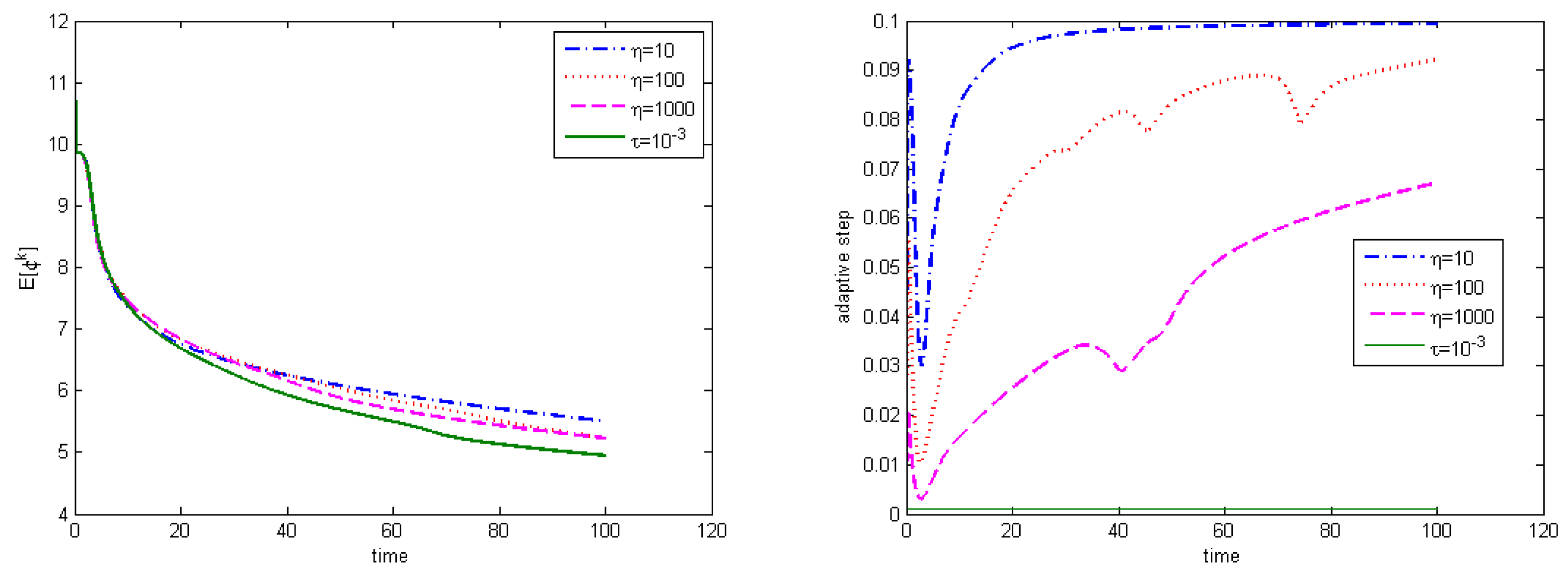
In Figure 1, we consider the case with $T=100,\alpha =0.5,$ and $\beta =0.8$ and plot the evolutions of the discrete energy and the associated time-step sizes with $\eta =10,100,$ and 1000. The relevant result obtained by the uniform time step $\tau ={10}^{-3}$ is also depicted there. It is observed that the value of $\eta$ has an impact on the adaptive time-step sizes, and the discrete energy $E\left[{\varphi }^k\right]$ is closer to the discrete energy computed by the reference solution for the larger $\eta .$

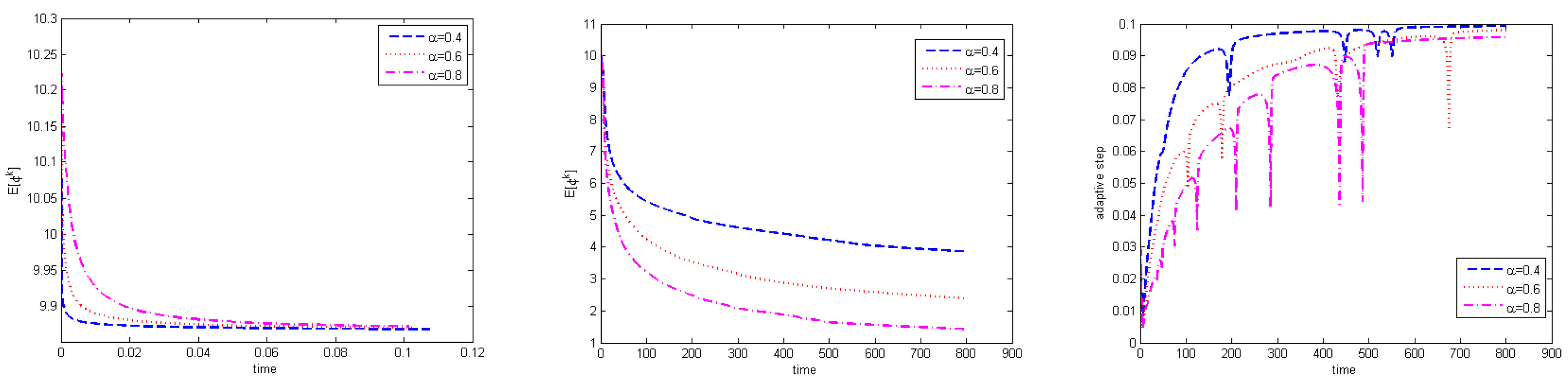
By taking the adaptive parameter $\eta ={10}^3,$ Figure 2 displays the discrete energy evolutions and the variations in adaptive time-step size for $\alpha =0.4,0.6,$ and $0.8$ with $\beta =0.5$. It is shown that the small $\alpha$ leads to the acceleration of the energy decay rate during the initial time interval. Nonetheless, achieving a steady state takes more time computationally for smaller $\alpha .$ The variations in the adaptive time-step size demonstrate the accurate capture of temporal multi-scale energy decay behaviors by the adaptive time-stepping strategy.

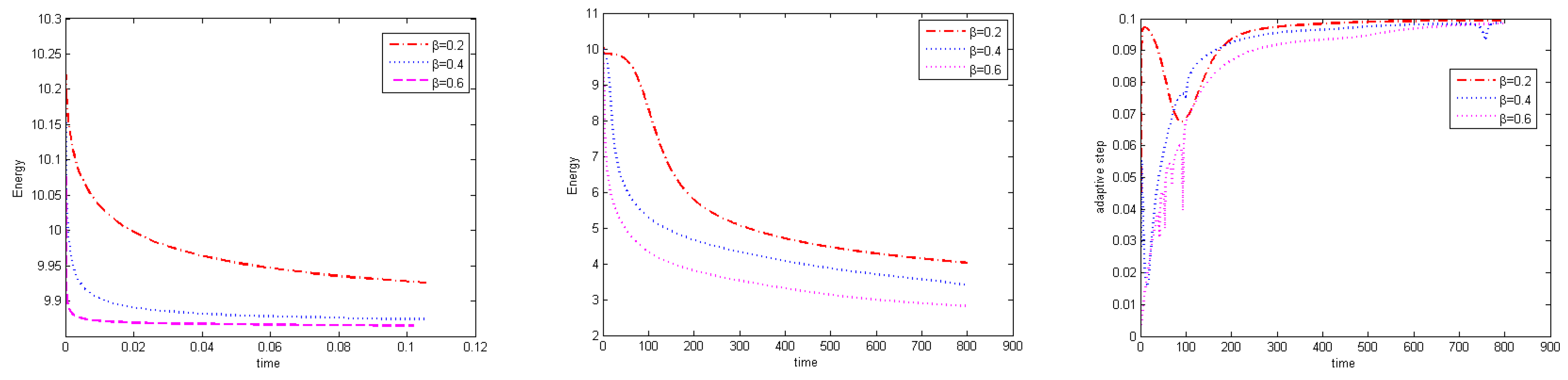
Subsequently, we explore how altering the order $\beta$ impacts the evolution of discrete energy. For this investigation, we fix adaptive parameter $\eta ={10}^3$, $\alpha =0.6$, and set $T=800.$ The discrete energy evolutions and the variations in adaptive time-step size for $\beta =0.4,0.6,0.8$ are plotted in Figure 3. Clearly, as the value of $\beta$ becomes larger, the discrete energy reaches a steady state more rapidly.

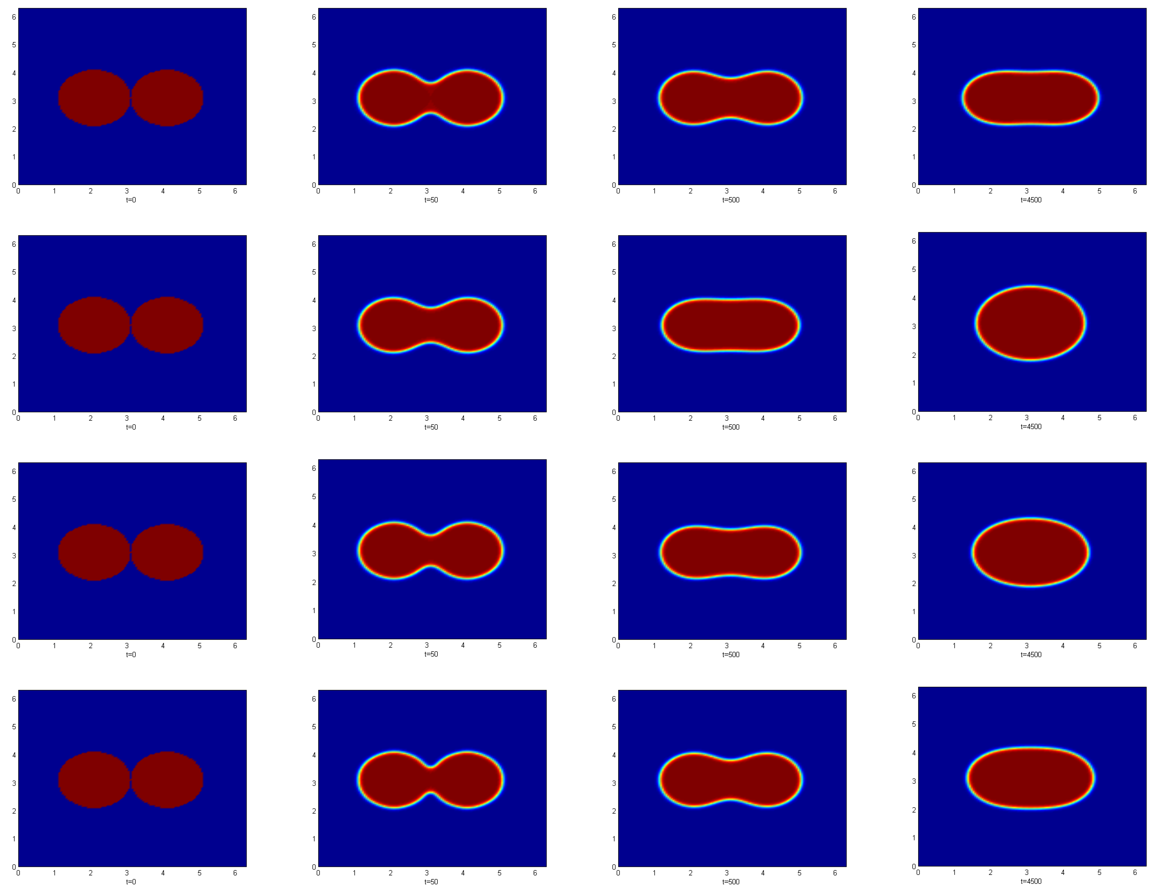
Example 3. 

We study the coarsening dynamics of STFCH equation with $\kappa =0.01$ and $ϵ=0.07$. The initial data for the simulation are provided by

$$\begin{array}{c}\hfill {\varphi }_0(x,y)=\left\{\begin{array}{cc}\hfill & 1,{(x-\pi +1)}^2+{(y-\pi )}^2\le 1,\mathit{or}{(x-\pi -1)}^2+{(y-\pi )}^2\le 1,\hfill \\ \hfill & -1,\mathit{other},\hfill \end{array}\right.\end{array}$$

We set $\Omega ={(0,2\pi )}^2$ with $M=128$. We depict the solutions of the numerical scheme (8) at times t = 0, 50, 500, and 4500 with different orders of the fractional derivatives using the same time meshes in Example 2. Figure 4 presents the condensation of two bubbles. We observe that the speed of condensation is related to the orders of fractional derivatives $\alpha$ and $\beta .$ The larger the values of $\alpha$ and $\beta$ are, the faster the bubbles condense. This is in line with what we observed in Example 2.

5. Conclusions

We presented in this paper the efficient FBDF2 scheme for the STFCH equation on the temporal nonuniform grids. The proposed scheme exhibits the conservation of mass. In addition, the energy dissipation law of the numerical scheme was rigorously demonstrated by means of the discrete gradient structure. The numerical results verified the theoretical results of the proposed scheme. In the future, it is important to explore the properties of the coefficients discretized by the fractional BDF2 method to obtain the convergence of the scheme.