An Error Analysis Study for the Distributed-Order Time-Fraction Model Using an Efficient Numerical Method

Abstract

In this paper, we propose a numerical scheme based on the shifted Legendre polynomials for solving the forced Korteweg–de Vries (fKdV) equation including a Caputo fractional operator of a distributed order. To obtain numerical solutions of these types of equations, we derive an operational matrix based on the shifted Legendre polynomials, and using this operational matrix, their equations change to a set of nonlinear algebraic systems. Then, by calculating these systems in the collocation points, we solve systems. Also, convergence and error are investigated in this paper. Finally, several numerical examples to show the applicability of our scheme are displayed.

1. Introduction

This manuscript studies a numerical method based on an efficient numerical method to solve the following model:

$$\begin{array}{ccc}\hfill {}^C\mathfrak{D}_t^{{\varrho }_{\mu }}u(x,t)+{\displaystyle \frac{1}{2}}{\left(u^2(x,t)\right)}_x+\beta u_{xxx}(x,t)& =& \alpha f_x(x,t),\hfill \\ \hfill u(x,0)& =& u_0\left(x\right),\hfill \end{array}$$

(1)

in which ${}^C\mathfrak{D}_t^{{\varrho }_{\mu }}u(x,t)$ is the distributed-order fractional operator and is defined by

$$\begin{array}{ccc}\hfill {}^C\mathfrak{D}_t^{{\varrho }_{\mu }}u(x,t)& =& {\int }_{{\nu }_1}^{{\nu }_2}{\varrho }_{\mu }{\mathfrak{D}}_t^{\mu }u(x,t)d\mu ,{\nu }_1,{\nu }_2>0,\hfill \end{array}$$

(2)

where ${\varrho }_{\mu }$ is the weight function. Also, in Formula (2), ${\mathfrak{D}}_t^{\mu }u(x,t)$ is the Caputo fractional operator which is defined by [1,2,3,4,5]:

$$\begin{array}{c}\hfill {\mathfrak{D}}_t^{\mu }u(x,t)={\displaystyle \frac{1}{\Gamma (1-\mu )}}{\int }_0^t{\displaystyle \frac{1}{{(t-\tau )}^{\mu }}}{u}_{\tau }(x,\tau )d\tau .\end{array}$$

(3)

The overall shape of a Tsunami propagation equation is given in [6] by

$$\begin{array}{c}\hfill \underset{\eta (x,t)}{\underbrace{{\eta }_t}}+\underset{c\approx {\left(gh\right)}^{{\displaystyle \frac{1}{2}}}}{\underbrace{c{\eta }_x}}+\underset{\alpha ={\displaystyle \frac{3c}{2h_0}}}{\underbrace{\alpha \eta {\eta }_x}}+\underset{\beta ={\displaystyle \frac{c}{6}}{h}_0^2}{\underbrace{\beta {\eta }_{xxx}}}=\underset{f={\displaystyle \frac{-c}{2}}z(x,t)}{\underbrace{f_x}},\end{array}$$

(4)

where $\eta ,z,h,c$ and g are known functions. In this article, we consider the two case for the function $f_x(x,t)$, as follows:

• When in Equation (4), $f_x(x,t)=0$, then the Tsunami propagation Equation (4) changes to a Korteweg–de Vries equation.
• When in Equation (4), $f_x(x,t)\ne 0$, then the Tsunami propagation Equation (4) changes to a forced KdV equation where $f_x(x,t)\ne 0$ is the force part.

By inserting the variable $u(x,t)$ with the value $c+\alpha \eta (x,t)$ in the relation (4), we have

$$\begin{array}{c}\hfill {\displaystyle \frac{\partial u(x,t)}{\partial t}}+{\displaystyle \frac{1}{2}}(u^2{(x,t))}_x+\beta u_{xxx}(x,t)=\alpha f_x(x,t),\end{array}$$

(5)

in which Equation (5) is a hydrodynamic form of the Tsunami generation used to demonstrate the governing equations [7,8]. We can also find different forms of this type of equation in [9,10]. In [8], the authors were able to obtain an analytical solution for this type of equation by considering diverse values of the known function $f(x,t)$. The forced Korteweg–de Vries shows a large multiplicity of nonlinear equations in various fields of physics, chemistry, and engineering. A physical interpretation for this type of model can be considered for the case where the time-fractional operators act on multiple time scales. One of the important applications of the time-fractional model can be considered in a medium in which there is no fixed scaling exponent. For example, we can introduce multi-fractal medium in which there are memory effects on multiple time scales [11]. In this study, we apply a numerical approach based on the shifted Legendre polynomials for solving Equation (2). Also, the obtained numerical approach involves a matrix operator of the distributed-order fractional derivative. One of the important and basic points in this article is that we use the numerical scheme to obtain the solutions of these types of equations using the best approximation. The important applications of these equations can be seen in engineering and physics sciences. For instance, we can refer to the progressive waves that contain nonlinear models [12], oscillations models [13], magnetohydrodynamic [14], transcritical models [15], geostrophic turbulence [16], super thermal plasmas [17], and unmagnetized collisional dusty plasma [18]. Many papers were studied and checked regarding the solutions of fKdV equations by applying the analytical and numerical techniques, for instance, the homotopy approach [19], the differential transform approach [20], the analysis technique based on variational iteration method [21], the analysis technique based on reduced differential transform method [22], the numerical method based on the finite-difference technique [23], the numerical method based on the semi-implicit finite-difference method [24], the spectral collocation method [25,26,27,28].

This paper is organized into the following parts. In Section 2, we describe the lemmas and main preliminaries. Also, this part studies the main property of the Legendre function and shifted Legendre function. In Section 3, we check and obtain an approximation function for solving Equation (1). In Section 4, by applying the approximation function, which is calculated in Section 3, we obtain the approximate solutions of Equation (1). Finally, in Section 5, we display the three numerical examples to show the effectiveness of our method.

2. Preliminaries

This part explains the significant definitions and main lemmas which will applied in the next section.

Definition 1.

For $n\in \mathbb{N}$, the Legendre functions $L_n\left(z\right)$ over the interval $z\in [-1,1]$ are shown by a recurrence formula [29], as follows:

$$\begin{array}{ccc}\hfill L_{n+1}\left(z\right)& =& {\displaystyle \frac{(2n+1)z{L}_n\left(z\right)-n{L}_{n-1}\left(z\right)}{n+1}},\hfill \\ \hfill L_0\left(z\right)& =& 1,L_1\left(z\right)=z.\hfill \end{array}$$

(6)

The analytical form of $L_n\left(z\right)$ can be displayed by

$$\begin{array}{ccc}\hfill L_n\left(z\right)& =& 2^n\sum _{k=0}^{n}n!\left(\begin{array}{c}{\displaystyle \frac{n+k-1}{2}}\\ n\end{array}\right){\displaystyle \frac{z^k}{k!(n-k)!}}.\hfill \end{array}$$

(7)

Definition 2.

The shifted Legendre functions over interval $[0,1]$ are displayed [29] as follows:

$$\begin{array}{cc}\hfill {\mathbb{P}}_{n+1}\left(x\right)& ={\displaystyle \frac{(2n+1)(2x-1){\mathbb{P}}_n\left(x\right)-n{\mathbb{P}}_{n-1}\left(x\right)}{n+1}},n=1,2,\dots ,\hfill \\ \hfill {\mathbb{P}}_0\left(x\right)& ={\mathbb{P}}_1\left(1\right),{\mathbb{P}}_1\left(x\right)=2x-1,\hfill \end{array}$$

(8)

in which ${\mathbb{P}}_n\left(x\right)=L_n(2x-1)$. The analytical form of the above functions can be displayed by the following finite series:

$$\begin{array}{ccc}\hfill {\mathbb{P}}_n\left(x\right)& =& \sum _{k=0}^n{\displaystyle \frac{{(-1)}^{k+n}(k+n)!}{(n-k)!{(k!)}^2}}{x}^k.\hfill \end{array}$$

(9)

Also, the orthogonal properties of ${\mathbb{P}}_n\left(x\right)$ are displayed by

$$\begin{array}{ccc}\hfill {\int }_0^1{\mathbb{P}}_m\left(y\right){\mathbb{P}}_n\left(y\right)dy& =& \left\{\begin{array}{cc}{\displaystyle \frac{1}{2n+1}},& n=m,\\ 0& n\ne m.\end{array}\right.\hfill \end{array}$$

(10)

Lemma 1.

Suppose that $k\ge \lceil \mu \rceil ,k\in \mathbb{N}$. Then, ${\mathfrak{D}}_t^{\mu }{t}^{\xi }$ is calculated as follows [5]:

$$\begin{array}{ccc}\hfill {\mathfrak{D}}_t^{\mu }{t}^k& =& \left\{\begin{array}{cc}0,& k<\lceil \mu \rceil ,\\ {\displaystyle \frac{\Gamma (k+1)}{\Gamma (k+1-\mu )}},t^{k-\mu }& k\ge \lceil \mu \rceil ,\\ 0,& k=0.\end{array}\right.\hfill \end{array}$$

(11)

Lemma 2.

Suppose that $\mathbb{H}\left(t\right),t\in ({\nu }_1,{\nu }_2)$ is a integrable function, then the following relation holds [30]:

$$\begin{array}{c}\hfill {\int }_{{\nu }_1}^{{\nu }_2}\mathbb{F}\left(t\right)dt\simeq \sum _{p=0}^{\mathbf{s}}{\mathbb{W}}_p\mathbb{F}\left({\delta }_p\right),\end{array}$$

(12)

in which ${\delta }_p$ and ${\mathbb{W}}_p$ for $p=1,2,\dots ,s$ are defined by

$$\begin{array}{ccc}\hfill {\delta }_p& =& {\displaystyle \frac{{\nu }_2-{\nu }_1}{2}}{\varsigma }_p+{\displaystyle \frac{{\nu }_2+{\nu }_1}{2}},\hfill \\ \hfill {\mathbb{W}}_p& =& {\displaystyle \frac{{\nu }_2-{\nu }_1}{\left(1-{\varsigma }_p^2\right){\left[L_{\mathbf{s}}^{\prime }\left({\varsigma }_p\right)\right]}^2}},\hfill \end{array}$$

(13)

in which ${\varsigma }_p$ are the roots of $L_s\left(x\right)$.

3. Construction of the Approximate Function

To approximate the function $u(x,t)$ over the interval $L^2[0,1]\times [0,1]$, we consider the infinite series, as follows:

$$\begin{array}{ccc}\hfill u(x,t)& =& \sum _{l_1=0}^{\infty }\sum _{l_2=0}^{\infty }{\mathbb{P}}_{l_1}\left(x\right)u_{l_1{l}_2}{\mathbb{P}}_{l_2}\left(t\right),\hfill \end{array}$$

(14)

in which

$$\begin{array}{c}\hfill u_{ij}=(2i+1)(2j+1){\int }_0^1{\int }_0^1{\mathbb{P}}_j\left(t\right)u(x,t){\mathbb{P}}_i\left(x\right)dxdt.\end{array}$$

(15)

Considering $n+1$-sentence of the above series, we obtain

$$\begin{array}{ccc}\hfill u(x,t)& \simeq u_{nn}=& \sum _{l_1=0}^n\sum _{l_2=0}^n{u}_{l_1{l}_2}{\mathbb{P}}_{l_1}\left(x\right){\mathbb{P}}_{l_2}\left(t\right)={\Phi }^T\left(x\right){\rm Y}\Phi \left(t\right),\hfill \end{array}$$

(16)

in which

$$\begin{array}{c}\hfill \Phi \left(x\right)=\left(\begin{array}{c}{\mathbb{P}}_0\left(x\right)\\ {\mathbb{P}}_1\left(x\right)\\ ⋮\\ {\mathbb{P}}_n\left(x\right)\end{array}\right),\Phi \left(t\right)=\left(\begin{array}{c}{\mathbb{P}}_0\left(t\right)\\ {\mathbb{P}}_1\left(t\right)\\ ⋮\\ {\mathbb{P}}_n\left(t\right)\end{array}\right),\end{array}$$

and ${\rm Y}={\left[u_{l_1{l}_2}\right]}_{(n+1)\times (n+1)}$.

Theorem 1.

For $\mu \in (0,1]$, we obtain

$$\begin{array}{ccc}\hfill {\mathfrak{D}}_t^{\mu }\Phi \left(t\right)& =& \mathit{P}\mathit{Q}(\mu ,t){\Psi }_n\left(t\right),\hfill \end{array}$$

(17)

where

$$\mathit{Q}(\mu ,t)=\left(\begin{array}{ccccc}0& 0& 0& \dots & 0\\ 0& {\displaystyle \frac{1}{\Gamma (2-\mu )}}& 0& \dots & 0\\ 0& 0& {\displaystyle \frac{2}{\Gamma (3-\mu )}}& ⋮& ⋮\\ ⋮& ⋮& ⋮& \ddots & ⋮\\ 0& 0& 0& \dots & {\displaystyle \frac{n!}{\Gamma (n-\mu +1)}}\end{array}\right)t^{-\mu },$$

$$\mathit{P}=\left(\begin{array}{ccccc}1& 0& 0& \dots & 0\\ -1& 2& 0& \dots & 0\\ 1& -6& 6& \dots & 0\\ ⋮& ⋮& ⋮& \ddots & ⋮\\ {(-1)}^n{\displaystyle \frac{n!}{n!}}& {(-1)}^{n+1}{\displaystyle \frac{(n+1)!}{(n-1)!}}& {(-1)}^{n+2}{\displaystyle \frac{(n+2)!}{(n-2)!{(2!)}^2}}& \dots & {(-1)}^{2n}{\displaystyle \frac{2n!}{{(2n!)}^2}}\end{array}\right) and {\Psi }_n\left(t\right)=\left(\begin{array}{c}1\\ t\\ t^2\\ ⋮\\ t^n\end{array}\right).$$

Proof. 

Using the relations (3) and (11), we obtain

$$\begin{array}{cc}\hfill {\mathfrak{D}}_t^{\mu }\Phi \left(t\right)& ={\mathfrak{D}}_t^{\mu }{\left[{\mathbb{P}}_0\left(t\right),{\mathbb{P}}_1\left(t\right),\dots ,{\mathbb{P}}_n\left(x\right)\right]}^T\hfill \\ \hfill & ={\mathfrak{D}}_t^{\mu }(\left(\begin{array}{ccccc}1& 0& 0& \dots & 0\\ -1& 2& 0& \dots & 0\\ 1& -6& 6& \dots & 0\\ ⋮& ⋮& ⋮& \ddots & ⋮\\ {(-1)}^n{\displaystyle \frac{n!}{n!}}& {(-1)}^{n+1}{\displaystyle \frac{(n+1)!}{(n-1)!}}& {(-1)}^{n+2}{\displaystyle \frac{(n+2)!}{(n-2)!{(2!)}^2}}& \dots & {(-1)}^{2n}{\displaystyle \frac{2n!}{{(2n!)}^2}}\end{array}\right)\hfill \\ \hfill & \times \left(\begin{array}{c}1\\ t\\ t^2\\ ⋮\\ t^n\end{array}\right))\hfill \\ \hfill & =\left(\begin{array}{ccccc}1& 0& 0& \dots & 0\\ -1& 2& 0& \dots & 0\\ 1& -6& 6& \dots & 0\\ ⋮& ⋮& ⋮& \ddots & ⋮\\ {(-1)}^n{\displaystyle \frac{n!}{n!}}& {(-1)}^{n+1}{\displaystyle \frac{(n+1)!}{(n-1)!}}& {(-1)}^{n+2}{\displaystyle \frac{(n+2)!}{(n-2)!{(2!)}^2}}& \dots & {(-1)}^{2n}{\displaystyle \frac{2n!}{{(2n!)}^2}}\end{array}\right)\hfill \\ \hfill & \times \left(\begin{array}{c}{\mathfrak{D}}_t^{\mu }1\\ {\mathfrak{D}}_t^{\mu }t\\ {\mathfrak{D}}_t^{\mu }{t}^2\\ ⋮\\ {\mathfrak{D}}_t^{\mu }{t}^n\end{array}\right).\hfill \end{array}$$

(18)

We put $\mathbf{P}=\left(\begin{array}{ccccc}1& 0& 0& \dots & 0\\ -1& 2& 0& \dots & 0\\ 1& -6& 6& \dots & 0\\ ⋮& ⋮& ⋮& \ddots & ⋮\\ {(-1)}^n{\displaystyle \frac{n!}{n!}}& {(-1)}^{n+1}{\displaystyle \frac{(n+1)!}{(n-1)!}}& {(-1)}^{n+2}{\displaystyle \frac{(n+2)!}{(n-2)!{(2!)}^2}}& \dots & {(-1)}^{2n}{\displaystyle \frac{2n!}{{(2n!)}^2}}\end{array}\right)$, so:

$$\begin{array}{ccc}\hfill {\mathfrak{D}}_t^{\mu }\Phi \left(t\right)& =& \mathbf{P}\times \left(\begin{array}{c}0\\ {\displaystyle \frac{t^{1-\mu }}{\Gamma (2-\mu )}}\\ {\displaystyle \frac{2t^{2-\mu }}{\Gamma (3-\mu )}}\\ ⋮\\ {\displaystyle \frac{n!t^{n-\mu }}{\Gamma (n-\mu +1)}}\end{array}\right)\hfill \\ & =& \mathbf{P}\times \left(\begin{array}{ccccc}0& 0& 0& \dots & 0\\ 0& {\displaystyle \frac{1}{\Gamma (2-\mu )}}& 0& \dots & 0\\ 0& 0& {\displaystyle \frac{2}{\Gamma (3-\mu )}}& ⋮& ⋮\\ ⋮& ⋮& ⋮& \ddots & ⋮\\ 0& 0& 0& \dots & {\displaystyle \frac{n!}{\Gamma (n-\mu +1)}}\end{array}\right)t^{-\mu }\times \left(\begin{array}{c}1\\ t\\ t^2\\ ⋮\\ t^n\end{array}\right)=\mathbf{P}\mathbf{Q}(\mu ,t){\Psi }_n\left(t\right),\hfill \end{array}$$

(19)

where $\mathbf{Q}(\mu ,t)=\left(\begin{array}{ccccc}0& 0& 0& \dots & 0\\ 0& {\displaystyle \frac{1}{\Gamma (2-\mu )}}& 0& \dots & 0\\ 0& 0& {\displaystyle \frac{2}{\Gamma (3-\mu )}}& ⋮& ⋮\\ ⋮& ⋮& ⋮& \ddots & ⋮\\ 0& 0& 0& \dots & {\displaystyle \frac{n!}{\Gamma (n-\mu +1)}}\end{array}\right)t^{-\mu }$ and ${\Psi }_n\left(t\right)=\left(\begin{array}{c}1\\ t\\ t^2\\ ⋮\\ t^n\end{array}\right)$. The result is achieved. According to the above theorem, we have ${\mathfrak{D}}_t^{\mu }\left(\mathbf{P}{\Psi }_n\left(t\right)\right)=\mathbf{P}\mathbf{Q}(\mu ,t){\Psi }_n\left(t\right)$. □

Theorem 2.

Suppose that $\Phi \left(t\right)=\mathit{P}{\Psi }_n\left(t\right)$. Then, for $\mu \in (0,1]$, we obtain

$$\begin{array}{ccc}\hfill {}^C\mathfrak{D}_t^{{\varrho }_{\mu }}\Phi \left(t\right)& =& \mathit{P}\left[\sum _{p=0}^{\mathbf{s}}{\mathbb{W}}_p\mathit{Q}({\delta }_p,t)\right]{\mathit{P}}^{-1}\Phi \left(t\right),\hfill \end{array}$$

(20)

$$\begin{array}{ccc}\hfill {}^C\mathfrak{D}_t^{{\varrho }_{\mu }}u(x,t)& \simeq & {\left(\mathit{P}{\Psi }_n\left(x\right)\right)}^T{\rm Y}\mathit{P}\left]\sum _{p=0}^{\mathbf{s}}{\mathbb{W}}_p\mathit{Q}({\delta }_p,t)\right]{\mathit{P}}^{-1}\Phi \left(t\right).\hfill \end{array}$$

(21)

Proof. 

Using Equation (2), we have

$$\begin{array}{ccc}\hfill {}^C\mathfrak{D}_t^{{\varrho }_{\mu }}\Phi \left(t\right)& =& {\int }_{{\nu }_1}^{{\nu }_2}{\varrho }_{\mu }{\mathfrak{D}}_t^{\mu }\Phi \left(t\right)d\mu ={\int }_{{\nu }_1}^{{\nu }_2}{\varrho }_{\mu }{\mathfrak{D}}_t^{\mu }\mathbf{P}{\Psi }_n\left(t\right)d\mu ,\hfill \end{array}$$

(22)

and by applying Lemma 2 on the relation (22), we obtain

$$\begin{array}{ccc}\hfill {}^C\mathfrak{D}_t^{{\varrho }_{\mu }}\Phi \left(t\right)& =& {\int }_{{\nu }_1}^{{\nu }_2}{\varrho }_{\mu }{\mathfrak{D}}_t^{\mu }\mathbf{P}{\Psi }_n\left(t\right)d\mu \simeq \sum _{p=0}^{\mathbf{s}}{\mathbb{W}}_p{\mathfrak{D}}_t^{{\delta }_p}\mathbf{P}{\Psi }_n\left(t\right)=\sum _{p=0}^{\mathbf{s}}{\mathbb{W}}_p\mathbf{P}\mathbf{Q}({\delta }_p,t){\Psi }_n\left(t\right)\hfill \\ & =& \mathbf{P}\left(\sum _{p=0}^{\mathbf{s}}{\mathbb{W}}_p\mathbf{Q}({\delta }_p,t)\right){\Psi }_n\left(t\right).\hfill \end{array}$$

(23)

Here, ${\nu }_1=0,{\nu }_2=1$. Since the matrix $\mathbf{P}$ is reversible, then we obtain

$$\begin{array}{ccc}\hfill {}^C\mathfrak{D}_t^{{\varrho }_{\mu }}\Phi \left(t\right)& =& \mathbf{P}\left(\sum _{p=0}^{\mathbf{s}}{\mathbb{W}}_p\mathbf{Q}({\delta }_p,t)\right){\Psi }_n\left(t\right)=\mathbf{P}\left(\sum _{p=0}^{\mathbf{s}}{\mathbb{W}}_p\mathbf{Q}({\delta }_p,t)\right){\mathbf{P}}^{-1}\Phi \left(t\right).\hfill \end{array}$$

(24)

To prove Equation (21), we use Equations (16) and (24); thus, we obtain

$$\begin{array}{ccc}\hfill {}^C\mathfrak{D}_t^{{\varrho }_{\mu }}u(x,t)& \simeq & {\Phi }^T\left(x\right){{\rm Y}}^C{\mathfrak{D}}_t^{{\varrho }_{\mu }}\Phi \left(t\right)\hfill \\ & =& {(\mathbf{P}\Phi \left(x\right))}^T{\rm Y}\mathbf{P}\left(\sum _{p=0}^{\mathbf{s}}{\mathbb{W}}_p\mathbf{Q}({\delta }_p,t)\right){\mathbf{P}}^{-1}\Phi \left(t\right).\hfill \end{array}$$

(25)

The proof is completed. □

Theorem 3.

Assume that $\Phi \left(x\right)=\mathit{P}{\Psi }_n\left(x\right)$. Thus,

$$\begin{array}{ccc}\hfill {\displaystyle \frac{d\Phi \left(x\right)}{dx}}& =& \mathit{P}\mathit{V}{\mathit{P}}^{*}{\mathit{P}}^{-1}\Phi \left(x\right),\hfill \end{array}$$

(26)

$$\begin{array}{ccc}\hfill {\displaystyle \frac{d^3\Phi \left(x\right)}{d{x}^3}}& =& \mathit{P}{\mathit{V}}^{*}{\mathit{P}}^{*}{\mathit{P}}^{-1}\Phi \left(x\right).\hfill \end{array}$$

(27)

where

$$\mathit{V}=\left(\begin{array}{cccc}0& 0& \dots & 0\\ 1& 0& \dots & 0\\ 0& 2& \dots & 0\\ ⋮& ⋮& \ddots & ⋮\\ 0& 0& \dots & n\end{array}\right) \mathit{and} {\mathit{V}}^{*}=\left(\begin{array}{cccc}0& 0& \dots & 0\\ 0& 0& \dots & 0\\ 0& 0& \dots & 0\\ ⋮& ⋮& \ddots & ⋮\\ 0& 0& \dots & n(n-1)(n-2)\end{array}\right),{\mathit{P}}^{*}=\left(\begin{array}{c}{\mathit{P}}_1^{-1}\\ {\mathit{P}}_2^{-1}\\ {\mathit{P}}_3^{-1}\\ ⋮\\ {\mathit{P}}_n^{-1}\end{array}\right)$$

Proof. 

We consider $\Phi \left(x\right)=\mathbf{P}{\Psi }_n\left(x\right)$, yielding the following:

$$\begin{array}{ccc}\hfill {\displaystyle \frac{d\Phi \left(x\right)}{dx}}& =& {\displaystyle \frac{d\left(\mathbf{P}{\Psi }_n\left(x\right)\right)}{dx}}=\mathbf{P}{\displaystyle \frac{d{\Psi }_n\left(x\right)}{dx}}\hfill \\ & =& \mathbf{P}\left(\begin{array}{c}0\\ 1\\ 2x\\ ⋮\\ n{x}^{n-1}\end{array}\right)=\mathbf{P}\left(\begin{array}{cccc}0& 0& \dots & 0\\ 1& 0& \dots & 0\\ 0& 2& \dots & 0\\ ⋮& ⋮& \ddots & ⋮\\ 0& 0& \dots & n\end{array}\right)\times \left(\begin{array}{c}0\\ 1\\ 2x\\ ⋮\\ n{x}^{n-1}\end{array}\right)=\mathbf{P}\left(\begin{array}{cccc}0& 0& \dots & 0\\ 1& 0& \dots & 0\\ 0& 2& \dots & 0\\ ⋮& ⋮& \ddots & ⋮\\ 0& 0& \dots & n\end{array}\right)\hfill \\ & \times & {\mathbf{P}}^{*}{\Psi }_n\left(x\right)=\mathbf{P}\mathbf{V}{\mathbf{P}}^{*}{\Psi }_n\left(x\right)=\mathbf{P}\mathbf{V}{\mathbf{P}}^{*}{\mathbf{P}}^{-1}\Phi \left(x\right),\hfill \end{array}$$

(28)

where

$$\mathbf{V}=\left(\begin{array}{cccc}0& 0& \dots & 0\\ 1& 0& \dots & 0\\ 0& 2& \dots & 0\\ ⋮& ⋮& \ddots & ⋮\\ 0& 0& \dots & n\end{array}\right),{\mathbf{P}}^{*}=\left(\begin{array}{c}{\mathbf{P}}_1^{-1}\\ {\mathbf{P}}_2^{-1}\\ {\mathbf{P}}_3^{-1}\\ ⋮\\ {\mathbf{P}}_n^{-1}\end{array}\right)$$

and ${\mathbf{P}}_n^{-1}$ is $n$-th row of ${\mathbf{P}}_n^{-1}$. With a similar process as Equation (28) for ${\displaystyle \frac{d^3\Phi \left(x\right)}{d{x}^3}}$, we obtain

$$\begin{array}{cc}\hfill {\displaystyle \frac{d^3\Phi \left(x\right)}{d{x}^3}}& ={\displaystyle \frac{d^3\left(\mathbf{P}{\Psi }_n\left(x\right)\right)}{d{x}^3}}=\mathbf{P}{\displaystyle \frac{d^3{\Psi }_n\left(x\right)}{d{x}^3}}\hfill \\ \hfill & =\mathbf{P}\left(\begin{array}{c}0\\ 0\\ 0\\ ⋮\\ n(n-1)(n-2)x^{n-2}\end{array}\right)=\mathbf{P}\left(\begin{array}{cccc}0& 0& \dots & 0\\ 0& 0& \dots & 0\\ 0& 0& \dots & 0\\ ⋮& ⋮& \ddots & ⋮\\ 0& 0& \dots & n(n-1)(n-2)\end{array}\right)\hfill \\ \hfill & \times \left(\begin{array}{c}0\\ 0\\ 0\\ ⋮\\ n(n-1)(n-2)x^{n-2}\end{array}\right)\hfill \\ \hfill & =\mathbf{P}{\mathbf{V}}^{*}{\mathbf{P}}^{*}{\mathbf{P}}^{-1}\Phi \left(x\right),\hfill \end{array}$$

(29)

where,

${\mathbf{V}}^{*}=\left(\begin{array}{cccc}0& 0& \dots & 0\\ 0& 0& \dots & 0\\ 0& 0& \dots & 0\\ ⋮& ⋮& \ddots & ⋮\\ 0& 0& \dots & n(n-1)(n-2)\end{array}\right)$. □

Theorem 4.

Suppose that $u_{nn}$ represents the numerical solutions of $u(x,t)$. Then, the sequence ${\left\{u_{nn}\right\}}_0^{\infty }$ to u converges.

Proof. 

We show that the sequence ${\left\{u_{nn}\right\}}_0^{\infty }$ are Cauchy sequences in $L^2\left([0,1]\times [0,1]\right)$; then, for any $m,n$, $n>m$, we obtain

$$\begin{array}{ccc}\hfill \Vert u_{mm}-u_{nn}{\Vert }_{L^2[0,1]\times [0,1]}^2& =& \Vert \sum _{l_1=0}^m\sum _{l_2=0}^m{u}_{l_1{l}_2}{\mathbb{P}}_{l_1}\left(x\right){\mathbb{P}}_{l_2}\left(t\right)-\sum _{l_1=0}^n\sum _{l_2=0}^n{u}_{l_1{l}_2}{\mathbb{P}}_{l_1}\left(x\right){\mathbb{P}}_{l_2}{\left(t\right)\Vert }_{L^2[0,1]\times [0,1]}^2\hfill \\ & =& \Vert \sum _{l_1=n+1}^{\infty }\sum _{l_2=n+1}^{\infty }{u}_{l_1{l}_2}{\mathbb{P}}_{l_1}\left(x\right){\mathbb{P}}_{l_2}{\left(t\right)\Vert }_{L^2[0,1]\times [0,1]}^2.\hfill \end{array}$$

(30)

From Schwarz’s inequality using for Equation (30), we obtain

$$\begin{array}{ccc}\hfill \Vert u_{mm}-u_{nn}{\Vert }_{L^2[0,1]\times [0,1]}^2& \le & \sum _{l_1=n+1}^{\infty }\sum _{l_2=n+1}^{\infty }|u_{l_1{l}_2}{|}^2\sum _{l_1=n+1}^{\infty }\sum _{l_2=n+1}^{\infty }|{\mathbb{P}}_{l_1}{\left(x\right)|}^2{|{\mathbb{P}}_{l_2}\left(t\right)|}^2\hfill \\ & =& \sum _{l_1=n+1}^{\infty }\sum _{l_2=n+1}^{\infty }|u_{l_1{l}_2}{|}^2\Vert {\mathbb{P}}_{l_1}{\left(x\right)\Vert }_{L^2[0,1]\times [0,1]}^2{\Vert {\mathbb{P}}_{l_2}\left(t\right)\Vert }_{L^2[0,1]\times [0,1]}^2.\hfill \end{array}$$

(31)

Due to the results derived in [5], we have

$$\begin{array}{ccc}\hfill |u_{l_1{l}_2}|& \le & {\displaystyle \frac{3K}{8{(2l_1-3)}^{\frac{3}{2}}{(2l_2-3)}^{\frac{3}{2}}}},K>0.\hfill \end{array}$$

(32)

By applying Equation (10), we achieved

$$\begin{array}{ccc}\hfill \Vert u_{mm}-u_{nn}{\Vert }_{L^2[0,1]\times [0,1]}^2& \le & \sum _{l_1=n+1}^{\infty }\sum _{l_2=n+1}^{\infty }{\left({\displaystyle \frac{3K}{8{(2l_1-3)}^{\frac{3}{2}}{(2l_2-3)}^{\frac{3}{2}}}}\right)}^2\hfill \\ & \times & \left(\sum _{l_1=n+1}^{\infty }{\displaystyle \frac{1}{2l_1+1}}\right)\left(\sum _{l_2=n+1}^{\infty }{\displaystyle \frac{1}{2l_2+1}}\right)\hfill \\ & \le & \sum _{l_1=n+1}^{\infty }\sum _{l_2=n+1}^{\infty }{\displaystyle \frac{9K^2}{8{(2l_1-3)}^{\frac{3}{2}}{(2l_2-3)}^{\frac{3}{2}}}}\left(\sum _{l_1=n+1}^{\infty }{\displaystyle \frac{1}{2l_1+1}}\right)\hfill \\ & \times & \left(\sum _{l_2=n+1}^{\infty }{\displaystyle \frac{1}{2l_2+1}}\right),\hfill \end{array}$$

(33)

Due to results derived in [5], we have $3K{\sum }_{l_1=n+1}^{\infty }{\sum }_{l_2=n+1}^{\infty }{\displaystyle \frac{3K}{8{(2l_1-3)}^{\frac{3}{2}}{(2l_2-3)}^{\frac{3}{2}}}}\le {\displaystyle \frac{9K^2}{8(2n-3)}}$; therefore,

$$\begin{array}{ccc}\hfill \Vert u_{mm}-u_{nn}{\Vert }_{L^2[0,1]\times [0,1]}^2& \le & {\displaystyle \frac{9K^2}{8(2n-3)}}\left(\sum _{l_1=n+1}^{\infty }{\displaystyle \frac{1}{2l_1+1}}\right)\left(\sum _{l_2=n+1}^{\infty }{\displaystyle \frac{1}{2l_2+1}}\right),\hfill \\ \hfill \Vert u_{mm}-u_{nn}{\Vert }_{L^2[0,1]\times [0,1]}& \le & {\left({\displaystyle \frac{9K^2}{8(2n-3)}}\left(\sum _{l_1=n+1}^{\infty }{\displaystyle \frac{1}{2l_1+1}}\right)\left(\sum _{l_2=n+1}^{\infty }{\displaystyle \frac{1}{2l_2+1}}\right)\right)}^{{\displaystyle \frac{1}{2}}}.\hfill \end{array}$$

(34)

As $m,n\to +\infty$, we obtain $\Vert u_{mm}-u_{nn}{\Vert }_{L^2[0,1]\times [0,1]}\to 0$. Thus, the sequence ${\left\{u_{nn}\right\}}_0^{\infty }$ is a Cauchy sequence in $L^2[0,1]\times [0,1]$ because $L^2[0,1]\times [0,1]$ is a complete space. Therefore, sequence $u_{nn}$ is convergent. □

Theorem 5.

Assume that u is the exact solution and $P_{k,M}$ is the best numerical solution of u. Then, we have [31]

$$\begin{array}{ccc}\hfill \Vert u(x,t)-P_{k,M}{\Vert }_{L^2(0,1)}& \le & c{M}^{-\sigma }{2}^{-k\sigma }\Vert u^{\left(\sigma \right)}{\Vert }_{L^2(0,1)},\hfill \\ \hfill \Vert u(x,t)-P_{k,M}{\Vert }_{{\mathbf{H}}^q(0,1)}& \le & c{M}^{2q-{\displaystyle \frac{1}{2}}-\sigma }{2}^{k(q-\sigma )}\Vert u^{\left(\sigma \right)}{\Vert }_{L^2(0,1)},q\ge 1,\hfill \end{array}$$

(35)

in which $u(x,t)\in {\mathbb{H}}^{\sigma }(0,1),\sigma \ge 0$, and ${\mathbb{H}}^{\sigma }(0,1),\sigma \ge 0$ is presented in [31].

Theorem 6.

Assume that ${\left(u\right)}_n$ is the numerical solutions of u. Then,

$$\begin{array}{ccc}\hfill {\Vert u-\left(u\right)}_n{\Vert }_{L^2[0,1]\times [0,1]}& \le & c{M}^{-\sigma }{2}^{-k\sigma }\Vert u^{\left(\sigma \right)}{\Vert }_{L^2(0,1)}+{\Vert \tilde{F}-F\Vert }_{L^2[0,1]\times [0,1]}\hfill \\ & \times & {\left(\sum _{l_1=0}^n\sum _{l_2=0}^n{\displaystyle \frac{1}{(2l_1+1)(2l_2+1)}}\right)}^{{\displaystyle \frac{1}{2}}},\hfill \\ \hfill {\Vert u-\left(u\right)}_n{\Vert }_{L^2[0,1]\times [0,1]}& \le & c{M}^{2q-{\displaystyle \frac{1}{2}}-\sigma }{2}^{k(q-\sigma )}\Vert u^{\left(\sigma \right)}{\Vert }_{L^2(0,1)}+{\Vert \tilde{F}-F\Vert }_{L^2[0,1]\times [0,1]}\hfill \\ & \times & {\left(\sum _{l_1=0}^n\sum _{l_2=0}^n{\displaystyle \frac{1}{(2l_1+1)(2l_2+1)}}\right)}^{{\displaystyle \frac{1}{2}}},\hfill \end{array}$$

(36)

where $F={\left[u_{l_1{l}_2}\right]}_{(n+1)\times (n+1)},\tilde{F}={\left[{\tilde{u}}_{l_1{l}_2}\right]}_{(n+1)\times (n+1)}$ and $q\ge 1$.

Proof. 

Let $P_{k,M}={\sum }_{l_1=0}^n{\sum }_{l_2=0}^n{\tilde{u}}_{l_1{l}_2}{\mathbb{P}}_{l_1}\left(x\right){\mathbb{P}}_{l_2}\left(t\right)$ be the best numerical solution of (1); then,

$$\begin{array}{ccc}\hfill {\Vert u-\left(u\right)}_n{\Vert }_{L^2[0,1]\times [0,1]}& =& \Vert u-P_{k,M}+P_{k,M}-{\left(u\right)}_n{\Vert }_{L^2[0,1]\times [0,1]}\hfill \\ & \le & \Vert u-P_{k,M}{\Vert }_{L^2[0,1]\times [0,1]}+{\Vert P_{k,M}-{\left(u\right)}_n\Vert }_{L^2[0,1]\times [0,1]}\hfill \\ & =& \Vert u-P_{k,M}{\Vert }_{L^2[0,1]\times [0,1]}\hfill \\ & +& \Vert \sum _{l_1=0}^n\sum _{l_2=0}^n{\tilde{u}}_{l_1{l}_2}{\mathbb{P}}_{l_1}\left(x\right){\mathbb{P}}_{l_2}\left(t\right)-\sum _{l_1=0}^n\sum _{l_2=0}^n{u}_{l_1{l}_2}{\mathbb{P}}_{l_1}\left(x\right){\mathbb{P}}_{l_2}{\left(t\right)\Vert }_{L^2[0,1]\times [0,1]}.\hfill \end{array}$$

(37)

In Equation (37), $\Vert {\sum }_{l_1=0}^n{\sum }_{l_2=0}^n{\tilde{u}}_{l_1{l}_2}{\mathbb{P}}_{l_1}\left(x\right){\mathbb{P}}_{l_2}\left(t\right)-{\sum }_{l_1=0}^n{\sum }_{l_2=0}^n{u}_{l_1{l}_2}{\mathbb{P}}_{l_1}\left(x\right){\mathbb{P}}_{l_2}\left(t\right){\Vert }_{L^2[0,1]\times [0,1]}$ is obtained as follows:

$$\begin{array}{ccc}& & \Vert \sum _{l_1=0}^n\sum _{l_2=0}^n{\tilde{u}}_{l_1{l}_2}{\mathbb{P}}_{l_1}\left(x\right){\mathbb{P}}_{l_2}\left(t\right)-\sum _{l_1=0}^n\sum _{l_2=0}^n{u}_{l_1{l}_2}{\mathbb{P}}_{l_1}\left(x\right){\mathbb{P}}_{l_2}{\left(t\right)\Vert }_{L^2[0,1]\times [0,1]}^2\hfill \\ & \le & \sum _{l_1=0}^n\sum _{l_2=0}^n|{\tilde{u}}_{l_1{l}_2}-u_{l_1{l}_2}{|}^2\sum _{l_1=0}^n\sum _{l_2=0}^n\Vert {\mathbb{P}}_{l_1}{\left(x\right)\Vert }_{L^2[0,1]\times [0,1]}^2{\Vert {\mathbb{P}}_{l_2}\left(t\right)\Vert }_{L^2[0,1]\times [0,1]}^2\hfill \\ & =& \Vert \tilde{F}{-F\Vert }_{L^2[0,1]\times [0,1]}^2\sum _{l_1=0}^n\sum _{l_2=0}^n{\displaystyle \frac{1}{(2l_1+1)(2l_2+1)}},\hfill \end{array}$$

(38)

where $F={\left(u_{l_1{l}_2}\right)}_{(n+1)\times (n+1)},\tilde{F}={\left({\tilde{u}}_{l_1{l}_2}\right)}_{(n+1)\times (n+1)}$. By substituting Equation (38) into Equation (37) and then by applying Equation (35) on Equation (37), we obtain two cases. Thus,

$$\begin{array}{ccc}\hfill {\Vert u-\left(u\right)}_n{\Vert }_{L^2[0,1]\times [0,1]}& \le & c{M}^{-\sigma }{2}^{-k\sigma }\Vert u^{\left(\sigma \right)}{\Vert }_{L^2(0,1)}+{\Vert \tilde{F}-F\Vert }_{L^2[0,1]\times [0,1]}\hfill \\ & \times & {\left(\sum _{l_1=0}^n\sum _{l_2=0}^n{\displaystyle \frac{1}{(2l_1+1)(2l_2+1)}}\right)}^{{\displaystyle \frac{1}{2}}},\hfill \\ \hfill {\Vert u-\left(u\right)}_n{\Vert }_{L^2[0,1]\times [0,1]}& \le & c{M}^{2q-{\displaystyle \frac{1}{2}}-\sigma }{2}^{k(q-\sigma )}\Vert u^{\left(\sigma \right)}{\Vert }_{L^2(0,1)}+{\Vert \tilde{F}-F\Vert }_{L^2[0,1]\times [0,1]}\hfill \\ & \times & {\left(\sum _{l_1=0}^n\sum _{l_2=0}^n{\displaystyle \frac{1}{(2l_1+1)(2l_2+1)}}\right)}^{{\displaystyle \frac{1}{2}}},\hfill \end{array}$$

(39)

where $q\ge 1$. Hence, the proof is completed. □

4. Explain Approximation Solution for fKdV Using the Proposed Method

In this part, we describe the proposed method in Section 3 for solving the system considered in Equation (1). By replacing relations (16), (21), (26), and (27) into Equation (1), we obtain

$$\begin{array}{cc}\hfill {(\Phi \left(x\right))}^T{\rm Y}\mathbf{P}(\sum _{p=0}^{\mathbf{s}}{\mathbb{W}}_p& \mathbf{Q}({\delta }_p,t)){\mathbf{P}}^{-1}\Phi \left(t\right)\left({\Phi }^T\left(x\right){\rm Y}\Phi \left(t\right)\right)\left({(\mathbf{P}\mathbf{V}{\mathbf{P}}^{*}{\mathbf{P}}^{-1}\Phi \left(x\right))}^T{\rm Y}\Phi \left(t\right)\right)\hfill \\ \hfill & +\beta \left({(\mathbf{P}{\mathbf{V}}^{*}{\mathbf{P}}^{*}{\mathbf{P}}^{-1}\Phi \left(x\right))}^T{\rm Y}\Phi \left(t\right)\right)=\alpha f_x(x,t),\hfill \\ \hfill {(\Phi \left(x\right))}^T[{\rm Y}\mathbf{P}\left(\sum _{p=0}^{\mathbf{s}}{\mathbb{W}}_p\mathbf{Q}({\delta }_p,t)\right){\mathbf{P}}^{-1}& +\left({\rm Y}\Phi \left(t\right)\right)\left({(\mathbf{P}\mathbf{V}{\mathbf{P}}^{*}{\mathbf{P}}^{-1}\Phi \left(x\right))}^T{\rm Y}\right)\hfill \\ \hfill & +\beta \left({\left(\mathbf{P}{\mathbf{V}}^{*}{\mathbf{P}}^{*}{\mathbf{P}}^{-1}\right)}^T{\rm Y}\right)]\Phi \left(t\right)=\alpha f_x(x,t),\hfill \\ \hfill & u(x,0)=u_0\left(x\right)\to {\Phi }^T\left(x\right){\rm Y}\Phi \left(0\right)={\Phi }^T\left(x\right)u_0.\hfill \end{array}$$

(40)

Considering the residual function $R(x,t,{\delta }_p)$ for Equation (40), we have

$$\begin{array}{ccc}\hfill {(\Phi \left(x\right))}^T[{\rm Y}\mathbf{P}\left(\sum _{p=0}^{\mathbf{s}}{\mathbb{W}}_p\mathbf{Q}({\delta }_p,t)\right){\mathbf{P}}^{-1}& +& \left({\rm Y}\Phi \left(t\right)\right)\left({(\mathbf{P}\mathbf{V}{\mathbf{P}}^{*}{\mathbf{P}}^{-1}\Phi \left(x\right))}^T{\rm Y}\right)\hfill \\ & +& \beta \left({\left(\mathbf{P}{\mathbf{V}}^{*}{\mathbf{P}}^{*}{\mathbf{P}}^{-1}\right)}^T{\rm Y}\right)]\Phi \left(t\right)-\alpha f_x(x,t)\triangleq R(x,t,{\delta }_p)\simeq 0,\hfill \\ \hfill {\Phi }^T\left(x\right){\rm Y}\Phi \left(0\right)& -& {\Phi }^T\left(x\right)u_0\simeq 0.\hfill \end{array}$$

(41)

By substituting the collocation points in $R(x_{l_1},t_{l_2},{\delta }_p),l_1=0,1,2,\dots ,n-1,l_2=0,1,2,\dots ,n-1,\mathbf{s}=0,1,2,\dots ,m-2,$ the indeterminate matrix ${\rm Y}$ is found.

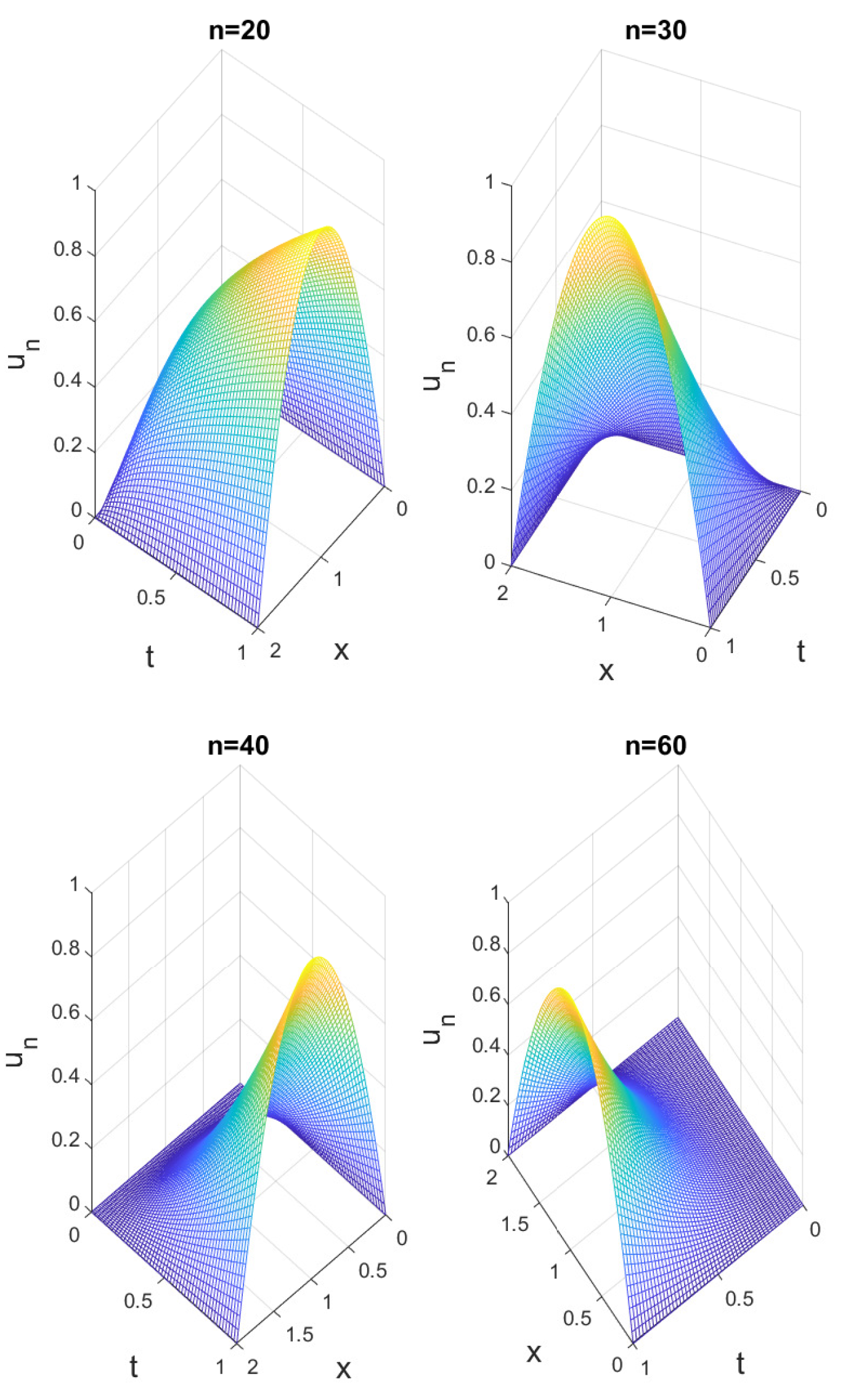
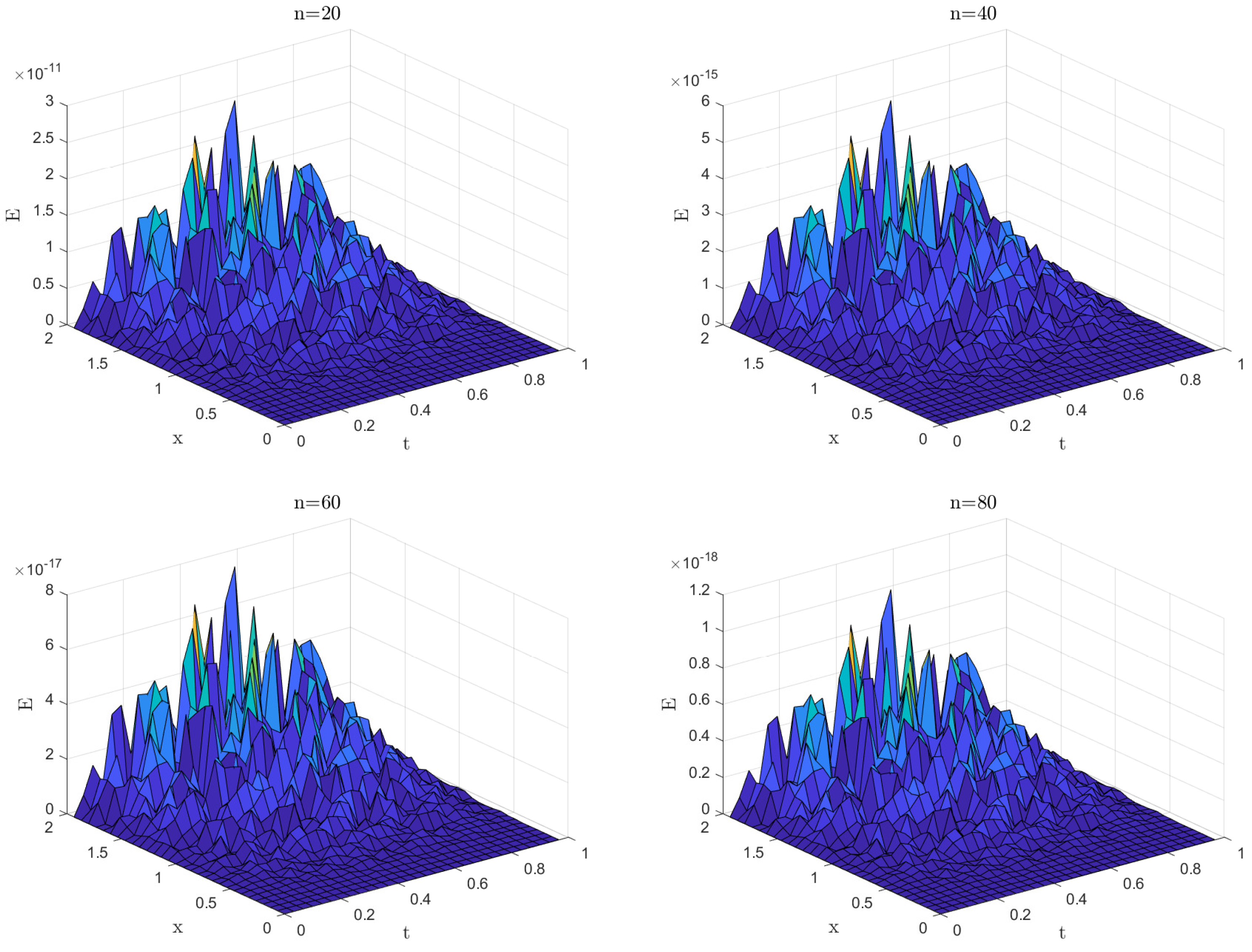
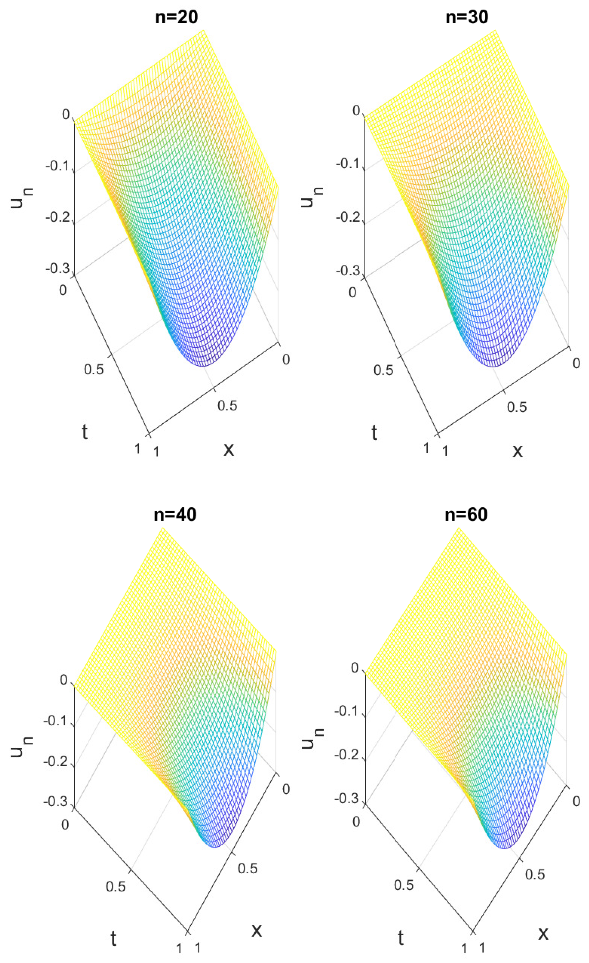
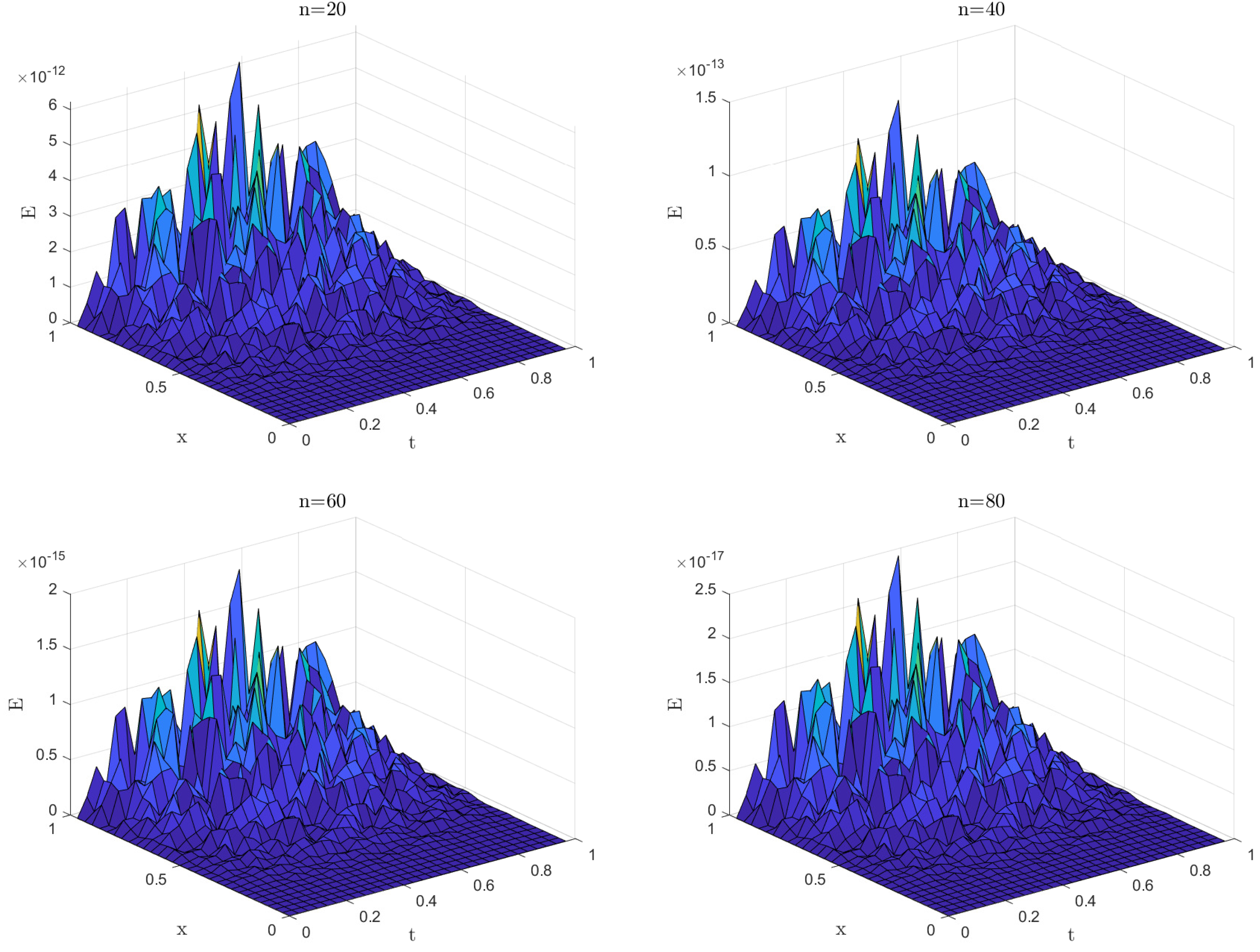
5. Numerical Simulation

To draw and present the proposed numerical method, we present some numerical examples. Here, the absolute error formula is given by

$$\mathrm{E}=|u-u_n|,$$

(42)

in which the function u shows the exact solution and $u_n$ shows the approximate solution.

Example 1.

Consider the following Korteweg–de Vries model:

$$\begin{array}{c}\hfill {\int }_0^1{\displaystyle \frac{\Gamma (8-\mu )}{6}}{\mathfrak{D}}_t^{\mu }ud\mu +3(u^2{)}_x+{\displaystyle \frac{{\partial }^{3}u}{\partial x^3}}=g,\end{array}$$

in which

$$\begin{array}{c}\hfill g(x,t)=(t^7-t^6)x{(1-x)}^2+6{(1-t^6)}^2(3x^5-10x^4+12x^3-6x^2+x)+6(1-t^6).\end{array}$$

The exact solution is $u=(1-t^6)x{(1-x)}^2$. We solved this problem by using the studied method for various values of $n=20,30,40$ with $\mathit{s}=40$.

Table 1. The absolute error for different values of n and $\mathbf{s}=40$ for Example 1.

$(\mathit{x},\mathit{t})$	$|\mathit{u}-{\mathit{u}}_{\mathit{n}}|$
	$n=20$	$n=30$	$n=40$
$(0.2,0.2)$	$1.3566\times {10}^{-12}$	$9.6722\times {10}^{-13}$	$4.5479\times {10}^{-14}$
$(0.4,0.4)$	$1.0849\times {10}^{-12}$	$1.0125\times {10}^{-12}$	$7.1512\times {10}^{-14}$
$(0.6,0.6)$	$3.5372\times {10}^{-12}$	$6.5661\times {10}^{-14}$	$4.2923\times {10}^{-14}$
$(0.8,0.8)$	$8.5690\times {10}^{-12}$	$1.6179\times {10}^{-13}$	$4.3111\times {10}^{-14}$
$(0.9,0.9)$	$1.0115\times {10}^{-11}$	$2.5824\times {10}^{-13}$	$4.5204\times {10}^{-14}$
$CPU$	$24.3$	$32.8$	$38.5$

represents the absolute error for the proposed numerical method for various values of n with $\mathit{s}=40$. Figure 1 represent the graphs of the numerical solutions for different values of n with $\mathit{s}=40$.

Example 2.

Consider

$$\begin{array}{cc}\hfill {\int }_0^1{\varrho }_{\mu }{\mathfrak{D}}_t^{\mu }u(x,t)d\mu & +u(x,t)u_x(x,t)+{\displaystyle \frac{1}{6}}{u}_{xxx}(x,t)=-2f_x(x,t)+{\displaystyle \frac{(t^2-t)x(2-x)}{lnt}}+t^4(2-x)(2-2x)\hfill \\ \hfill & +2\left({\displaystyle \frac{2}{3}}+(2t-2)e^{-t^2+2t-1}\right)sec{h}^2(x-e^{-t^2+2t-1})tanh(x-e^{-t^2+2t-1}),\hfill \\ \hfill u(x,0)& =0,\hfill \end{array}$$

(43)

in which

$$f(x,t)=-\left({\displaystyle \frac{2}{3}}+(2t-2)e^{-t^2+2t-1}\right)sec{h}^2(x-e^{-t^2+2t-1})$$

and ${\varrho }_{\mu }=\Gamma (3-\mu )$. For this problem, the analytical solution is $u=t^{2}x(2-x)$. Graphs of the approximate solutions for the problem are shown in Figure 2, and graphs of the absolute error function are displayed in Figure 3 for the values of n and $\mathit{s}=25$. From this figure, we see that when the value of n is increased, the absolute error is decreased.

Example 3.

Consider

$$\begin{array}{cc}\hfill {\int }_0^1{\varrho }_{\mu }{\mathfrak{D}}_t^{\mu }u(x,t)d\mu & +u{u}_x(x,t)+{\displaystyle \frac{1}{6}}{u}_{xxx}=-2f_x+{\displaystyle \frac{\sqrt{t}(t^2-t)x(x-1)}{lnt}}+t^5(2x-1)x(x-1)\hfill \\ \hfill & +2\left({\displaystyle \frac{2}{3}}+(2t-2)e^{-t^2+2t-1}\right)sech(x-e^{-t^2+2t-1})tanh(x-e^{-t^2+2t-1}),\hfill \\ \hfill u(x,0)& =0,\hfill \end{array}$$

(44)

in which

$$f(x,t)=-\left({\displaystyle \frac{2}{3}}+(2t-2)e^{-t^2+2t-1}\right)sech(x-e^{-t^2+2t-1})$$

and ${\varrho }_{\mu }={\displaystyle \frac{8}{15\pi \Gamma (\frac{7}{2}-\mu )}}$. For this problem, the analytical solution is $u(x,t)=t^{{\displaystyle \frac{5}{2}}}x(x-1)$. We solved this problem for different values of n using the numerical method. Graphs of the numerical results for different values of n are depicted in Figure 4. Figure 5 shows graphs of the absolute error function for the values of n and $\mathit{s}=25$. From this figure, we see that when the value of n is increased, the absolute error is decreased.

6. Conclusions

This study presents a numerical technique based on the shifted Legendre polynomials for obtaining the approximate solutions of Equation (1) under the stated conditions. Using this numerical method, an operational matrix is derived to solve the projected model. Also, convergence and error are investigated in this study. Some examples are displayed for the effectiveness of the numerical approach. Numerical results for all numerical examples are demonstrated in the form of graphs. From these graphs, we understand that the given numerical method is an efficient method with a high accuracy. The present research may help researchers to investigate nonlinear models with efficient tools and derive some simulating results, which may help capture more essential properties of the corresponding results.

References

1. Chen, Z.; Kosari, S.; Shafi, J.; Derakhshan, M.H. Stability Analysis Study of Time-Fractional Nonlinear Modified Kawahara Equation Based on the Homotopy Perturbation Sadik Transform. Fractal Fract. 2024, 8, 512. [Google Scholar] [CrossRef]
2. Hashemi, M.S.; Abbasbandy, S. A geometric approach for solving Troesch’s problem. Bull. Malays. Math. Sci. Soc. 2017, 40, 97–116. [Google Scholar] [CrossRef]
3. Inc, M.; Parto-Haghighi, M.; Akinlar, M.A.; Chu, Y.M. New numerical solutions of fractional-order Korteweg-de Vries equation. Results Phys. 2020, 19, 103326. [Google Scholar] [CrossRef]
4. Kosari, S.; Xu, P.; Shafi, J.; Derakhshan, M.H. An efficient hybrid numerical approach for solving two-dimensional fractional cable model involving time-fractional operator of distributed order with error analysis. Numer. Algorithms 2024, 17, 1–20. [Google Scholar] [CrossRef]
5. Pourbabaee, M.; Saadatmandi, A. A novel Legendre operational matrix for distributed order fractional differential equations. Appl. Math. Comput. 2019, 361, 215–231. [Google Scholar] [CrossRef]
6. David, V.D.; Nazari, M.; Barati, V.; Salah, F.; Abdul Aziz, Z. Approximate analytical solution for the forced Korteweg-de Vries equation. J. Appl. Math. 2013, 2013, 795818. [Google Scholar] [CrossRef]
7. Akylas, T.R. On the excitation of long nonlinear water waves by a moving pressure distribution. J. Fluid Mech. 1984, 141, 455–466. [Google Scholar] [CrossRef]
8. Jun-Xiao, Z.; Bo-Ling, G. Analytic solutions to forced KdV equation. Commun. Theor. Phys. 2009, 52, 279. [Google Scholar] [CrossRef]
9. Grimshaw, R.; Pelinovsky, E.; Tian, X. Interaction of a solitary wave with an external force. Phys. D Nonlinear Phenom. 1994, 77, 405–433. [Google Scholar] [CrossRef]
10. Pelinovsky, E.; Talipova, T.; Kurkin, A.; Kharif, C. Nonlinear mechanism of tsunami wave generation by atmospheric disturbances. Nat. Hazards Earth Syst. Sci. 2001, 1, 243–250. [Google Scholar] [CrossRef]
11. Derakhshan, M.H.; Rezaei, H.; Marasi, H.R. An efficient numerical method for the distributed-order time-fractional diffusion equation with the error analysis and stability properties. Math. Methods Appl. Sci. 2023, 214, 315–333. [Google Scholar] [CrossRef]
12. Liao, S.J.; Cheung, K.F. Homotopy analysis of nonlinear progressive waves in deep water. J. Eng. Math. 2003, 45, 105–116. [Google Scholar] [CrossRef]
13. Liao, S.J. An analytic approximate approach for free oscillations of self-excited systems. Int. J. -Non-Linear Mech. 2004, 39, 271–280. [Google Scholar] [CrossRef]
14. Liao, S.J. On the analytic solution of magnetohydrodynamic flows of non-Newtonian fluids over a stretching sheet. J. Fluid Mech. 2003, 488, 189–212. [Google Scholar] [CrossRef]
15. Grimshaw, R.H.; Maleewong, M. Transcritical flow over obstacles and holes: Forced Korteweg—De Vries framework. J. Fluid Mech. 2019, 881, 660–768. [Google Scholar] [CrossRef]
16. Hereman, W. Shallow water waves and solitary waves. arXiv 2013, arXiv:1308.5383. [Google Scholar]
17. Ali, R.; Saha, A.; Chatterjee, P. Analytical electron acoustic solitary wave solution for the forced KdV equation in superthermal plasmas. Phys. Plasmas 2017, 24, 122106. [Google Scholar] [CrossRef]
18. Mandi, L.; Mondal, K.K.; Chatterjee, P. Analytical solitary wave solution of the dust ion acoustic waves for the damped forced modified Korteweg-de Vries equation in q-nonextensive plasmas. Eur. Phys. J. Spec. Top. 2019, 228, 2753–2768. [Google Scholar] [CrossRef]
19. Ji, J.; Zhang, L.; Wang, L.; Wu, S.; Zhang, L. Variable coefficient KdV equation with time-dependent variable coefficient topographic forcing term and atmospheric blocking. Adv. Differ. Equ. 2019, 2019, 320. [Google Scholar] [CrossRef]
20. Kurulay, M.; Bayram, M. Approximate analytical solution for the fractional modified KdV by differential transform method. Commun. Nonlinear Sci. Numer. Simul. 2010, 15, 1777–1782. [Google Scholar] [CrossRef]
21. Ganji, D.D.; Nourollahi, M.; Rostamian, M. A comparison of variational iteration method with Adomian’s decomposition method in some highly nonlinear equations. Int. J. Sci. Technol. 2007, 2, 179–188. [Google Scholar]
22. Rawashdeh, M. Improved approximate solutions for nonlinear evolutions equations in mathematical physics using the reduced differential transform method. J. Appl. Math. Bioinform. 2013, 3, 1. [Google Scholar]
23. Yazid, N.M.; Tay, K.G.; Choy, Y.Y.; Sudin, A.M.; Tiong, W.K.; Ong, C.T. Numerical Solution of the Forced Korteweg-de Vries (fKDV) Equation. ARPN J. Eng. Appl. Sci. 2006, 11, 10757–10760. [Google Scholar]
24. Lee, S. Dynamics of trapped solitary waves for the forced KdV equation. Symmetry 2018, 10, 129. [Google Scholar] [CrossRef]
25. Taghipour, M.; Aminikhah, H. Numerical solution of distributed-order fractional Korteweg-de Vries equation via fractional Zigzag rising diagonal functions. Numer. Algorithms 2024, 96, 739–776. [Google Scholar] [CrossRef]
26. Balamurugan, S.; Vigneshwaran, S. Exact Solutions for a Compound KDV-Burgers Equation with Forcing Term. Int. J. Math. Trends Technol. 2018, 56, 320–330. [Google Scholar]
27. Hattam, L.L.; Clarke, S.R. Modulation theory for the steady forced KdV-Burgers equation and the construction of periodic solutions. Wave Motion 2015, 56, 67–84. [Google Scholar] [CrossRef]
28. Zergania, S.; Leec, J.H.; Aziza, Z.A.; Viswanathan, K.K. KDV and FKDV Model for the Run-up of Tsunamis via Lattice Boltzmann Method. Int. J. Appl. Eng. Res. 2017, 12, 14338–14347. [Google Scholar]
29. Saadatmi, A.; Khani, A.; Azizi, M.R. Numerical Calculation of Fractional Derivatives for the Sinc Functions via Legendre Polynomials. Math. Interdiscip. Res. 2019, 1, 71–86. [Google Scholar]
30. Hildebr, F.B. Introduction to Numerical Analysis; Courier Corporation: North Chelmsford, MA, USA, 1987. [Google Scholar]
31. Mashayekhi, S.; Ordokhani, Y.; Razzaghi, M. A hybrid functions approach for the Duffing equation. Phys. Scr. 2013, 88, 025002. [Google Scholar] [CrossRef]
Figure 1. Graph of numerical results for Example 1 with different kinds of n with s = 25 .
Fractalfract 08 00630 g001
Figure 2. Graph of numerical solutions when s = 25 for Example 2 with different kinds of n.
Fractalfract 08 00630 g002
Figure 3. A diagram of the absolute errors when s = 40 for Example 2 with different values of n.
Fractalfract 08 00630 g003
Figure 4. Graph of numerical results for Example 3 with different kinds of n with s = 25 .
Fractalfract 08 00630 g004
Figure 5. Absolute errors of Example 3 for different values of n with s = 40 .
Fractalfract 08 00630 g005