Article

Deep-Learning Estimators for the Hurst Exponent of Two-Dimensional Fractional Brownian Motion

by
Yen-Ching Chang
1,2
1
Department of Medical Informatics, Chung Shan Medical University, Taichung 40201, Taiwan
2
Department of Medical Imaging, Chung Shan Medical University Hospital, Taichung 40201, Taiwan
Fractal Fract. 2024, 8(1), 50; https://doi.org/10.3390/fractalfract8010050
Submission received: 20 December 2023 / Revised: 31 December 2023 / Accepted: 10 January 2024 / Published: 12 January 2024
(This article belongs to the Section Numerical and Computational Methods)

Abstract

:
The fractal dimension (D) is a very useful indicator for recognizing images. The fractal dimension increases as the pattern of an image becomes rougher. Therefore, images are frequently described as certain models of fractal geometry. Among the models, two-dimensional fractional Brownian motion (2D FBM) is commonly used because it has specific physical meaning and only contains the finite-valued parameter (a real value from 0 to 1) of the Hurst exponent (H). More usefully, H and D possess the relation of D = 3 − H. The accuracy of the maximum likelihood estimator (MLE) is the best among estimators, but its efficiency is appreciably low. Lately, an efficient MLE for the Hurst exponent was produced to greatly improve its efficiency, but it still incurs much higher computational costs. Therefore, in the paper, we put forward a deep-learning estimator through classification models. The trained deep-learning models for images of 2D FBM not only incur smaller computational costs but also provide smaller mean-squared errors than the efficient MLE, except for size 32 × 32 × 1. In particular, the computational times of the efficient MLE are up to 129, 3090, and 156248 times those of our proposed simple model for sizes 32 × 32 × 1, 64 × 64 × 1, and 128 × 128 × 1.

1. Introduction

When describing particular images (or surfaces) and signals, the fractal structure often plays a very effective role. For example, Huang and Lee [1] used fractal analysis to classify pathological prostate images; Lin et al. [2] also adopted fractal analysis to classify solitary pulmonary nodules; He and Liu [3] screened dry coal online through fractal analysis and image processing; Yakovlev et al. [4] also used fractal analysis to evaluate changes in a modified cement composite; Guo et al. [5] characterized and classified tumor lesions of digital mammograms through fractal texture analysis; Crescenzo et al. [6] adopted FBM to predict temperature fluctuation; Paun et al. [7] used fractal analysis to evaluate micro fractographies; and Hu et al. [8] combined FBM and particle swarm optimization to propose a stock prediction model.
It is common for signals and images to use the fractal dimension (FD) to explain and recognize irregular structures; the smaller the FD, the smoother the signal/image. Accordingly, the intensities in the pathological tissues of medical images are usually viewed as fractal images. Therefore, the FD is a very suitable indicator for differentiating between these two different tissues.
Among the models for describing irregular images, two-dimensional fractional Brownian motion (2D FBM) [9,10] is an excellent choice because it can explain the characteristics of images in the sense of physical activity. In contrast, its corresponding two-dimensional fractional Gaussian noise (2D FGN) is also another excellent selection, in that it can describe much rougher patterns. These two models are not only suitable for describing many medical images; they are also appropriate for characterizing many natural scenes [11,12,13]. For traditional estimators, these two models must be separately considered and applied. For deep-learning estimators, they can be trained together and further explained. It is a promising avenue to consider images of 2D FBM and 2D FGN for deep-learning models.
Both 2D FBM and 2D FGN only contain the Hurst exponent (H)—a real value between 0 and 1—which can easily distinguish between images of the Hurst exponent with various realizations; the value of H and FD (D) possesses the relation of D = 3 − H [10]. Since the values of the Hurst exponent are in the range from 0 to 1, it is very likely to act as an important feature. In particular, its range is considerably appropriate to serve as the domain of images. When all sub-images of an original image are transformed into estimates of the Hurst exponent, these estimates (0–1) can be saved as a feature/characteristic image/map for another input source image. When machine-learning or deep-learning models are run on certain images, we can supply this characteristic image for another input to improve the overall classification rate through two inputs (the original source images and their corresponding transformed characteristic images) and/or two model streams.
Typically, based on the Hurst exponent, its effectiveness is related to the accuracy of estimation; that is, the higher the accuracy of estimation, the better the classification rate. Therefore, the better the estimators, the higher the benefits of the Hurst exponent. Over the past decades, some estimators have been calculated via the fractal model [14], some through the fractal feature [15], fractal approach [16], the box-counting method [17,18,19,20,21,22], and the blanket [23]. No matter which method is chosen, we often need to balance between the accuracy and efficiency of estimators. Nevertheless, optimal accuracy is always welcome by users, except when its computational cost is unbearable.
As we know, the accuracy of the maximum likelihood estimator (MLE) is the best among estimators, but its efficiency is appreciably low and even prohibitive. In order to raise its value, Chang [24] recently proposed two versions of MLE for the 2D FBM and 2D FGN: one is called an iterative MLE, and the other is called an efficient MLE. The efficient MLE is much better in terms of efficiency than the iterative MLE, and the iterative MLE is much better in terms of efficiency than the standard MLE or simply MLE. Currently, it is—without a doubt—our best choice to use the efficient MLE to estimate the Hurst exponent.
Before the era of machine learning, we had often used these estimates to distinguish between various tissues or images; generally, this approach was effective for significant differences between images. At the moment, we—in the era of machine learning—can also classify images using these estimates as another feature; this machine-learning approach is typically better than the conventional approach, especially for small differences between images.
As deep learning becomes more and more advanced and mature in algorithms and technologies, in the upcoming future, we are going to use the corresponding characteristic images of all the original images as extra input and then design two inputs and/or two model streams to distinguish between different images. Compared to a single image input, two or more image inputs will intuitively improve the overall classification rate through deep-learning models. It can be expected that this deep-learning approach will be much better than the machine-learning approach, especially for tiny differences between images.
In the future, we will develop multiple inputs and/or diverse model streams to distinguish between different images. Their inputs will contain other characteristic images or maps, such as entropy or spectrum images.
In the past, when images were modeled as 2D FBM, we estimated their Hurst exponents via estimators and then viewed these estimates as an indicator. It is well known that any estimator will contain errors. In addition, the weakness of the best estimator is usually its higher computational cost, even when the error has been much reduced by an efficient MLE [24].
Over the past decade, deep-learning models have flourished. As rich and diverse pre-trained models are developed, a feasible and even effective idea may be that estimates may be indirectly computed from deep-learning models, not directly from the estimators. This approach—estimating the Hurst exponent through deep-learning models—can be regarded as an indirect estimator, but the traditional estimator, such as the MLE, can be regarded as a direct estimator. For convenience, we designate these approaches using deep-learning models as deep-learning estimators. It turns out that deep-learning estimators outperform traditional estimators in terms of mean-squared errors and computational costs.
Since a rich resource of pre-trained deep-learning models was available, which were trained on a million images from the ImageNet database [25] to classify 1000 object categories, in the paper, we adopt deep-learning models for classification—not regression—to classify the Hurst exponent and then convert these classes to the corresponding values of the Hurst exponent. In the future, we will further modify these pre-trained models for classification to qualified pre-trained models for regression.
In a previous pilot study [26], we found that a simple deep-learning model and two pre-trained models—AlexNet and GoogleNet—with and without augmentation outperformed the MLE in terms of mean-squared errors (MSEs) in fractional Brownian images (FBIs—gray-level images saved from 2D FBM) with a size 32 × 32 × 1 under two equally spaced resolutions (11 and 21 classes). For each Hurst exponent, we generated 1000 FBIs. In order to fairly compare the MSEs between the MLE and three deep-learning models, five-fold cross-validation was adopted with the stochastic gradient descent with momentum (sgdm) solver.
At that time, the MSEs for deep-learning models were measured by converting the classified classes to the corresponding MSEs. Therefore, if the classified class is correct, its MSE is zero. The measurement seems to be reasonable, but it is not practical for real-world images, in that we do not know how to precisely segment the Hurst exponent in advance. Therefore, in the paper, we additionally generate a finer resolution of 32 classes to train the models and then use these models trained on 32 classes to classify 11 classes of images and then convert the classified classes to their corresponding MSEs. In this case, there are no absolutely correct classes, and hence, any class will result in an error. Based on the principle, a relatively fair comparison will be conducted.
On the surface, the finer the resolution, the higher the advantage of the deep-learning models. However, the finer resolution will give rise to complexity in training deep-learning models. Therefore, this approach can be used to test the power of deep-learning models.
For a fair comparison among deep-learning models, in the previous experiments, we generated 1000 FBIs through the same seeds (1–1000) from a pseudo-random-number generator. The set from seed 1 to 1000 is called Set 1. Using five-fold cross-validation, this approach seems to be reasonable and reliable because none of the validation images was involved in the training set. In order to understand whether deep-learning models will learn and memorize the hidden realizations from a pseudo-random-number generator, we will additionally generate another set of images from other seeds (1001–2000). The set from seed 1001 to 2000 is called Set 2.
In our study, three main issues will be discussed. The first issue is whether the deep-learning models trained on 32 classes from Set 1 are better in the classification rates and MSEs than those trained on 11 and 21 classes from the same seeds (Set 1) and whether the deep-learning models trained on 21 classes from Set 1 are also better in the classification rates and MSEs than those trained on 11 classes from the same seeds (Set 1). If so, these trained deep-learning models are qualified for estimating the Hurst exponent of FBIs. The evaluation approach of the experiment is called within-set evaluation; that is, deep-learning models trained on a large part of one set are evaluated on a small part of the same set through cross-validation. For five-fold cross-validation, the training set is 80% of one set, and the validation set is 20% of the same set.
For the second issue, we will perform two experiments: one involves Set 2 with 11 classes being evaluated by deep-learning models trained on Set 1 with 11 classes, and the other involves Set 1 with 11 classes being evaluated through five-fold cross-validation by deep-learning models trained on Set 1 with 11 classes. The evaluation approach of the former is called between-set evaluation; that is, deep-learning models trained on one set are evaluated on another set. The latter approach, as before, is within-set evaluation. If two evaluation approaches will give similar results, the deep-learning models for FBIs will possess an extremely high generalization ability. These models are robust against various realizations, and hence, they are extremely suitable for indirectly estimating the Hurst exponent or its corresponding fractal dimension. Otherwise, deep-learning models may learn the hidden realizations through different appearances from different Hurst exponents. The phenomenon suggests that the current deep-learning models possess high learning power.
As we know, any estimation must contain an error, but the MSEs of correctly classified classes are assigned zeros in the previous experiments; therefore, the operation is not fair for a comparison with the MLE. Therefore, addressing the third issue, we also want to know whether Set 2 with 11 classes evaluated by deep-learning models trained on Set 1 with 32 classes performs better in the MSEs and computational costs than the efficient MLE. If true, these models for FBIs are suitable for indirectly estimating the Hurst exponent. In the experiment, we use between-set evaluation, and no so-called correct classes occur; hence, the comparison is a very fair mechanism.
Therefore, in the paper, three resolutions—11, 21, and 32 equally spaced Hurst exponents—will be taken into consideration. For each resolution, we first estimate the Hurst exponents of fractional Brownian surfaces (FBSs—the numerical data of 2D FBM) and FBIs via the efficient MLE for comparison. Based on the same FBIs, we propose a simple deep-learning model and choose five pre-trained deep-learning models to classify and then convert the classified classes to the corresponding Hurst exponents. Likewise, their classification results and MSEs will be provided for further comparison.
Section 2 in the paper introduces some related materials and methods. Section 3 describes our experiments and provides wide results. A detailed discussion is presented in Section 4. Section 5 provides some possible applications in the future. Finally, Section 6 summarizes the results of the paper and presents some future works.

2. Materials and Methods

In brief, we will describe some materials and deep-learning models in this section. The primary materials include the non-stationary process of 2D FBM, its corresponding stationary increment process of 2D FGN, and an efficient MLE for the Hurst exponent: a traditional MLE run in an efficient way. In the end, the deep-learning models consist of our proposed model and five pre-trained models: GoogleNet, Xception, ResNet18, MobileNetV2, and SqueezeNet.

2.1. Two-Dimensional Fractional Brownian Motion

Falconer [10] used an index-H Brownian function to name the non-stationary process of 2D FBM, whereas Hoefer et al. [27] used an isotropic 2D FBM to name the process and an isotropic two-dimensional discrete FBM to name its corresponding discrete version. However, Balghonaim and Keller [28] used a two-variable FBM to name the process and a two-variable discrete FBS to name its corresponding discrete version. In the paper, we simply use 2D FBM to name the process.
Assuming an image (numerical data, not gray-level values or real numbers from gray-level values) of FBI with size M × N is denoted as follows:
I B = B 0 , 0 B 0 , 1 B 0 , N 1 B 1 , 0 B 1 , 1 B 1 , N 1 B M 1 , 0 B M 1 , 1 B M 1 , N 1
Taking out two points or coordinates B x 1 , y 1 and B x 2 , y 2 from the image of 2D FBM, we obtain their autocorrelation function (ACF) as follows:
r B B x 1 y 1 , x 2 y 2 = E B x 1 , y 1 B x 2 , y 2 = σ 2 2 x 1 y 1 2 H + x 2 y 2 2 H x 1 x 2 y 1 y 2 2 H
where E stands for the expectation operator; σ 2 is the variance in the process; is the Euclidean norm; H is the only parameter concerned, called the Hurst exponent. It is obvious that the ACF is directly calculated from the distance between two coordinates and two distances from the origin.
To estimate the Hurst exponent, the ACFs must be stationary—not non-stationary. There exist two feasible approaches for stationary ACFs. Hoefer et al. [27] put forward the first approach, simply called the first 2D FGN, by using the second increment process of 2D FBM. They also called the resultant process two-dimensional Gaussian noise (FGN2) [29]. Balghonaim and Keller [28] put forward the second approach, simply called the second 2D FGN, by using the first increment process on each row or column of 2D FBM.
Chang [24] has given a detailed description of these two 2D FGN. When his proposed efficient MLE was run on the second 2D FGN, the mean-squared errors (MSEs) were smaller than those on the first 2D FGN. Compared to the second 2D FGN, the first 2D FGN possesses more physical meanings because real images are usually present in the appearances of the first 2D FGN—seldom in the patterns of the second 2D FGN.
Therefore, we will adopt the first 2D FGN—not the second 2D FGN—to generate its probability density function (PDF) and then estimate the Hurst exponent through the efficient MLE. For the first 2D FGN, we first represent the data of 2D FBM as an image of 2D FBM, I B , which is a column vector with size M N × 1 , as follows:
B T = B 0 T B 1 T B M 1 T
where
B k T = B k , 0     B k , 1         B k , N 1 ,   k = 0 , 1 , , M 1 .
Based on the column vector, we can easily obtain its non-stationary covariance matrix from the following equation:
R B B = E B B T .
Next, we calculate the first 2D FGN from the second increment process [27] of 2D FBM, as follows:
X i , j = B i , j B i , j 1 B i 1 , j + B i 1 , j 1 , i = 1 , 2 , , M 1 ;   j = 1 , 2 , , N 1 .
Similar to the notation of the image of 2D FBM, we also represent this image of 2D FGN as a column vector with size N 1 × 1 , N 1 = M 1 N 1 :
X T = X 1 T X 2 T X M 1 T
where
X k T = X k , 1     X k , 2         X k , N 1 ,   k = 1 , 2 , , M 1 .
The vector, X T , can be regarded as a vector time series. Accordingly, its covariance is composed of a special structure, called a Toeplitz-block Toeplitz matrix, or a symmetric-block symmetric matrix, as follows:
R = R H , σ 2 = E X X T = R 0 R 1 R M 2 R 1 R 0 R M 3 R M 2 R M 3 R 0 ,
where
R k = R i , j = E X i X j T = F k , 0 F k , 1 F k , N 2 F k , 1 F k , 0 F k , N 3 F k , N 2 F k , N 3 F k , 0 ,
k = i j ,   i , j = 1 , 2 , , M 1 ,
where
F k , l = E X i 1 , j 1 X i 2 , j 2 = σ 2 2 f k , l ,
k = i 1 i 2 ,   l = j 1 j 2 ;   i 1 , i 2 = 1 , 2 , , M 1 ;   j 1 , j 2 = 1 , 2 , , N 1 ,
where
f k , l = 2 k 1 2 + l 2 H + 2 k 2 + l 1 2 H + 2 k 2 + l + 1 2 H + 2 k + 1 2 + l 2 H
k 1 2 + l 1 2 H k 1 2 + l + 1 2 H k + 1 2 + l 1 2 H k + 1 2 + l + 1 2 H 4 k 2 + l 2 H .
Obviously, all ACFs are directly connected with the relative distances—not absolute distances—between two coordinates; hence, the first 2D FGN is stationary, or the vector X T is a stationary vector time series. Accordingly, we can estimate the Hurst exponent through the MLE based on the PDF of this 2D FGN.

2.2. The Maximum Likelihood Estimator for 2D FBM

Through this 2D FGN, its corresponding PDF will be generated. Based on the PDF, two cases will be considered: one with the known variance, the other with the unknown variance. Without estimating the extra variance, the known variance case is theoretically better in terms of accuracy than the unknown variance case. In the paper, we only consider the unknown variance case, in that it is the most common case in the real world. Therefore, the PDF can be described in the following equation:
p X ; H , σ 2 = 1 2 π N 1 / 2 R 1 / 2 exp 1 2 X T R 1 X = 1 2 π N 1 / 2 σ 2 R ¯ 1 / 2 exp 1 2 σ 2 X T R ¯ 1 X ,
where
R = σ 2 R ¯ .
The above PDF consists of two parameters to be estimated by the efficient MLE. One is the unknown variance (an explicit parameter), and the other is the Hurst exponent (an implicit parameter). To estimate the explicit unknown variance, we first take the logarithm of the PDF, then maximize the log-likelihood function log p X ; H , σ 2 with respect to σ 2 , and finally obtain
log p X ; H , σ ^ 2 = N 1 2 log 2 π N 1 2 log σ ^ 2 1 2 log R ¯ N 1 2 ,
where
σ ^ 2 = 1 N 1 X T R ¯ 1 X .
Without affecting further estimation of the implicit parameter, the Hurst exponent—two constants and the common coefficient 0.5—is omitted, and then, we obtain a compact form in the following equation:
max H log p X ; H , σ ^ 2 = max H N 1 log 1 N 1 X T R ¯ 1 X log R ¯ .
From the elements of R ¯ , we know that the log-likelihood function only includes the parameter of the Hurst exponent, but in an implicit and inseparable way. Accordingly, it is not possible to directly maximize the log-likelihood function with respect to the implicit Hurst exponent. Instead, in the paper, we adopt the golden section search [30,31] to search for the best estimate.
Different from the traditional or original MLE for estimating the Hurst exponent, Chang [24] further proposed two quicker versions of the MLE: an iterative MLE and an efficient MLE. Both quicker MLEs have the same accuracies as the original MLE but different degrees of efficiency from the original MLE. The efficient MLE is faster than the iterative MLE, and hence, in the paper, we adopt the efficient MLE for comparison.

2.3. Deep-Learning Models

Szymak et al. [32] used pre-trained deep-learning models to classify objects in underwater videos. Maeda-Gutiérrez et al. [33] fine-tuned pre-trained deep-learning models to recognize the diseases of tomato plant. In the paper, we choose five pre-trained models—namely GoogleNet, Xception, ResNet18, MobileNetV2, and SqueezeNet—to classify 2D FBM.
GoogleNet [34] is a convolutional neural network, which is 22 layers deep [35], with 144 layers in total. It is also a pre-trained model, trained on more than a million images from the ImageNet database or Places365 [36]. The model trained on ImageNet [25] can classify images into 1000 object categories. Similar to the network trained on ImageNet, the model trained on Places365 can classify images into 365 different place categories. The model has an image input size of 224 × 224.
Xception [37] is a 71-layer-deep convolutional neural network [35], with 170 layers in total. It is a pre-trained model, trained on more than a million images from the ImageNet database. As with GoogleNet, the pre-trained model can also classify images into 1000 object categories. Therefore, the model learns rich feature structures. The model has an image input size of 299 × 299.
ResNet18 [38] is an 18-layer-deep convolutional neural network [35], with 71 layers in total. As with Xception, it is also a pre-trained model. Likewise, the pre-trained model can recognize 1000 object categories. The model has an image input size of 224 × 224, same as GoogleNet.
MobileNetV2 [39] is a 53-layer-deep convolutional neural network [35], with 154 layers in total. As with ResNet-18, it is also a pre-trained model. The pre-trained model can similarly classify images into 1000 object categories. The model has an image input size of 224 × 224, same as GoogleNet and ResNet18.
SqueezeNet [40] is an 18-layer-deep convolutional neural network [35], with 68 layers in total. As with MobileNetV2, it is also a pre-trained model, trained on more than a million images from the ImageNet database. The pre-trained model can also recognize 1000 object categories. The model has an image input size of 227 × 227.
Among these five pre-trained models, Xception (71 layers deep, 170 layers in total) is the layer-deepest and has the highest number of layers. The second layer-deepest and with the second highest number of layers is MobileNetV2 (53 layers deep, 154 layers in total). Based on layer depth and the number of layers, Xception has the most complex structure, followed by MobileNetV2 and GoogleNet (22 layers deep, 144 layers in total). The layer depth and number of layers of ResNet18 (18 layers deep, 71 layers in total) are similar to those of SqueezeNet (18 layers deep, 68 layers in total).
The number of layers of MobileNetV2 is only 10 larger than that of GoogleNet, but the layer depth of MobileNetV2 is 31 higher than GoogleNet. As a result, the structure of MobileNetV2 is lanky (high and thin), whereas that of GoogleNet is squat (short and fat).
Except for the five pre-trained deep-learning models, in the paper, we are going to propose a simple deep-learning model with 25 layers in order to understand whether a simple model has the ability to classify images of 2D FBM. For effective classification, it is necessary for machine-learning models to manually select features ahead of time by users, but it is not necessary for deep-learning models. Compared to machine-learning models, one of the main advantages of deep-learning models is that they can automatically capture as many patterns as possible depending on their structures and powers and then integrate them through intricate algorithms or mechanisms into significant features.

3. Experimental Results

In the paper, we will evaluate the performance of the efficient MLE and deep-learning models on two resolutions: 0.0909 (1/11) and 0.0476 (1/21). For the efficient MLE, we will estimate two kinds of data: fractional Brownian surfaces (FBSs) (true data) and fractional Brownian images (FBIs), which are obtained from FBSs saved as gray-level images, thereby losing some finer details, especially for larger image sizes. In addition, we will also calculate the corresponding MSEs for comparison. For deep-learning models—including our proposed deep-learning model with 25 layers, GoogleNet, Xception, ResNet18, MobileNetV2, and SqueezeNet—we will first classify these FBIs and then compute the corresponding Hurst exponents according to the formula of Hurst exponents versus classes and finally compute their MSEs.

3.1. Experimental Settings

To investigate the effectiveness, two kinds of classes—11 Hurst exponents and 21 Hurst exponents—will be considered. For 11 classes, the Hurst exponents are H = 1/22, 3/22, …, and 21/22; for 21 classes, the Hurst exponents are H = 1/42, 3/42, …, and 41/42. Hence, the resolution of 11 classes is 0.0909 (1/11), and the resolution of 21 classes is 0.0476 (1/21).
Similar to Hoefer et al. [28], we generated as our dataset 1000 realizations (seed 1–1000, called Set 1) or observations of 2D FBM for each Hurst exponent or class, and each realization had five sizes: 8 × 8 × 1, 16 × 16 × 1, 32 × 32 × 1, 64 × 64 × 1, and 128 × 128 × 1. They were saved as images (called FBIs) as well as numerical data (called FBSs for the efficient MLE) for comparison. In addition, we also generated another 1000 realizations (seed 1001–2000, called Set 2) as our comparison set. The realizations and appearances/images from Set 2 will not be completely seen by deep-learning models trained on Set 1. Although the appearances or images from Set 1 will not be completely seen through five-fold cross-validation by deep-learning models trained on Set 1, the realizations from Set 1 will be partially seen through five-fold cross-validation by deep-learning models trained on Set 1.
When generating each 2D FBM, we followed the following procedure. First, we calculated the covariance matrix according to Equation (4). Second, we decomposed the covariance matrix using Cholesky factorization to obtain its lower triangular. Third, we produced a realization of standard white Gaussian noise. Finally, we multiplied the lower triangular and the white noise to generate a realization of 2D FBM. Hence, for each size with 1000 observations, we produced 11,000 images and surfaces in total for 11 Hurst exponents and 21,000 images and surfaces in total for 21 Hurst exponents. It is worth mentioning again that FBIs are close to FBSs, with some information or finer details being lost.
For a fairer performance comparison of the MLE and deep-learning models, another 32 equally spaced classes or Hurst exponents were generated from Set 1 to train deep-learning models as our comparison models; that is, FBIs of 11 classes from Set 2 were evaluated on three models (among six models) trained on 32 classes from Set 1.
This approach has two purposes. As we know, any estimator will essentially cause errors to occur. The first purpose is to avoid the possibility of zero error. However, if we indirectly obtain the corresponding MSEs according to the formula of MSEs versus classes, then all correctly classified classes will be zero errors. This is not fair for comparison with the MLE.
When FBIs of 11 classes are evaluated on the trained models of 32 classes, no class will result in zero error. For example, the first class of 11 Hurst exponents is 1/22; if the trained models are sufficiently good, then they are classified possibly in the first few classes of 32 Hurst exponents: 1/64 (squared error of 8.8980 × 10−04), 3/63 (squared error of 2.0177 × 10−06), or 5/64 (squared error of 0.0011). The best estimate lies in the second class; its squared error is 2.0177 × 10−06, not zero.
The second purpose is that we would like to know whether the hidden realizations can be learned through five-fold cross-validation by deep-learning models. As we know, under five-fold cross-validation, the deep-learning models will not see these validated or tested images, and hence, the operation is theoretically considerably fair. However, during training, the models have partially seen their hidden realizations through five-fold cross-validation.
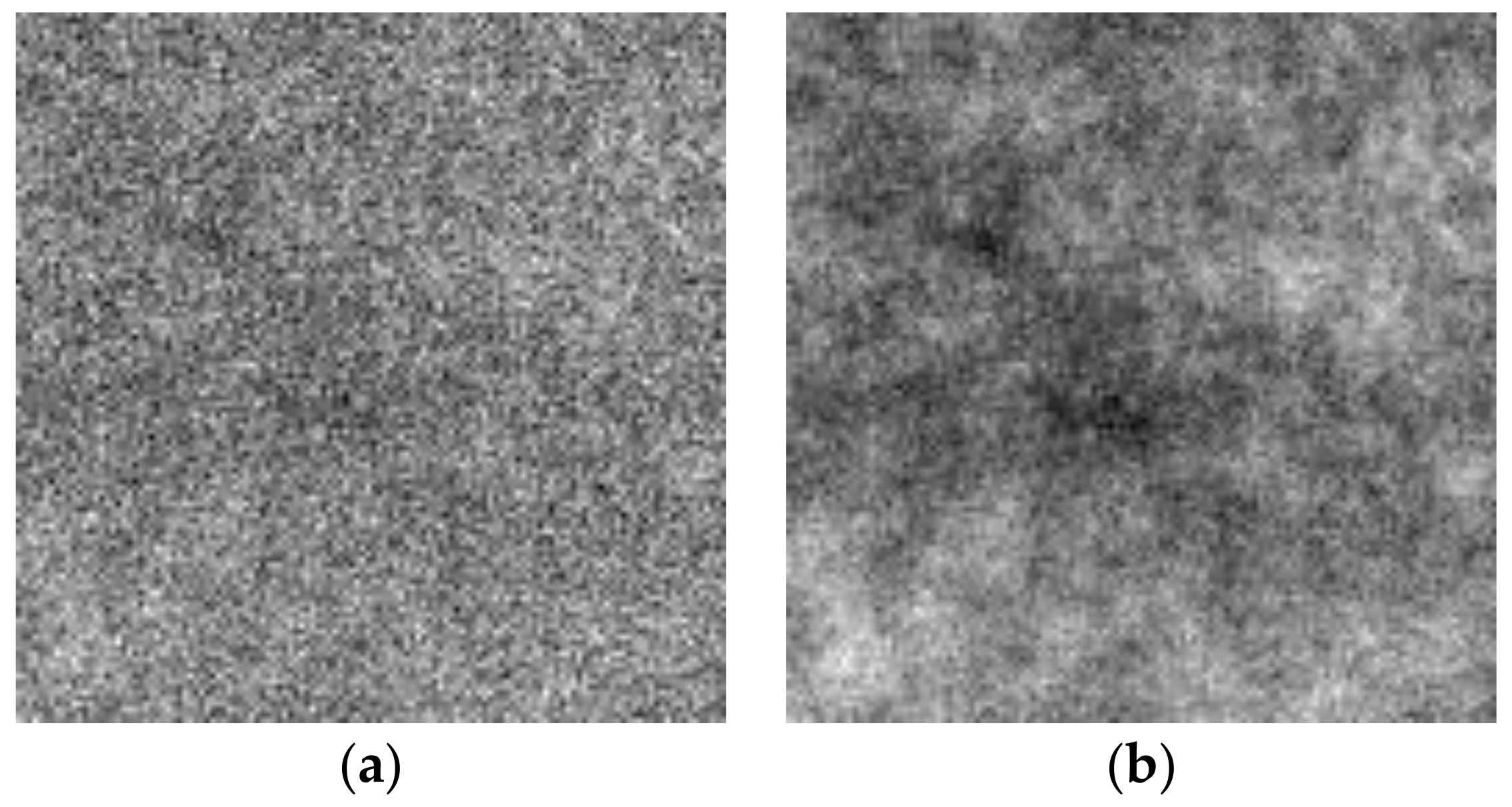
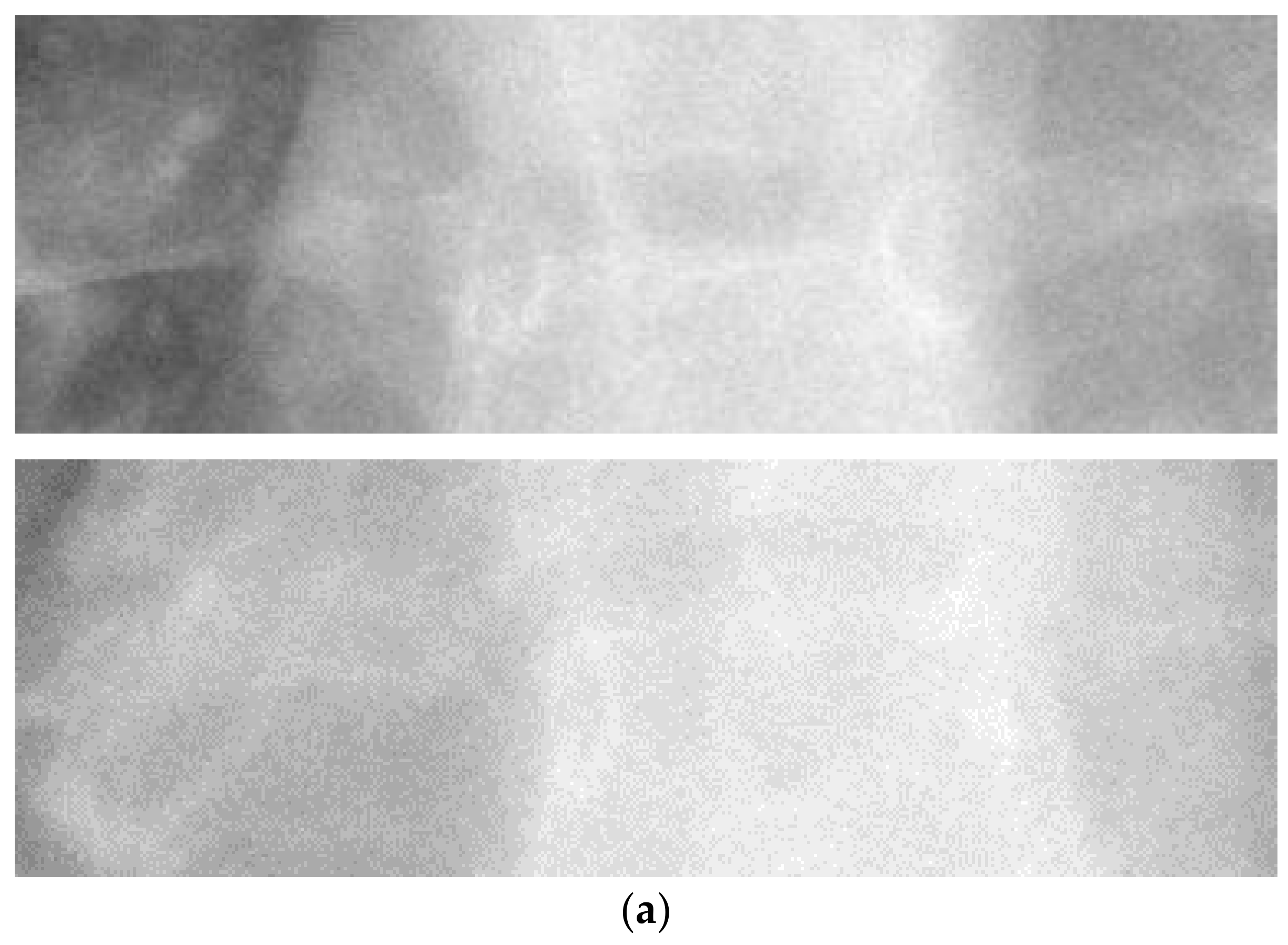
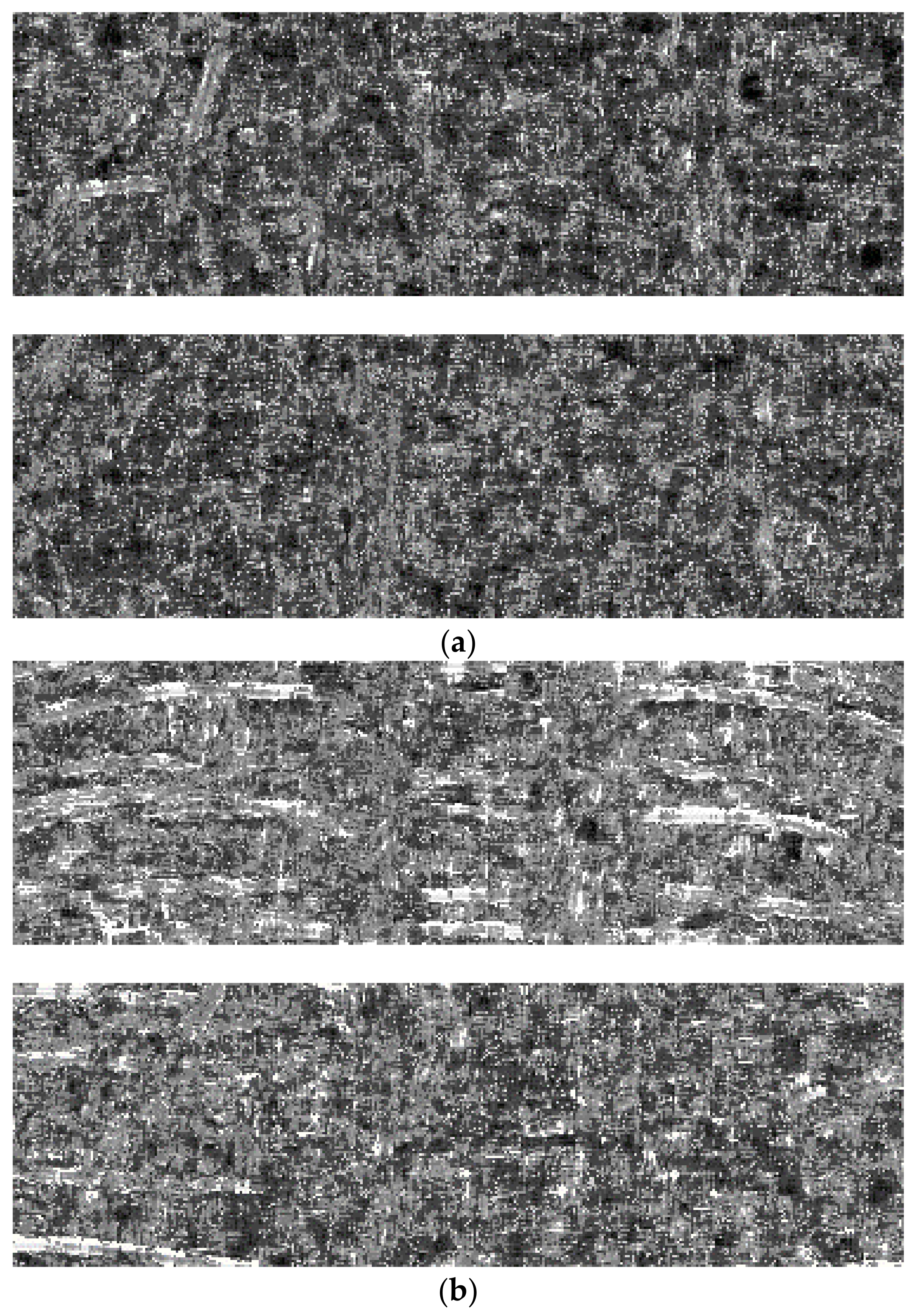
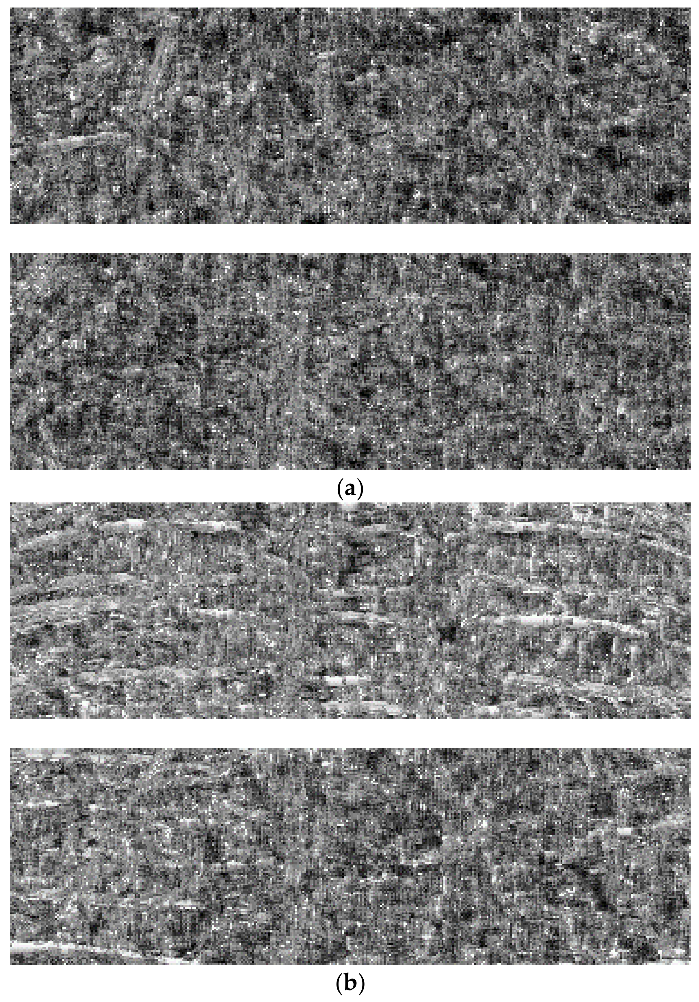
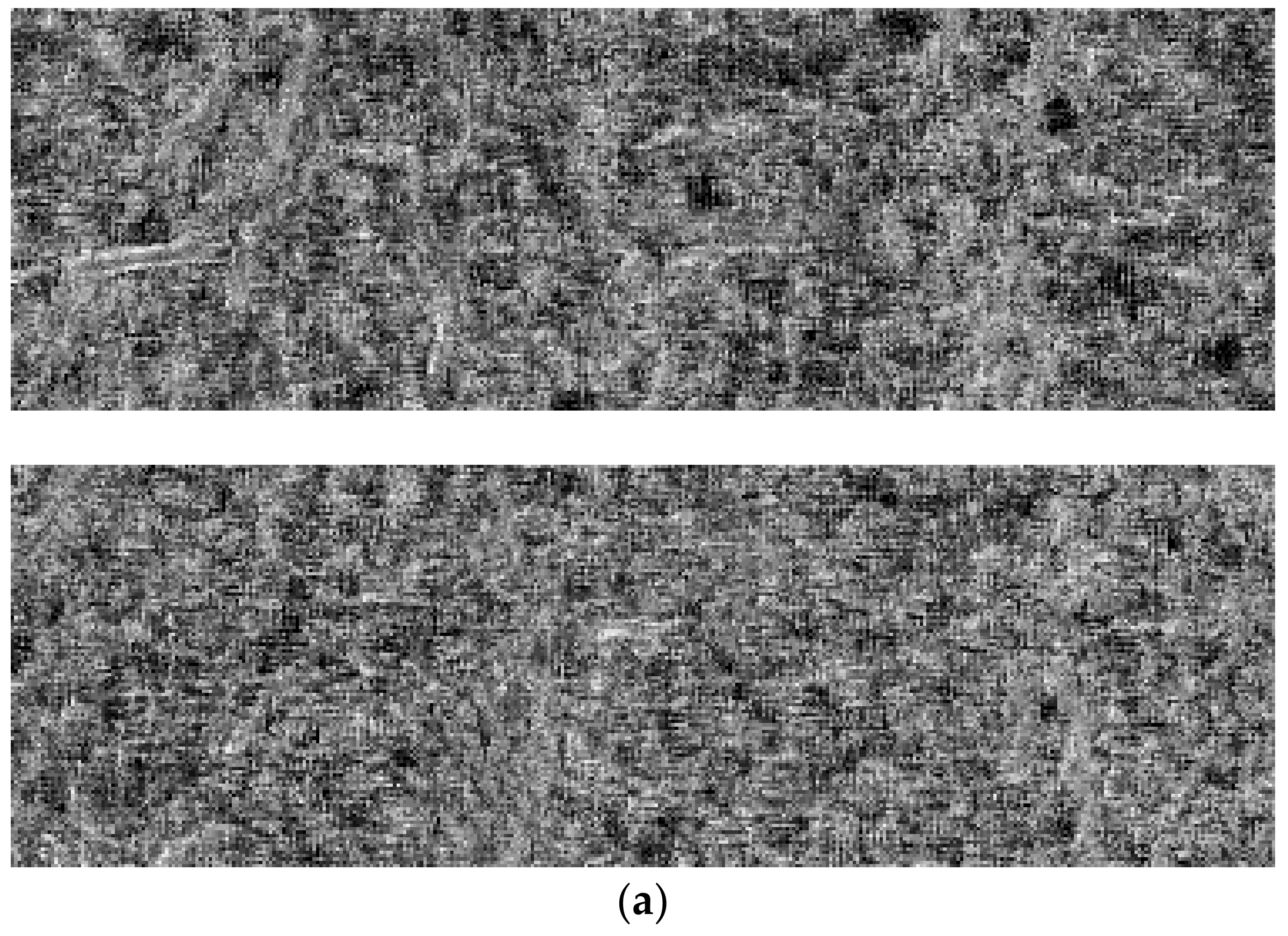
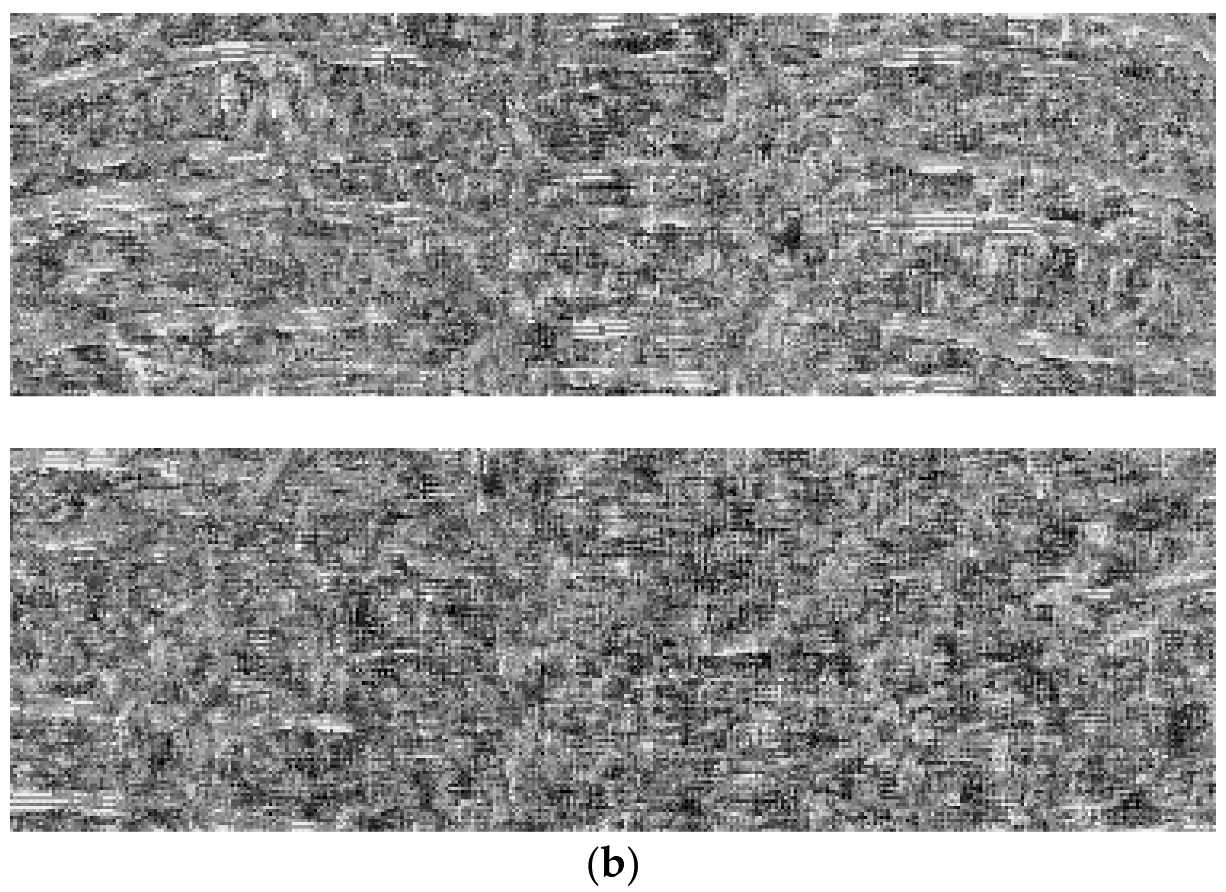
To illustrate some possible images or appearances of different Hurst exponents, Figure 1 shows two FBIs of H = 1/64 and H = 9/64 with size 128 × 128 × 1; 
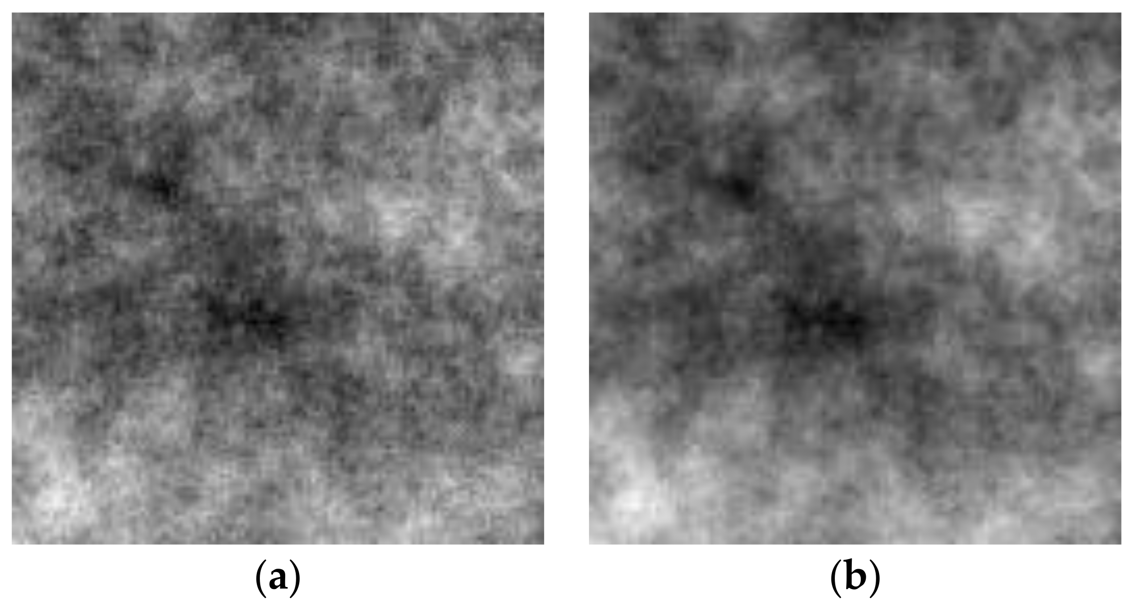
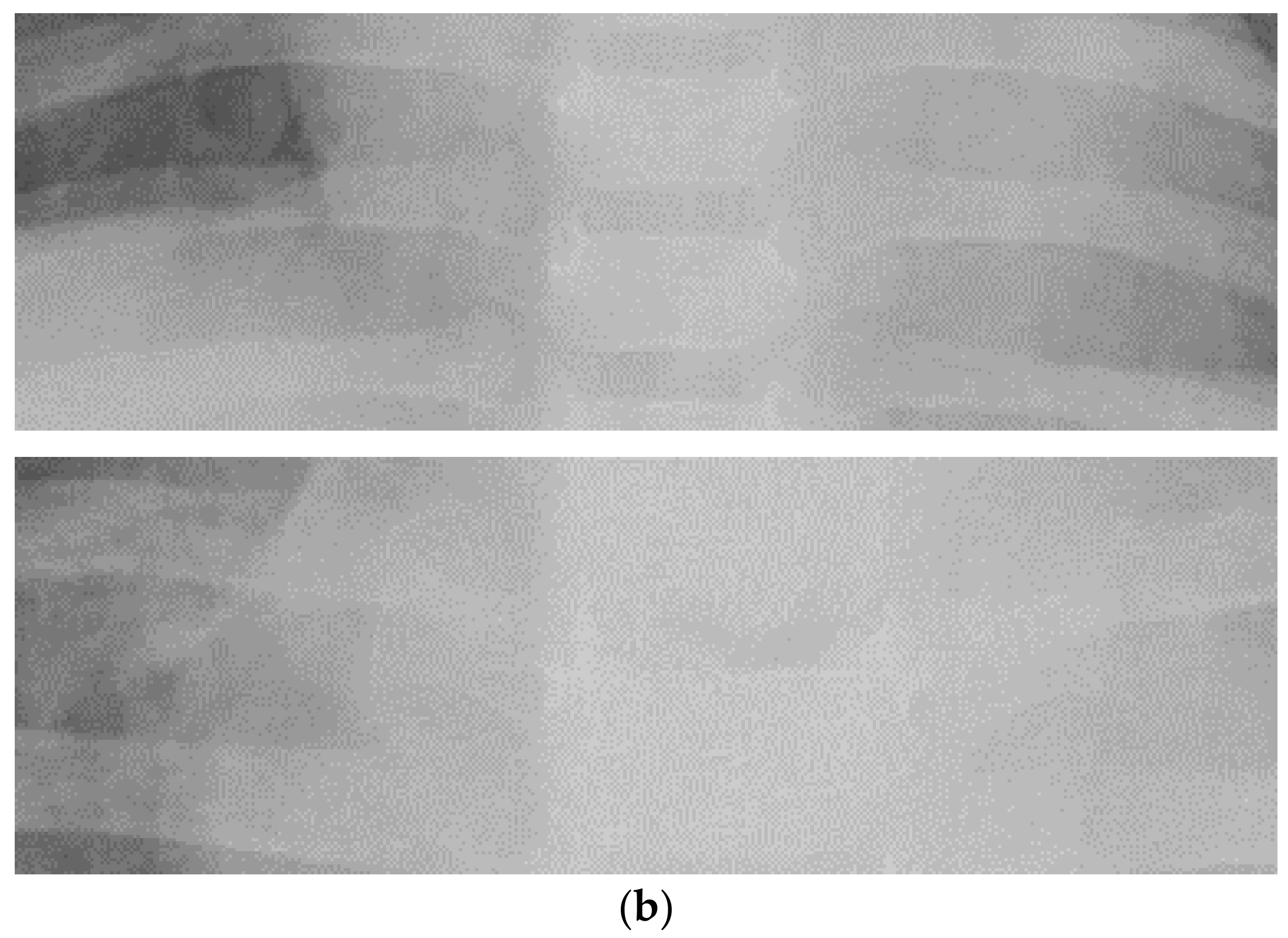
Figure 2 shows two FBIs of H = 17/64 and H = 25/64 with size 128 × 128 × 1; 
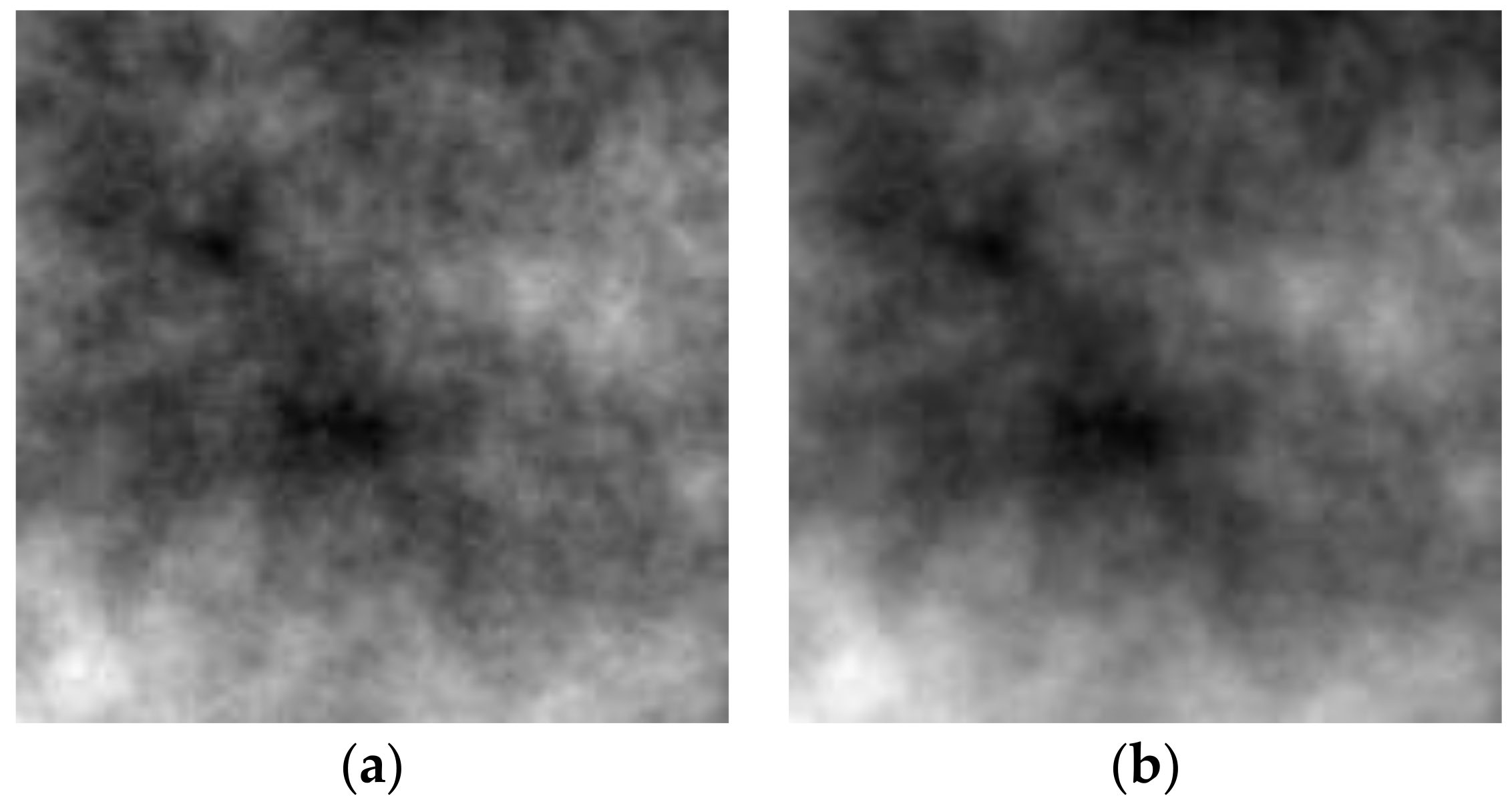
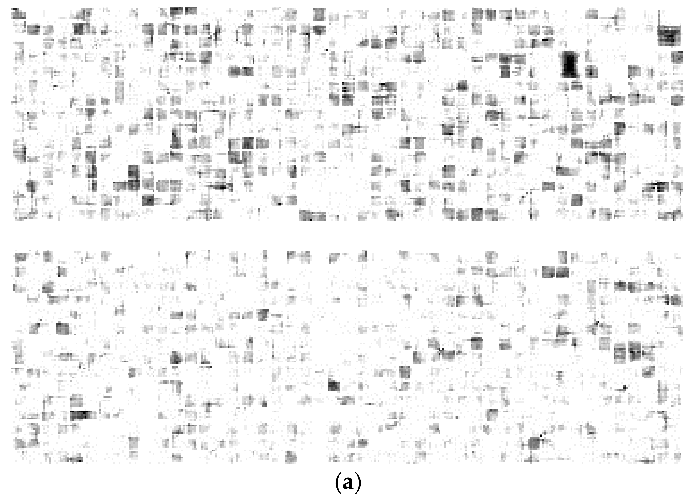
Figure 3 shows two FBIs of H = 33/64 and H = 41/64 with size 128 × 128 × 1; 
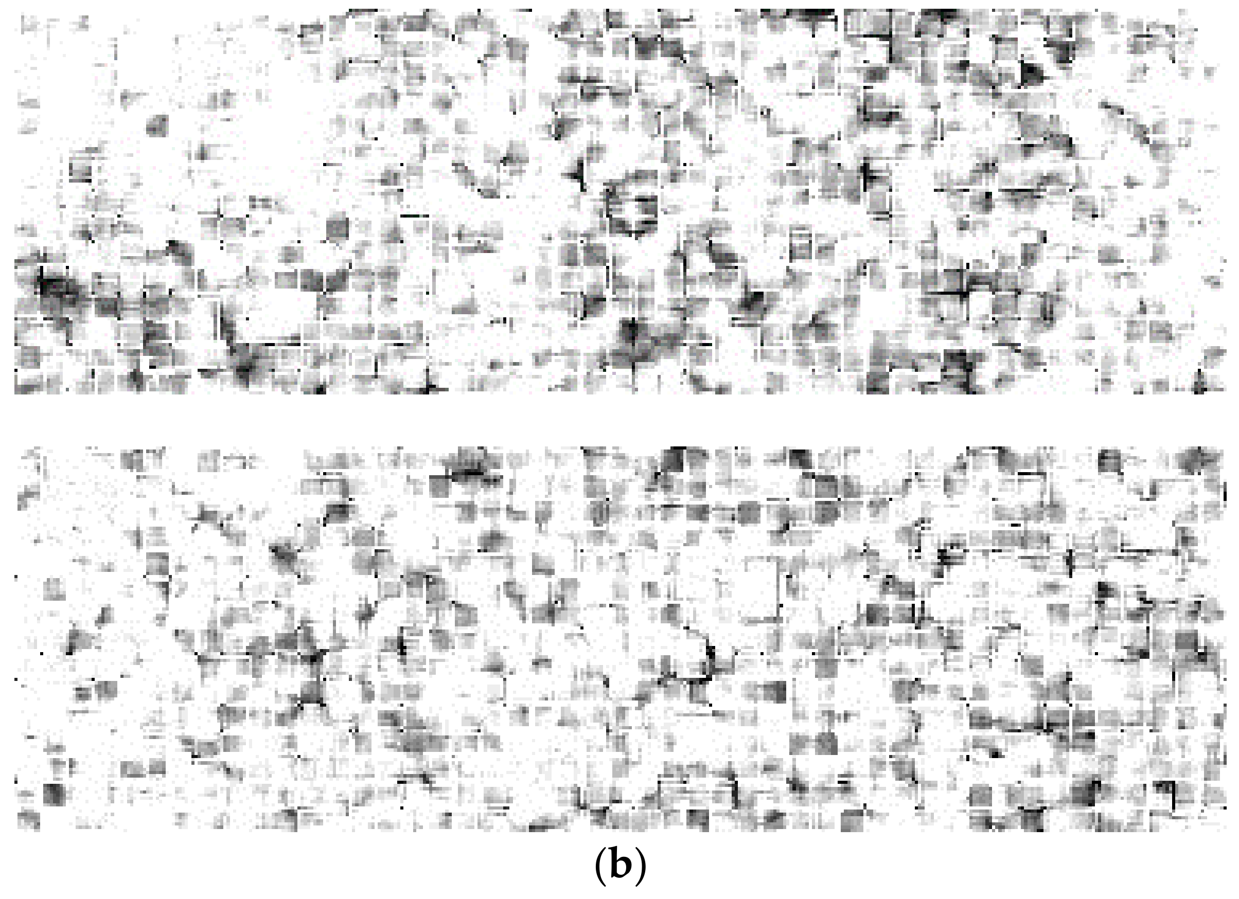
Figure 4 shows two FBIs of H = 49/64 and H = 57/64 with size 128 × 128 × 1. All eight FBIs were generated from the same realization or seed.
In Figure 1, Figure 2, Figure 3 and Figure 4, it is obvious that we cannot easily discriminate the images of two neighboring Hurst exponents with the naked eye, especially for higher Hurst exponents.
For a fair comparison, six deep-learning models were performed in the following operating environment: (1) a computer (Intel® Xeon(R) W-2235 CPU) with a GPU processor (NVIDIA RTX A4000) for running the models; (2) MATLAB R2022a for programming the models; (3) three solvers or optimizers [35,41] for training the models: sgdm, adaptive moment estimation (adam), and root mean square propagation (rmsprop); an initial learning rate of 0.001; a mini-batch size of 128; a piecewise learning rate schedule; a learning rate drop period of 20; a learning rate drop factor of 0.1; a shuffle for every epoch; number of epochs at 30; and a validation frequency of 30. For the efficient MLE, the comparison was performed in the same computing environment as outlined in points (1)–(3).

3.2. Results of the Maximum Likelihood Estimator

For comparison, two types of data were considered for the Hurst exponents: fractional Brownian surfaces (FBSs) and fractional Brownian images (FBIs), which are obtained from FBSs saved as gray-level images, thereby losing some finer details. Then, the efficient MLE for FBSs and FBIs was run under 11 Hurst exponents over five image sizes and 1000 observations. Since the efficient MLE will find out the optimal Hurst exponent between 0 and 1 through the golden section search, its computational time is terribly high for size 128 × 128 × 1, and hence, only the first 10 out of 1000 observations were estimated, not the complete 1000 observations.
Table 1 shows the MSEs for Set 1 and Set 2 over four image sizes (8 × 8, 16 × 16, 32 × 32, 64 × 64) under 1000 observations and over image size 128 × 128 × 1 under the first 10 out of 1000 observations. For example, under the same computing environment, our current computer will take about 646 s for the estimation of each observation, and hence, it will take at least 82 days to complete all 11000 estimations (11000 observations in total, 11 classes with 1000 observations each). This is another reason why we need the help of deep-learning models.
On the whole, the MSEs in Set 1 are similar to those in Set 2 for FBSs (true image data). As expected, the MSE decreases as the image size increases. However, this is not the case for FBIs because the higher Hurst exponents will lose many finer details with image size 64 × 64, leading to worse estimates from the efficient MLE. Obviously, the larger the size, the higher the loss.
It can be expected that the MSEs of FBSs will be smaller than those of FBIs because FBIs will lose some finer details, which are important for estimation by the efficient MLE. Moreover, the gaps between the MSEs of FBSs and FBIs will become larger as the image size increases, especially at 128 × 128. This is because more details are lost as the image size increases; our adopted estimator—the efficient MLE—cannot capture the finer structures of FBM. Although the performance with FBSs is far superior to that with FBIs, the data in the real world are mostly image data, not two-dimensional numerical data.

3.3. Results of Deep-Learning Models

The MLE is the best estimator for 2D FBM; it has the lowest MSE and is an unbiased estimator. The efficient MLE for 2D FBM is the fastest among the MLEs. Nevertheless, the computational costs are still extremely high, especially for larger image sizes. As the hardware for deep-learning models becomes quicker, and as deep-learning models become advanced and reliable, we will naturally pay more attention to this field and think of the ways in which the models can help us reduce the problem of computational costs.
In a previous pilot study [26] with only size 32 × 32 × 1 and three deep-learning models (one simple 29-layer model and two pre-trained models: AlexNet and GoogleNet) with solver or optimizer sgdm, we experimentally showed that deep-learning models are indeed feasible.
In the paper, we will try to design one 25-layer deep-learning model—which is simpler than previously designed models—and we will choose five pre-trained deep-learning models for a more comprehensive MSE comparison between the efficient MLE and deep-learning models, including five image sizes and three solvers (sgdm, adam, and rmsprop). In addition, we also want to know whether deep-learning models can learn the hidden realizations, i.e., whether deep-learning models do not see the validated data or observations (from different Hurst exponents) under five-fold cross-validation but possibly see partial realizations (i.e., partial white noise with the same seed was seen during training).
First, we develop a simple network mode—only 25 layers—consisting of four groups. The first group has one input layer; the second group is composed of four layers (a convolutional layer, a batch normalization layer, a ReLU layer, and a maximum pooling layer); the third group is composed of four layers (same as the second group without a maximum pooling layer); and finally, the fourth group is composed of three layers (a fully connected layer, a softmax layer, and a classification layer).
Based on the special structures of FBIs, we designed a simple model, consisting of regularly configured filters and increased sizes. Therefore, the input sizes of our proposed model include five image sizes (8 × 8 × 1, 16 × 16 × 1, 32 × 32 × 1, 64 × 64 × 1, and 128 × 128 × 1). From the first to the sixth convolutional layer, the filter numbers are all 128, with sizes from 3 × 3, 5 × 5, 7 × 7, 9 × 9, 11 × 11, to 13 × 13, respectively. In the future, we will try other combinations of filters and sizes, add other layers—such as dropout layers—and fine-tune their hyperparameters.
The size and stride of all maximum pooling layers are 2 × 2 and 2. According to the number of classes, the output size is 11 or 21. For more clarity, Table 2 shows the detailed architecture of our proposed model.
Based on our proposed 25-layer model, we run five-fold cross-validation on FBIs for five types of image sizes, each Hurst exponent with 1000 realizations from seed 1 to 1000 (Set 1). Under five-fold cross-validation, Table 3 and Table 4 show the classification rates of five folds and their mean and standard deviation for 11 classes and 21 classes, and Table 5 and Table 6 provide their corresponding MSEs of five folds and their mean and standard deviation for 11 classes and 21 classes. For MSEs, we first convert the classified classes to their corresponding Hurst exponents and then calculate the MSEs between the estimated Hurst exponents and the true Hurst exponents.
It is clear in Table 3 and Table 4 that the best accuracies of each solver all occur with size 16 × 16 × 1; that is, the proposed model is more suitable for size 16 × 16 × 1. Obviously, the simple design is not well suited for larger image sizes, such as 64 × 64 × 1 and 128 × 128 × 1, especially when the resolution is finer (21 Hurst exponents). Like all pre-trained models, no model can fit in all databases. Therefore, we can design different architectures of layers for other image sizes in terms of accuracies, MSEs, or other metrics.
Since the values of the Hurst exponent are continuous from 0 to 1, the classes are ordinal, not cardinal; the neighboring classes of the Hurst exponent are closer to each other than distant classes. Under ordinal classes, the misclassified classes of a good model should be closer to or neighboring the correct class. For ordinal classes, the classification rates are only one important indicator of reference, but the most practical metrics should be MSEs. Therefore, the corresponding MSEs for 11 classes and 21 classes—via the formula of MSEs versus classes—are listed for comparison in Table 5 and Table 6.
For a concise comparison, our proposed model was further summarized. Table 7 shows the summary of average accuracies for 11 and 21 classes over three solvers (sgdm, adam, and rmsprop), and Table 8 shows the summary of average MSEs (AMSEs, simply called MSEs) for 11 and 21 classes over three solvers (sgdm, adam, and rmsprop).
It is clear in Table 7 and Table 8 that the lowest MSE corresponds to the highest accuracy. For ordinal classes, the relationship between accuracies and MSEs is often used as an effective evaluation indicator for deep-learning models. The more consistent the relationship between accuracies and MSEs, the better designed the model is. Obviously, the proposed model is, on the whole, well designed and well performed.
On the other hand, the best MSEs occur at 16 × 16 × 1. This indicates that our proposed simple deep-learning model is more suited to smaller sizes. For other sizes, we need other more complex designs or the adoption of some ready-made or pre-trained models.
In addition, although the accuracies of 11 classes are all higher than those of 21 classes, the MSEs of 21 classes are all lower than those of 11 classes. For a well-designed model, this is very reasonable because the misclassified classes only occur at neighboring classes—not at remote classes. The spacing between two neighboring classes under 21 Hurst exponents is finer than that under 11 Hurst exponents. Accordingly, the MSEs will decrease. It can be reasonably expected that the MSEs for reliable deep-learning models will decrease as the resolution increases (or the spacing between two neighboring classes decreases), but for unqualified deep-learning models, the MSEs will possibly increase because these models prematurely converge or cannot converge during training. They will be implemented and discussed in future work.
Compared with MSEs of the MLE, our proposed simple 25-layer deep-learning model is much better than the MLE. This phenomenon may be due to two possibilities: one is that the correctly classified classes are zero errors; the other is that our proposed model can learn the hidden realizations because our model can see the partial realizations of seeds through five-fold cross-validation during training. Therefore, further evaluation is necessary for a fair comparison.
If the reason falls under the second possibility, it can be said experimentally that even a simple deep-learning model has the super power to learn the hidden realizations, not to mention the advanced pre-trained models.
After a simple deep-learning model was successfully proposed, we further experimented with three pre-trained models, which could be directly—without augmentation—run from size 8 × 8 × 1 to 128 × 128 × 1, and two pre-trained models, which could be directly run from size 32 × 32 × 1 to 128 × 128 × 1. The first group of pre-trained deep-learning models included Xception (71 layers deep, 170 layers in total), ResNet18 (18 layers deep, 71 layers in total), and MobileNetV2 (53 layers deep, 154 layers in total); the second group included GoogleNet (22 layers deep, 144 layers in total) and SqueezeNet (18 layers deep, 68 layers in total).
Since GoogleNet and SqueezeNet contain pooling layers—making the size smaller and smaller—GoogleNet and SqueezeNet are not suitable for sizes 8 × 8 × 1 and 16 × 16 × 1. Therefore, in the following four tables (Table 9, Table 10, Table 11 and Table 12), we use x to represent no experiment performed on the corresponding cell. In total, five pre-trained models were performed. All five pre-trained models were executed under five-fold cross-validation for the same FBIs. The sizes of our images for Xception, ResNet18, MobileNetV2 consisted of 8 × 8 × 1, 16 × 16 × 1, 32 × 32 × 1, 64 × 64 × 1, and 128 × 128 × 1. The sizes of our images for GoogleNet and SqueezeNet consisted of 32 × 32 × 1, 64 × 64 × 1, and 128 × 128 × 1. For a clear comparison, Table 9, Table 10, Table 11 and Table 12 contain six deep-learning models, including our proposed deep-learning model plus five pre-trained models.
All five pre-trained models were run under 11 classes and 21 classes. Their mean classification rates plus those of our proposed model are shown in Table 9 for 11 classes and in Table 10 for 21 classes. Their corresponding MSEs plus those of our proposed model are shown in Table 11 for 11 classes and in Table 12 for 21 classes. The corresponding detailed five-fold data of all five pre-trained models are arranged in Table A1, Table A2, Table A3, Table A4, Table A5, Table A6, Table A7, Table A8, Table A9, Table A10, Table A11, Table A12, Table A13, Table A14, Table A15, Table A16, Table A17, Table A18, Table A19 and Table A20 in Appendix A.
In the case of 11 classes, as mentioned previously, our proposed simple deep-learning model—only 25 layers—is more appropriate for smaller sizes, such as 8 × 8 × 1 and 16 × 16 × 1, as well as 32 × 32 × 1 only for the sgdm solver. MobileNetV2 (53 layers deep, 154 layers in total) exhibits an increasing classification rate as the size increases, and Xception (71 layers deep, 170 layers in total) exhibits a similar increasing trend, except with sizes 8 × 8 × 1 (9.10%) and 16 × 16 × 1 (9.09%) with the sgdm solver. This implies that models with deeper layers are beneficial for larger image sizes but detrimental for smaller image sizes. In particular, the sgdm solver is extremely unsuitable for Xception, as performed on our images.
ResNet18 (18 layers deep, 71 layers in total) also exhibits an increasing classification rate as the size increases when the solver is sgdm. When the solver adopted is adam, the best classification rate (99.01%) occurs at 64 × 64 × 1; when the solver adopted is rmsprop, the best classification rate (98.29%) actually occurs at 32 × 32 × 1.
GoogleNet (22 layers deep, 144 layers in total) and SqueezeNet (18 layers deep, 68 layers in total)—only run with data sizes 32 × 32 × 1, 64 × 64 × 1, and 128 × 128 × 1— also exhibit an increasing classification rate as the size increases. Their corresponding MSEs also reflect the trend. It is worth mentioning that an unstable result of mean 49.75% and standard deviation 20.50% occurs in SqueezeNet with the rmsprop solver at 32 × 32 × 1. Its five-fold classification rates are 18.09%, 77.50%, 55.50%, 60.95%, and 36.73% (see Table A5 in Appendix A).
In the case of 21 classes, their performance and trends are similar to those of 11 classes. ResNet18 also exhibits an increasing classification rate as the size increases when the solver is sgdm. When adam and rmsprop are chosen as solvers, their best classification rates of 96.87% and 96.29% both occur at 64 × 64 × 1.
GoogleNet exhibits an increasing classification rate as the size increases; the best classification rate is 95.67%. However, the best classification rate (97.28%) for the adam solver occurs at 64 × 64 × 1, while the best classification rate (91.90%) for the rmsprop solver occurs at 32 × 32 × 1.
In addition, an unstable result of mean 28.64% and standard deviation 23.20% occurs in SqueezeNet with the rmsprop solver at 32 × 32 × 1. Its five-fold classification rates are 4.76%, 57.14%, 4.76%, 21.64%, and 54.88% (see Table A10 in Appendix A).
Xception (71 layers deep, 170 layers in total) also exhibits an increasing trend as image sizes increase, except with sizes 8 × 8 × 1 (4.77%) and 16 × 16 × 1 (4.75%) with the sgdm solver. This also implies that models with deeper layers are beneficial for larger image sizes but detrimental for smaller image sizes. In particular, the sgdm solver is extremely unsuitable for Xception, as performed on our images. Relatively, the performance of MobileNetV2 (53 layers deep, 154 layers in total) steadily increases as the image size increases.
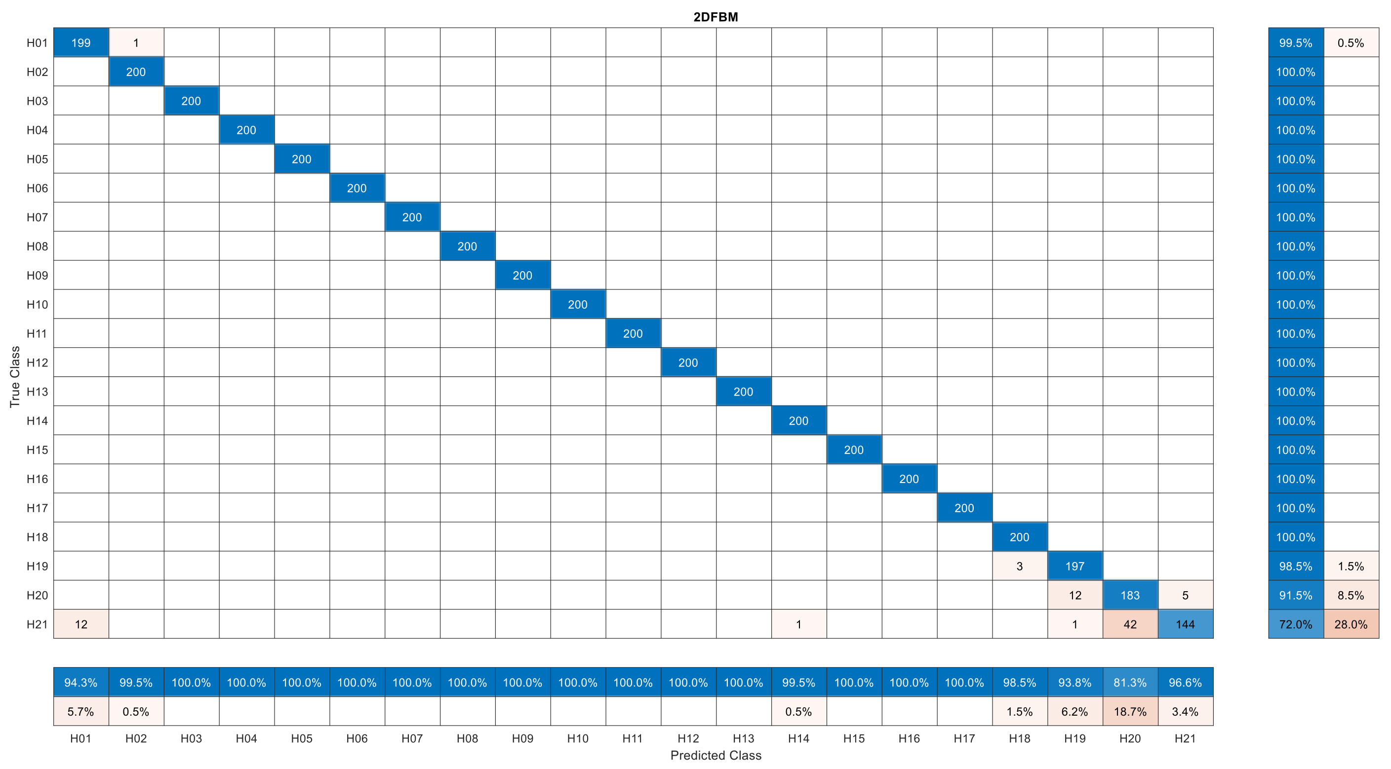
Upon careful observation of the case of Xception with the rmsprop solver with size 64 × 64 × 1 in Table 10 and Table 12, we find that it has the highest classification rate at 98.13%, but its corresponding MSE is 1.63 × 10−03—the largest among the six models and much higher than other models. This indicates that Xception with the rmsprop solver with size 64 × 64 × 1 is not reliable—even not qualified—for the ordinal classes in our image dataset. Figure 5 shows the confusion matrix in question from Fold 5. Blue cells stand for the numbers (diagonal) or percentages (vertical or horizontal) of correct classification and non-blue cells for the numbers or percentages of incorrect classification. The darker the color is, the higher the value. Obviously, the sharp increase mainly contributes to the reason for there being 12 class-21 images (H = 0.9762) classified as class 1 (H = 0.0238). This is a substantial mistake for our ordinal classes. It also indicates that a complex model under normal settings might not be suitable for our image dataset. For further applications, these kinds of complex models should be modified by fine-tuning their superparameters in order to achieve higher generalization ability.
As with Xception, some solvers are better, while some are worse. To avoid the potential problem of sensitivity or stability with solvers of deep-learning models, we consider the average accuracies and average MSEs (AMSEs, simply called MSEs) over three solvers (sgdm, adam, and rmsprop). Table 13 shows a summary of the six models for 11 classes, while Table 14 presents a summary of the six models for 21 classes. Table 15 shows a summary of the six models for 11 classes, while Table 16 presents a summary of the six models for 21 classes.
In Table 13 and Table 15, we find that each highest classification rate in Table 13 corresponds exactly to each smallest MSE in Table 15. Likewise, in Table 14 and Table 16, each highest classification rate in Table 14 corresponds almost exactly to each smallest MSE in Table 16, except for image size 32 × 32 × 1, where the highest classification rate is achieved in ResNet18, the second highest in GoogleNet, but the smallest MSE is achieved in GoogleNet, the second smallest in our proposed model, while ResNet18 only achieves the fifth smallest MSE.
If deep-learning models are stable for our image dataset, the MSEs of more classes (21 classes) should be smaller than those of fewer classes (11 classes). However, we find in Table 15 and Table 16 that there are five unstable cases: Xception at 64 × 64 × 1, ResNet18 at 32 × 32 × 1, and SqueezeNet at 32 × 32 × 1, 64 × 64 × 1, and 128 × 128 × 1. Stability is a very important indicator of which model we should adopt.
Compared to Table 1, except for some unstable cases—Xception at 8 × 8 × 1 and 16 × 16 × 1, as well as SqueezeNet at 32 × 32 × 1—our chosen five pre-trained models are almost superior to the true and best estimator (the MLE) in terms of MSEs. The results seem to be promising for the future. However, the calculation of MSEs via the formula of MSEs versus classes presents a potential unfair problem, in that the correctly classified classes in our situations are evaluated as zero errors, but those in real-world applications all contain certain errors. Accordingly, a further comparison is necessary.
In order to ascertain whether deep-learning models can learn the hidden realizations through different appearances or images (different Hurst exponents) with the same realizations, we evaluated the accuracies of Set 2 (seed 1001–2000) in models trained on Set 1 (seed 1–1000) with 11 classes. Table 17 shows the results, and Table 18 shows the corresponding differences between Table 17 (between-set evaluation) and Table 13 (within-set evaluation). For example, the first element of the first row in Table 17 and Table 13 is 37.83% and 92.70%, and hence, its difference is approximately −54.86%.
In Table 18, it is obvious that the accuracies of between-set evaluation are almost lower than those of within-set evaluation, except for our proposed model with size 128 × 128. Table 17 and Table 18 reveal to us that deep-learning models for smaller sizes can learn more hidden realizations from appearances or images, and hence, they can obtain higher accuracies even when they did not see the appearances in advance but did see some realizations through five-fold cross-validation during training. On the contrary, deep-learning models have a higher generalization ability for larger sizes because they can learn more detailed structures from their appearances, even when they did not see these realizations.
Now that deep-learning models have the ability to learn hidden realizations, for a fair and reasonable comparison, we additionally train three promising models (our proposed model, ResNet18, and MobileNetV2), each with five folds, on Set 1 (seed 1–1000) with 32 classes—hence five trained models for each deep-learning model—and then use Set 2 (seed 1001–2000) as our test set; that is, the trained models definitely did not see the appearances and their corresponding hidden realizations of the test or validation set (Set 2).
As mentioned before, the more classes of a qualified model there are, the lower its MSEs. Table 19 lists the average MSEs of the efficient MLE over 11,000 observations (except for size 128 × 128) and three deep-learning models over 165,000 (3 × 5 × 11,000) observations (three solvers and 11,000 observations per trained model from each fold); Table 20 lists the average computational times per observation of the efficient MLE and three deep-learning models. Since the efficient MLE for size 128 × 128 takes much longer (6.47 × 10+02 s per observation; at least 82 days for all 11,000 observations) to estimate, only the first 10 observations of each class were estimated for comparison.
In Table 19, we can observe that the MSEs of deep-learning models are almost lower than those of the efficient MLE for FBIs, except for size 32 × 32. In Table 1, we also find that the MSEs of these three deep-learning models for size 8 × 8 are also lower than those of the efficient MLE for FBSs (true image data). For size 16 × 16, our proposed model also results in lower MSE than the efficient MLE for FBSs, with MobileNetV2 presenting a slightly lower value.
In addition, the MSE of the MLE for FBIs increases as the size increases beyond 32 × 32 because FBIs lose the finer details when FBSs are stored as FBIs. Although deep-learning models cannot outperform the MLE for FBSs of larger sizes, the real-world data are generally images, not two-dimensional numerical data. The MSE of our proposed simple model almost decreases as the size increases, except for size 128 × 128, because our model is relatively simple (this may be overcome in the future by modifying the simple model structure). Nevertheless, it is still much better than the MLE for FBIs. For size 128 × 128, MobileNetV2 is the best choice in terms of MSE.
As mentioned before, our main purpose is to find an alternative to the estimated Hurst exponent from the efficient MLE because it will take a lot of time to estimate for larger sizes. Accordingly, time performance will play a very important indicator role in our study. It is obvious in Table 20 that the computational time of the efficient MLE increases as the size increases and that of the three models is approximately the same for all sizes. Therefore, the computational times of models are almost less than those of the efficient MLE, except for sizes smaller than 8 × 8 and 16 × 16. Our proposed model takes the least time among the three models.
In particular, the average computational time of each observation for size 128 × 128 takes 6.46 × 10+02 s, but that of our proposed model only takes 4.14 × 10−03 s. The time ratio of the efficient MLE to our proposed model is approximately 156,248—terribly high. Even for size 64 × 64, the time ratio of the efficient MLE to our proposed model is approximately 3090—still very high.
In terms of the computational time and MSE, our proposed simple deep-learning model should be recommended for indirectly estimating the Hurst exponent. In future, we may design some slightly complex models for sizes larger than 64 × 64 or choose some pre-trained models in order to achieve better MSEs within an acceptable time frame.

4. Discussion

The experimental results from Section 3 present us with an interesting phenomenon, namely that our proposed model can outperform the MLE even in FBSs with smaller sizes: 8 × 8 and 16 × 16. Therefore, in future, we would also like to know whether we can use the original data (FBSs) to train some deep-learning models to obtain fewer MSEs than the MLE.
When necessary, we typically use traditional estimators (also called direct estimators) to compute the fractal dimensions of images. For further classification, we use these estimates to classify their classes or types, such as benign and malignant. In the past, we often adopted the box-counting method for estimations because it is simple and efficient; however, it has considerably low accuracy, and therefore, it can only be applied in a domain with significant differences of fractal dimension. When applied to small differences, the box-counting method is often unreliable because of its considerably low accuracy, leading to a low recognition effect.
Lately, an efficient MLE for the Hurst exponent of 2D FBM was produced by Chang [24]. In theory, it is the optimal estimator, and to date, the fastest among the MLEs. However, its computational costs are still prohibitive, especially for larger image sizes, and hence, it is not applicable to fast analysis and evaluation. For example, in the current computing environment, it takes about 13.3 s for an image with size 64 × 64 and 646 s for an image with size 128 × 128. If the number of images needed to be estimated is not high, one can perhaps wait; however, the number is generally considerably high in real-world applications.
Sometimes, we would like to add an extra feature as our second input source in order to adopt two-stream models to enhance the classification effects. The extra feature may come from a fractal-dimension characteristic map of an original image. Therefore, it is extremely necessary to replace the traditional estimators with an effective and efficient approach, especially for larger images.
In the paper, we proposed one simple deep-learning model—only 25 layers—and selected five pre-trained models for comparison as well as a double check as to whether deep-learning models are appropriate as indirect estimators, including GoogleNet, Xception, MobileNetV2, ResNet18, and SqueezeNet.
In general, it is sufficient for fewer classes to analyze the differences between images by directly calculating the estimates through traditional well-performed estimators and then calculating their means and standard deviations. In this simple case, the step of classification through machine learning can be omitted. However, for many classes, it is better to classify these estimates using machine learning.
Machine-learning models depend on our manually chosen and extracted features—for example, the fractal dimension—but deep-learning models have the power to automatically capture as many features as possible. Therefore, if we find that deep-learning models perform well, we can use well-trained models to replace the role of the efficient MLE as an effective and efficient estimator in an indirect way, and further, as a characteristic transformer.
Recently, Chang and Jeng [26] designed a 29-layer sequential deep-learning model and selected three pre-trained networks—AlexNet, GoogleNet, and Xception—in order to prove experimentally that deep-learning models with the sgdm solver can work well for FBIs with size 32 × 32 × 1; additionally, the augmented GoogleNet was superior to the adjusted AlexNet and the augmented Xception in terms of the classification rate and computational cost. In their experiment, Chang and Jeng only used five-fold cross-validation within the same set to compare the performance between the efficient MLE and three models.
In the paper, we further designed a shallower model (25 layers as opposed to 29 implemented previously) and additionally selected three pre-trained models—ResNet18, MobileNetV2, and SqueezeNet—for comparison. In addition, the sizes of FBIs were expanded, including 8 × 8 × 1, 16 × 16 × 1, 32 × 32 × 1, 64 × 64 × 1, and 128 × 128 × 1 (five sizes in total). In addition, three widely used solvers—sgdm, adam, and rmsprop—were considered. Since AlexNet without augmentation cannot be run directly under these five original sizes, its comparison was excluded.
As we all know, these pre-trained models were trained under 1000 common object categories. They never saw the hidden structures of FBIs before, and hence, superficially, these models may work badly. Interestingly, they not only perform better than the efficient MLE for FBIs in terms of computational efficiency—except for smaller sizes on pre-trained models—but they also outperform the MLE in terms of effectiveness (based on MSEs), except for size 32 × 32, especially for larger sizes.
In the experiment conducted in the paper, we used two types of 11 and 21 Hurst exponents, each consisting of 1000 realizations with seed 1–1000 (Set 1), and we evaluated the models through five-fold cross-validation. For distinction, the evaluation method is called within-set evaluation; that is, a partial set (validation set) of Set 1 is evaluated on the other set (training set) of Set 1. Within-set evaluation shows that the best classification rates of the six deep-learning models with three solvers under 11 classes are 93.82% for 8 × 8 × 1, 97.35% for 16 × 16 × 1, 98.40% for 32 × 32 × 1, 99.41% for 64 × 64 × 1, and 99.88% for 128 × 128 × 1. Those under 21 classes are 91.75%, 95.30%, 97.59%, 98.28%, and 99.03%, respectively. For a fair comparison, for ordinal classes or continuous values, the mean-squared error (MSE) was also chosen as a metric. The MSEs of deep-learning models almost reflect their corresponding classification rates, except for Xception with the rmsprop solver. Their MSEs are all much better than those of the MLE.
When converting classes to MSEs for comparison with the MLE, there is some unfairness. For example, the correct classes are considered to be zero errors, but in practice, the estimations must contain certain errors. In addition, the realizations of every class come from the same seeds. We do not know whether deep-learning models have the power to learn the hidden realizations from different appearances (different Hurst exponents) with the same realizations.
To establish whether deep-learning models will learn the structure of realizations, the second set of realizations with seed 1001–2000 (Set 2) was used to generate another 11 classes of the Hurst exponent. The evaluation method is called between-set evaluation, in that the realizations from Set 2 were evaluated on deep-learning models trained on the realizations from Set 1. That is, one set (Set 2) is evaluated on another set (Set 1). The experimental results show that the average accuracies over three solvers under between-set evaluation are much lower than those under within-set evaluation, especially for smaller image sizes. The gaps between within-set and between-set evaluation confirm that deep-learning models will learn the structure of realizations even when they only indirectly saw them through the images of 2D FBM as opposed to seeing these realizations directly on their own.
The images of 2D FBM, unlike other data, are generated from white Gaussian noise through pseudo-random generators. Therefore, the same seed generates the same realization. During training, randomly grouping the images for five-fold cross-validation will lead to some realizations from the training set lying in the validation set in a direct way. Therefore, on the surface, deep-learning models with cross-validation did not see their validation data. In fact, they saw partial hidden realizations during training in an indirect way.
For a fair comparison, we further evaluated the realizations from Set 2 on deep-learning models trained on realizations from Set 1 with 32 classes; under 32 classes, it is impossible for data of 11 classes to be classified in the exact or correct class, and hence, no zero error occurs. The experimental results show that the MSEs of deep-learning models are almost lower than those of the MLE, except for images with size 32 × 32 × 1. Moreover, as the image size increases to more than 32 × 32 × 1, its MSE will increase, not decrease, because FBIs lose the finer details when they are stored from FBSs as FBIs.
In terms of computational costs, deep-learning models incur much lower costs than the efficient MLE, except for smaller image sizes on some pre-trained models, but our proposed model is always superior in efficiency to the efficient MLE, not to mention the MLE. The computational time of the deep-learning model is almost fixed for any image size, whereas that of the efficient MLE will increase as the image size increases; accordingly, the computational time of our proposed simple model is overwhelmingly lower than that of the efficient MLE—up to 156248 times with size 128 × 128 × 1. This is extremely high and cannot be ignored.
As we learned, when deep-learning models were run under the same realizations (within-set evaluation), they could obtain much higher classification rates and much lower MSEs, even though they had different appearances, but when they were run under different realizations (between-set evaluation), their classification rates and MSEs were considerably reduced. The results show that deep-learning models can learn the hidden realizations in an indirect way. For estimation, this is indeed a disadvantage, whereas it is an advantage for data hiding. In the applications of data hiding, we will indirectly hide some information in the classes of the Hurst exponent. When receiving the image of a certain class, a receiver can identify the class and then translate the class to the hidden information. The higher the classification rate, the more correct the interpreted information is. Therefore, when an attacker intercepts the image data, he/she cannot know what realizations were trained before, and hence, his/her interpretation will easily be erroneous. Therefore, in future, how to design deep-learning models will be a dilemma. This gives rise to an enormous challenge, but it also offers a substantial opportunity.
With the good performance of the deep-learning models, we will establish more model streams for one input image size to combine their respective advantages in order to enhance the overall performance in the upcoming future. For example, our proposed model is more suitable for smaller image sizes, while pre-trained models are all appropriate for middle-to-large image sizes. When well integrated together, the multiple model streams can be expected to be better than a single model stream. Moreover, we will consider more input resources, such as two image sizes for one model stream or multiple model streams, in order to explore more potential features.
Based on low MSEs and low computational costs, our well-designed simple deep-learning model and well-selected pre-trained deep-learning models can be widely applied in indirect estimations of the Hurst exponent. Different from traditional estimators, such as the MLE, our approach to estimating the Hurst exponent can therefore be viewed as simply a deep-learning estimator, or precisely, as an indirect deep-learning estimator from classes to Hurst exponents. Furthermore, as we know, different models will learn their own features according to their respective logic; hence, when indirectly estimating the Hurst exponents of practical images—often modeled as 2D FBM but seldom the exact model—they will look for diverse characteristic maps to help us explain more hidden details.
More importantly, the concept of deep-learning models as transformers—transforming the original images to the corresponding characteristic maps of the Hurst exponent—can be heavily promoted for other characteristic maps, such as the spectrum. Finally, through multiple input resources, the overall recognition rate of the original images combined with the corresponding characteristic maps will be highly increased for recognition of medical images. The idea will be explored in the upcoming future.
In general, our proposed simple deep-learning model is more suitable for smaller image sizes for classification and MSEs. This is reasonable because our proposed model only contains 25 layers, and no extra improvements or fine-tuning are imposed on the model. It can be expected that our proposed model can be improved further through other operations, such as adding dropout layers and modifying the related superparameters.
The excellent performance of the deep-learning models informs us that FBIs can still be learned from the curves and/or lines to capture hidden and subtle patterns from low to high layers. In terms of deep-learning models, it is unbelievable to learn the structure of these random processes, but it is a real fact.
Although we proposed a simple deep-learning model and selected five pre-trained models for classification, the corresponding MSEs also prove that our proposed model and selected pre-trained models are better than the MLE, except for size 32 × 32 × 1. At the moment, classification models—not regression models—are chosen because, on the one hand, most deep-learning models are well trained and designed for common object classification. Pre-trained models for classification can be directly adopted without any modification. From an intuitive viewpoint, using classification models followed by conversion of the classes into corresponding MSEs will give us smaller MSEs than using regression models. On the other hand, classifying the Hurst exponent provides potential applications for data hiding, and the higher the number of classes, the higher the amount of data hiding. Furthermore, this kind of data hiding is more difficult to break by the attackers.
In future, on the one hand, we will modify these pre-trained models for classification to those for regression in order to determine whether regression models are better than classification models. After all, our data type is ordinal—not cardinal. On the other hand, for data-hiding use, we will further study how to raise the classification rate of classes while increasing the number of classes for the Hurst exponent.

5. Potential Applications

As we know, some fractal characteristics often exist in the disease area of medical images, especially tumor development. They typically grow from small volumes into large volumes, and hence, we must detect them early and then treat them. If we want to discover the tiny changes, we need to differentiate the small differences between tissues. In the past, we could use traditional or direct estimators—such as the MLE or the box-counting method—to obtain fractal dimensions and then determine them via the distribution of these estimates, such as their means and standard deviations.
Since the MLE is the best estimator, and the efficient MLE is the most efficient among the MLEs, in the past, we would choose the efficient MLE for accuracy in order to estimate the Hurst exponent. However, its computation time often hinders its wide use, even standing still.
As the deep-learning models are becoming more and more advanced and mature, we experimentally proved that they could outperform the MLE for FBIs in the MSE, except for size 32 × 32 × 1. In addition, the computational cost of deep-learning models is kept almost constant as the image sizes increase, but the efficient MLE will increase these costs. When the size is 128 × 128 × 1, the computational time of the efficient MLE is about 156248 times that of our proposed model. For that reason, in future, we will replace the efficient MLE for FBIs with deep-learning models, especially our proposed simple model.
When medical images are modeled as FBIs, we can indirectly estimate the Hurst exponent by suitably selecting deep-learning models in an effective and efficient way. Although the fractal dimension (its value lies between 2 and 3) is more meaningful than its corresponding Hurst exponent (its value lies between 0 and 1) in terms of FBIs, the Hurst exponent is more suitable for elements of a feature map. For example, we selected from Kaggle [42] a database of chest X-rays as potential subjects. In order to exclude unimportant content from all images, we first established the smallest size—127 × 384—as our input size. Then, we clipped the central part of other images according to size. For illustration, we selected four clipped images as our subjects for transforming the original image to a feature map; Figure 6a presents two images from the normal group, and Figure 6b also presents two images from the pneumonia group.
In addition to the efficient MLE, we also selected three deep-learning models—our proposed model (25 layers), ResNet18, and MobileNetV2—run on 32 classes as our transformers, which converted the original images into their characteristic maps of the Hurst exponent. For transformation, we first chose 8 × 8 × 1 as the size of each sub-image for estimating the Hurst exponent. Second, we chose 1 × 1 as the stride or shift in the horizontal and vertical directions. From the top-left corner of the original image to the bottom-right corner, we estimated all the sub-images and saved these estimates as elements of the characteristic map.
In the first step, we directly estimated the Hurst exponents of all sub-images using the efficient MLE. In the second step, we indirectly estimated the Hurst exponents of all sub-images using the three deep-learning models mentioned above and then converted their classes to the corresponding Hurst exponents.
Figure 7, Figure 8, Figure 9 and Figure 10 show the feature/characteristic images or maps (120 × 377) generated using the efficient MLE and the three models. The lighter points are equivalent to the larger Hurst exponents; the darker points represent the smaller Hurst exponents.
Figure 7, Figure 8, Figure 9 and Figure 10 clearly show that these four sets of characteristic maps are not similar to one another. This is reasonable because practical images are not generally the exact images from the structure of 2D FBM. Therefore, the estimated Hurst exponents of all sub-images are generally different from one another. As we know, various deep-learning models will learn and capture various features from their respective viewpoints. For images with the exact characteristics of 2D FBM, deep-learning models can finally merge all the learned parameters into the correct classes, as the tables show. Therefore, even different deep-learning models obtain the same classes or Hurst exponents. However, when the sub-images are not the same images as 2D FBM, the results are usually different to one another, except for the learning structures of various models, which are similar to one another.
On the surface, four approaches—one traditional estimator, our proposed simple deep-learning model, two pre-trained deep-learning models—seem to give different explanations of the same image, but they all obey their peculiar logic to classify, or indirectly estimate, the Hurst exponent. Therefore, their interpretations all play very meaningful and important roles.
Although practical images modeled as a certain model—such as 2D FBM—are typically not ideal for their claimed model, their different characteristic appearances obtained seem to be good phenomena. Based on these various perspectives, through different models, we can extract diverse hidden characteristics. When cleverly integrated together, these various characteristic maps will give us much wider and richer resources for better analysis.
It is clear in Figure 6, Figure 7, Figure 8, Figure 9 and Figure 10 that these characteristic maps estimated by the efficient MLE or captured from the different trained learning models are simpler in essence than their original images. This is the most important quality of feature engineering [43]: expressing a problem in an easier and simpler way of understanding. For effective applications, feature engineering requires deep grasp of the nature of the problem [43]. For most medical images or some natural scenes, the Hurst exponent of 2D FBM is a very appropriate indicator. Therefore, the trained deep-learning models are effective as a tool of feature engineering.
For applications, two factors are important: effectiveness and efficiency. Naturally, we would also like to know the efficiency of models for feature engineering. As shown in Table 20, our proposed 25-layer model is obviously the smallest among the four approaches. In the case of size 8 × 8 × 1, only the computational time of our proposed model is less than that of the efficient MLE, but for larger sizes, deep-learning models are almost more efficient than the efficient MLE, except for MobileNetV2 with size 16 × 16 × 1. For size 128 × 128 × 1, the efficient MLE needs 156248 times more time than our proposed model, 69,018 times more than ResNet18, and 19211 times more than MobileNetV2.
In future, we will work hard to look for other deep-learning models for classification as well as for regression, and then, we will use the promising models to capture various features. Based on the diverse sources of features, we can integrate them with the original images to establish some successful multiple-stream or -input deep-learning models to classify more complex images in order to reach higher performance than a single-input model.

6. Conclusions

An efficient MLE for 2D FBM was recently proposed for direct estimations of Hurst exponents in place of the traditional MLE for higher efficiency. The MLE for 2D FBM is the optimal estimator in terms of performance, but its computational costs are still very high—enough to hinder adoption by users. Therefore, the purpose of the paper was to explore whether deep-learning models have the chance to overcome the problem of high computing costs within an acceptable time frame and with satisfactory accuracy.
In the paper, we proposed deep-learning estimators for the Hurst exponent of 2D FBM. First, we generated data of 2D FBM, called fractional Brownian surfaces (FBSs), then stored FBSs as images, simply called fractional Brownian images (FBIs). Since most pre-trained models were trained for 1000 object categories, we used deep-learning models for classification—not regression—to indirectly estimate the Hurst exponent by converting the classified classes to their corresponding Hurst exponents. Accordingly, we segmented the Hurst exponent into two groups of classes—11 classes and 21 classes—each class with equal spacing. For a fair comparison with the efficient maximum likelihood estimator (MLE) in terms of mean-squared errors (MSEs) and computational time, we also used one group of 32 equally spaced classes.
In the experiment, we used two sets of images, each class with 1000 FBIs from 1000 realizations generated by a pseudo-random generator with seed 1–1000, called Set 1. For further analysis and a fair comparison, we also generated the second set generated from seed 1001–2000, called Set 2. There were five image sizes considered, including 8 × 8 × 1, 16 × 16 × 1, 32 × 32 × 1, 64 × 64 × 1, and 128 × 128 × 1. Afterward, we designed one simple 25-layer deep-learning model and selected five pre-trained models—including Xception, ResNet18, MobileNetV2, GoogleNet, and SqueezeNet—to train these images under three common solvers: sgdm, adam, and rmsprop.
In the first experiment, we used five-fold cross-validation to evaluate six models on Set 1; the approach is called within-set evaluation. The experimental results showed that deep-learning models had very high classification rates, and their corresponding MSEs were much lower than those of the efficient MLE. To ascertain whether deep-learning models will learn the hidden realizations, in the second experiment, we used FBIs from Set 2 with 11 classes to evaluate the six models trained on Set 1; the approach is called between-set evaluation. Each deep-learning model contained five trained models, each fold with one trained model. Compared to within-set evaluation from the first experiment, between-set evaluation showed that the classification rates of deep-learning models decreased too much, especially for smaller image sizes. The big gaps between within-set and between-set evaluation confirmed that deep-learning models can learn the hidden realizations from different appearances based on different Hurst exponents, especially for smaller image sizes. This explained that deep-learning models have the power to learn hard-to-detect features even from a small part of background realizations.
In the previous two experiments, the correctly classified classes were given zero errors; however, any estimator—even the MLE—contains estimation errors. To avoid an unfair comparison with the MLE, in the third experiment, we used images from Set 2 to evaluate three models among the six models trained on 32 classes. Accordingly, no so-called correct class would appear, and hence, our experiment would be absolutely fair. The experimental results showed that the MSEs of three models were almost lower than those of the MLE, except for size 32 × 32 × 1. In addition, the computational efficiency of the three models was almost higher than that of the efficient MLE, except for smaller image sizes on two pre-trained models. Our proposed simple model is quite suitable for our case study of FBIs. The computational time of the efficient MLE was 156248, 69018, and 19211 times higher than that of our proposed model, ResNet18, and MobileNetV2 for size 128 × 128 × 1. This was terribly high. Therefore, deep-learning models are very suitable for replacing the efficient MLE for FBIs. In terms of FBSs, the subject merits another case study.
In terms of computational efficiency and accuracy, deep-learning models are indeed a good choice for indirectly estimating the Hurst exponent. In particular, when applied to larger datasets for transformers to transform the original images to characteristic maps, deep-learning models have a practical value. Time is money. The experimental results showed that lightweight models are more suitable for smaller image sizes. For example, the middle-size Xception under the rmsprop solver has high classification rates, but its MSEs will be higher than other lightweight models. In future, we will continue to consider larger image sizes to explore whether they require large-size models.

Funding

This work was supported by the National Science and Technology Council, Taiwan, Republic of China, under Grant NSTC 112-2221-E-040-008.

Data Availability Statement

Data are contained within the article.

Conflicts of Interest

The author declares no conflicts of interest.

Appendix A

Table A1. The five-fold classification rates for five types of image sizes and three solvers under 11 Hurst exponents: Xception.
SolversSizesFold 1Fold 2Fold 3Fold 4Fold 5MeanStd.
sgdm8 × 8 × 19.05%9.14%9.14%9.09%9.09%9.10%0.03%
16 × 16 × 19.09%9.09%9.05%9.09%9.14%9.09%0.03%
32 × 32 × 177.91%80.09%82.32%79.27%80.27%79.97%1.44%
64 × 64 × 187.14%87.68%87.64%85.27%86.73%86.89%0.88%
128 × 128 × 195.82%95.05%96.41%94.95%95.68%95.58%0.54%
adam8 × 8 × 184.05%80.86%77.27%82.86%83.09%81.63%2.41%
16 × 16 × 195.32%96.73%95.55%96.45%96.59%96.13%0.58%
32 × 32 × 198.23%98.68%98.41%99.00%97.68%98.40%0.44%
64 × 64 × 199.09%99.32%99.73%99.14%99.77%99.41%0.29%
128 × 128 × 199.86%99.95%99.77%99.82%100.00%99.88%0.08%
rmsprop8 × 8 × 176.64%77.23%77.14%82.41%79.59%78.60%2.16%
16 × 16 × 194.18%95.68%95.32%95.00%96.23%95.28%0.68%
32 × 32 × 198.59%98.86%97.18%98.45%97.64%98.15%0.63%
64 × 64 × 199.36%99.36%99.41%99.27%99.41%99.36%0.05%
128 × 128 × 199.82%99.86%99.64%99.86%99.77%99.79%0.08%
Table A2. The five-fold classification rates for five types of image sizes and three solvers under 11 Hurst exponents: ResNet18.
SolversSizesFold 1Fold 2Fold 3Fold 4Fold 5MeanStd.
sgdm8 × 8 × 158.68%59.45%59.68%59.82%58.86%59.30%0.45%
16 × 16 × 181.27%82.36%82.27%83.73%82.41%82.41%0.78%
32 × 32 × 191.95%91.68%92.64%92.32%90.64%91.85%0.69%
64 × 64 × 195.14%94.14%95.32%95.27%94.18%94.81%0.53%
128 × 128 × 197.23%97.50%97.86%97.55%97.36%97.50%0.21%
adam8 × 8 × 173.91%80.27%77.23%50.77%73.05%71.05%10.46%
16 × 16 × 192.73%88.64%81.82%92.91%93.27%89.87%4.37%
32 × 32 × 198.09%97.68%97.91%98.09%98.64%98.08%0.32%
64 × 64 × 198.41%99.09%98.95%98.77%99.82%99.01%0.46%
128 × 128 × 198.05%99.27%98.14%97.95%98.27%98.34%0.48%
rmsprop8 × 8 × 165.77%63.32%56.09%47.09%61.86%58.83%6.68%
16 × 16 × 191.36%93.00%92.41%92.41%92.36%92.31%0.53%
32 × 32 × 199.00%98.05%97.86%98.27%98.27%98.29%0.39%
64 × 64 × 198.86%97.59%96.55%98.59%99.14%98.15%0.96%
128 × 128 × 197.18%97.82%97.59%99.18%96.91%97.74%0.79%
Table A3. The five-fold classification rates for five types of image sizes and three solvers under 11 Hurst exponents: MobileNetV2.
SolversSizesFold 1Fold 2Fold 3Fold 4Fold 5MeanStd.
sgdm8 × 8 × 135.68%36.95%35.23%33.18%35.45%35.30%1.22%
16 × 16 × 168.95%63.91%68.09%70.18%68.59%67.95%2.13%
32 × 32 × 188.91%87.73%89.68%85.64%88.00%87.99%1.36%
64 × 64 × 194.86%94.55%95.27%95.36%94.55%94.92%0.35%
128 × 128 × 199.05%98.45%98.59%98.64%98.55%98.65%0.20%
adam8 × 8 × 132.55%35.27%32.41%32.23%38.95%34.28%2.59%
16 × 16 × 165.73%78.50%64.73%54.32%52.77%63.21%9.28%
32 × 32 × 196.45%96.18%94.23%95.55%95.64%95.61%0.77%
64 × 64 × 198.73%98.64%99.14%96.73%99.23%98.49%0.91%
128 × 128 × 199.73%99.77%99.23%99.45%99.73%99.58%0.21%
rmsprop8 × 8 × 148.55%58.77%45.18%55.55%45.32%50.67%5.53%
16 × 16 × 189.36%88.64%84.18%90.09%91.64%88.78%2.51%
32 × 32 × 197.18%97.05%97.36%97.68%97.05%97.26%0.24%
64 × 64 × 198.50%99.55%98.50%98.36%98.77%98.74%0.43%
128 × 128 × 199.45%99.50%99.64%99.50%99.50%99.52%0.06%
Table A4. The five-fold classification rates for five types of image sizes and three solvers under 11 Hurst exponents: GoogleNet.
SolversSizesFold 1Fold 2Fold 3Fold 4Fold 5MeanStd.
sgdm32 × 32 × 192.41%92.68%92.95%91.50%93.45%92.60%0.65%
64 × 64 × 196.50%96.32%97.91%96.82%97.50%97.01%0.60%
128 × 128 × 199.09%98.73%99.00%98.64%98.82%98.85%0.17%
adam32 × 32 × 195.64%96.27%97.27%96.45%95.82%96.29%0.57%
64 × 64 × 198.09%98.18%98.59%97.82%99.09%98.35%0.44%
128 × 128 × 199.32%99.05%99.18%99.05%98.00%98.92%0.47%
rmsprop32 × 32 × 191.86%91.59%92.68%90.41%91.41%91.59%0.73%
64 × 64 × 194.91%94.41%95.05%92.59%97.05%94.80%1.42%
128 × 128 × 197.64%95.32%96.91%96.59%96.05%96.50%0.78%
Table A5. The five-fold classification rates for five types of image sizes and three solvers under 11 Hurst exponents: SqueezeNet.
SolversSizesFold 1Fold 2Fold 3Fold 4Fold 5MeanStd.
sgdm32 × 32 × 184.05%85.50%85.00%86.86%86.32%85.55%0.99%
64 × 64 × 197.23%96.45%97.64%96.73%97.82%97.17%0.52%
128 × 128 × 198.50%96.14%98.95%98.73%98.00%98.06%1.01%
adam32 × 32 × 194.23%94.95%87.95%93.59%94.05%92.95%2.54%
64 × 64 × 198.59%98.91%98.55%98.32%98.95%98.66%0.24%
128 × 128 × 199.05%99.27%99.64%99.41%99.36%99.35%0.19%
rmsprop32 × 32 × 118.09%77.50%55.50%60.95%36.73%49.75%20.50%
64 × 64 × 196.23%95.64%96.18%95.82%97.32%96.24%0.58%
128 × 128 × 198.32%97.86%99.14%97.77%98.32%98.28%0.48%
Table A6. The five-fold classification rates for five types of image sizes and three solvers under 21 Hurst exponents: Xception.
SolversSizesFold 1Fold 2Fold 3Fold 4Fold 5MeanStd.
sgdm8 × 8 × 14.79%4.79%4.76%4.76%4.76%4.77%0.01%
16 × 16 × 14.76%4.74%4.74%4.76%4.76%4.75%0.01%
32 × 32 × 182.60%81.64%81.33%83.81%82.36%82.35%0.86%
64 × 64 × 187.71%88.55%87.86%88.64%84.40%87.43%1.56%
128 × 128 × 193.98%94.17%94.24%94.36%93.98%94.14%0.15%
adam8 × 8 × 176.48%78.55%77.24%80.14%78.26%78.13%1.25%
16 × 16 × 195.26%94.62%93.76%94.43%95.71%94.76%0.68%
32 × 32 × 197.21%96.64%98.36%97.48%98.26%97.59%0.65%
64 × 64 × 198.88%98.21%97.33%98.38%98.60%98.28%0.52%
128 × 128 × 199.10%99.14%98.90%98.95%99.07%99.03%0.09%
rmsprop8 × 8 × 178.88%78.07%79.36%77.62%76.55%78.10%0.98%
16 × 16 × 195.24%93.81%95.05%93.36%95.57%94.60%0.86%
32 × 32 × 197.76%94.86%97.48%96.36%97.31%96.75%1.06%
64 × 64 × 198.50%98.02%97.81%97.29%99.05%98.13%0.60%
128 × 128 × 199.05%98.90%99.14%97.38%99.19%98.73%0.68%
Table A7. The five-fold classification rates for five types of image sizes and three solvers under 21 Hurst exponents: ResNet18.
SolversSizesFold 1Fold 2Fold 3Fold 4Fold 5MeanStd.
sgdm8 × 8 × 160.50%63.33%64.45%57.81%63.60%61.94%2.45%
16 × 16 × 182.31%83.88%84.21%82.86%81.31%82.91%1.06%
32 × 32 × 192.24%91.05%91.40%91.60%90.57%91.37%0.56%
64 × 64 × 195.00%94.62%94.90%94.36%93.62%94.50%0.49%
128 × 128 × 195.29%96.24%95.98%96.17%96.24%95.98%0.36%
adam8 × 8 × 160.62%79.48%74.81%71.86%64.12%70.18%6.91%
16 × 16 × 174.76%84.64%86.43%82.76%88.79%83.48%4.79%
32 × 32 × 196.93%97.38%96.67%95.00%95.57%96.31%0.89%
64 × 64 × 198.64%96.26%96.31%95.36%97.76%96.87%1.18%
128 × 128 × 195.83%94.64%96.64%91.29%94.48%94.58%1.83%
rmsprop8 × 8 × 170.43%72.64%71.17%78.05%75.33%73.52%2.82%
16 × 16 × 188.33%80.29%86.38%84.67%84.52%84.84%2.66%
32 × 32 × 197.55%93.31%96.07%95.33%95.19%95.49%1.37%
64 × 64 × 198.21%91.93%96.05%97.43%97.81%96.29%2.30%
128 × 128 × 195.83%95.57%90.12%96.10%90.00%93.52%2.83%
Table A8. The five-fold classification rates for five types of image sizes and three solvers under 21 Hurst exponents: MobileNetV2.
SolversSizesFold 1Fold 2Fold 3Fold 4Fold 5MeanStd.
sgdm8 × 8 × 131.14%32.29%34.02%34.29%32.40%32.83%1.17%
16 × 16 × 168.21%66.38%67.21%67.14%67.02%67.20%0.59%
32 × 32 × 186.60%82.79%88.26%86.88%87.95%86.50%1.96%
64 × 64 × 193.12%92.93%93.12%92.88%93.64%93.14%0.27%
128 × 128 × 195.48%95.07%96.17%96.21%95.48%95.68%0.44%
adam8 × 8 × 121.21%17.95%21.81%40.57%29.40%26.19%8.11%
16 × 16 × 147.45%57.74%64.38%74.02%52.95%59.31%9.23%
32 × 32 × 191.36%82.95%87.19%91.45%93.36%89.26%3.74%
64 × 64 × 195.43%95.88%97.60%97.24%97.24%96.68%0.86%
128 × 128 × 198.67%98.05%98.64%99.07%98.05%98.50%0.40%
rmsprop8 × 8 × 162.52%57.12%63.50%49.57%63.31%59.20%5.36%
16 × 16 × 183.05%79.29%87.14%84.93%86.43%84.17%2.82%
32 × 32 × 190.88%94.48%96.62%94.00%94.29%94.05%1.84%
64 × 64 × 195.57%96.71%97.64%96.05%96.62%96.52%0.70%
128 × 128 × 198.40%98.00%98.55%97.69%97.60%98.05%0.38%
Table A9. The five-fold classification rates for five types of image sizes and three solvers under 21 Hurst exponents: GoogleNet.
SolversSizesFold 1Fold 2Fold 3Fold 4Fold 5MeanStd.
sgdm32 × 32 × 192.60%91.40%93.24%92.76%92.17%92.43%0.62%
64 × 64 × 195.26%95.05%94.88%94.83%95.21%95.05%0.17%
128 × 128 × 195.98%95.60%95.48%95.36%95.93%95.67%0.25%
adam32 × 32 × 195.71%95.67%96.50%96.38%96.19%96.09%0.34%
64 × 64 × 197.40%97.17%97.05%97.21%97.57%97.28%0.19%
128 × 128 × 197.10%97.10%96.29%96.45%96.95%96.78%0.34%
rmsprop32 × 32 × 191.90%91.21%93.45%91.38%91.57%91.90%0.81%
64 × 64 × 189.43%87.14%87.93%89.10%89.90%88.70%1.02%
128 × 128 × 190.52%91.69%90.38%90.24%91.69%90.90%0.65%
Table A10. The five-fold classification rates for five types of image sizes and three solvers under 21 Hurst exponents: SqueezeNet.
SolversSizesFold 1Fold 2Fold 3Fold 4Fold 5MeanStd.
sgdm32 × 32 × 172.83%68.07%74.14%81.10%77.67%74.76%4.41%
64 × 64 × 188.76%89.29%88.50%88.69%86.69%88.39%0.89%
128 × 128 × 194.31%92.62%93.52%93.48%93.45%93.48%0.54%
adam32 × 32 × 184.10%74.05%64.74%74.21%85.36%76.49%7.56%
64 × 64 × 196.24%96.29%96.74%96.05%95.55%96.17%0.39%
128 × 128 × 197.60%96.24%97.29%97.52%97.43%97.21%0.50%
rmsprop32 × 32 × 14.76%57.14%4.76%21.64%54.88%28.64%23.20%
64 × 64 × 184.31%83.33%85.43%83.79%83.67%84.10%0.73%
128 × 128 × 191.17%91.69%92.10%92.67%92.90%92.10%0.63%
Table A11. The five-fold MSEs for five types of image sizes and three solvers under 11 Hurst exponents: Xception.
SolversSizesFold 1Fold 2Fold 3Fold 4Fold 5MeanStd.
sgdm8 × 8 × 11.57 × 10−012.89 × 10−012.15 × 10−019.10 × 10−028.28 × 10−021.67 × 10−017.76 × 10−02
16 × 16 × 11.57 × 10−012.89 × 10−012.15 × 10−019.17 × 10−028.27 × 10−021.67 × 10−017.76 × 10−02
32 × 32 × 12.52 × 10−032.07 × 10−031.75 × 10−032.13 × 10−032.02 × 10−032.10 × 10−032.50 × 10−04
64 × 64 × 11.07 × 10−031.04 × 10−031.03 × 10−031.25 × 10−031.11 × 10−031.10 × 10−037.94 × 10−05
128 × 128 × 13.46 × 10−044.09 × 10−042.97 × 10−044.17 × 10−043.57 × 10−043.65 × 10−044.42 × 10−05
adam8 × 8 × 11.65 × 10−032.07 × 10−032.46 × 10−032.62 × 10−032.03 × 10−032.17 × 10−033.40 × 10−04
16 × 16 × 14.09 × 10−042.70 × 10−043.68 × 10−043.27 × 10−043.16 × 10−043.38 × 10−044.73 × 10−05
32 × 32 × 11.47 × 10−041.09 × 10−041.31 × 10−048.26 × 10−051.92 × 10−041.32 × 10−043.67 × 10−05
64 × 64 × 17.51 × 10−055.63 × 10−052.25 × 10−057.14 × 10−051.88 × 10−054.88 × 10−052.39 × 10−05
128 × 128 × 11.13 × 10−053.76 × 10−061.88 × 10−051.50 × 10−050.00 × 10+009.77 × 10−066.97 × 10−06
rmsprop8 × 8 × 12.47 × 10−032.47 × 10−032.58 × 10−031.83 × 10−032.34 × 10−032.34 × 10−032.66 × 10−04
16 × 16 × 15.03 × 10−047.51 × 10−045.67 × 10−048.08 × 10−043.57 × 10−045.97 × 10−041.65 × 10−04
32 × 32 × 11.16 × 10−049.39 × 10−052.33 × 10−041.28 × 10−042.07 × 10−041.56 × 10−045.42 × 10−05
64 × 64 × 15.26 × 10−055.26 × 10−054.88 × 10−056.01 × 10−054.88 × 10−055.26 × 10−054.12 × 10−06
128 × 128 × 11.50 × 10−051.13 × 10−053.01 × 10−051.13 × 10−051.88 × 10−051.73 × 10−056.97 × 10−06
Table A12. The five-fold MSEs for five types of image sizes and three solvers under 11 Hurst exponents: ResNet18.
SolversSizesFold 1Fold 2Fold 3Fold 4Fold 5MeanStd.
sgdm8 × 8 × 15.66 × 10−035.52 × 10−035.62 × 10−035.54 × 10−035.60 × 10−035.59 × 10−035.06 × 10−05
16 × 16 × 11.98 × 10−031.68 × 10−031.59 × 10−031.54 × 10−031.75 × 10−031.71 × 10−031.56 × 10−04
32 × 32 × 16.65 × 10−047.33 × 10−046.54 × 10−046.46 × 10−047.96 × 10−046.99 × 10−045.77 × 10−05
64 × 64 × 14.13 × 10−044.85 × 10−043.87 × 10−043.91 × 10−044.81 × 10−044.31 × 10−044.30 × 10−05
128 × 128 × 12.29 × 10−042.07 × 10−041.77 × 10−042.03 × 10−042.18 × 10−042.07 × 10−041.76 × 10−05
adam8 × 8 × 12.76 × 10−032.09 × 10−032.73 × 10−037.01 × 10−033.02 × 10−033.52 × 10−031.77 × 10−03
16 × 16 × 16.80 × 10−049.84 × 10−041.54 × 10−036.20 × 10−046.35 × 10−048.91 × 10−043.49 × 10−04
32 × 32 × 11.58 × 10−041.92 × 10−041.84 × 10−041.58 × 10−041.13 × 10−041.61 × 10−042.76 × 10−05
64 × 64 × 11.31 × 10−047.51 × 10−058.64 × 10−051.01 × 10−041.50 × 10−058.19 × 10−053.84 × 10−05
128 × 128 × 11.62 × 10−046.01 × 10−051.54 × 10−041.69 × 10−041.43 × 10−041.37 × 10−043.97 × 10−05
rmsprop8 × 8 × 13.99 × 10−035.03 × 10−036.12 × 10−038.19 × 10−035.02 × 10−035.67 × 10−031.43 × 10−03
16 × 16 × 18.38 × 10−046.35 × 10−046.50 × 10−046.50 × 10−046.76 × 10−046.90 × 10−047.52 × 10−05
32 × 32 × 18.26 × 10−051.62 × 10−041.77 × 10−041.43 × 10−041.43 × 10−041.41 × 10−043.19 × 10−05
64 × 64 × 19.39 × 10−051.99 × 10−042.85 × 10−041.16 × 10−047.14 × 10−051.53 × 10−047.90 × 10−05
128 × 128 × 12.33 × 10−041.80 × 10−041.99 × 10−046.76 × 10−052.55 × 10−041.87 × 10−046.52 × 10−05
Table A13. The five-fold MSEs for five types of image sizes and three solvers under 11 Hurst exponents: MobileNetV2.
SolversSizesFold 1Fold 2Fold 3Fold 4Fold 5MeanStd.
sgdm8 × 8 × 11.24 × 10−021.08 × 10−021.23 × 10−021.43 × 10−021.23 × 10−021.24 × 10−021.11 × 10−03
16 × 16 × 12.93 × 10−033.50 × 10−033.11 × 10−032.86 × 10−033.04 × 10−033.09 × 10−032.23 × 10−04
32 × 32 × 19.50 × 10−041.01 × 10−038.53 × 10−041.19 × 10−039.92 × 10−049.99 × 10−041.09 × 10−04
64 × 64 × 14.24 × 10−044.51 × 10−043.91 × 10−043.83 × 10−044.51 × 10−044.20 × 10−042.87 × 10−05
128 × 128 × 17.89 × 10−051.28 × 10−041.16 × 10−041.13 × 10−041.20 × 10−041.11 × 10−041.69 × 10−05
adam8 × 8 × 11.76 × 10−021.60 × 10−021.90 × 10−022.04 × 10−021.25 × 10−021.71 × 10−022.74 × 10−03
16 × 16 × 13.43 × 10−031.98 × 10−033.66 × 10−035.23 × 10−035.50 × 10−033.96 × 10−031.29 × 10−03
32 × 32 × 13.04 × 10−043.27 × 10−044.88 × 10−043.68 × 10−043.61 × 10−043.70 × 10−046.37 × 10−05
64 × 64 × 11.05 × 10−041.13 × 10−047.14 × 10−052.70 × 10−046.39 × 10−051.25 × 10−047.53 × 10−05
128 × 128 × 12.25 × 10−051.88 × 10−056.39 × 10−054.51 × 10−052.25 × 10−053.46 × 10−051.74 × 10−05
rmsprop8 × 8 × 17.07 × 10−035.29 × 10−039.17 × 10−036.44 × 10−038.56 × 10−037.30 × 10−031.41 × 10−03
16 × 16 × 19.58 × 10−041.02 × 10−031.41 × 10−038.41 × 10−047.14 × 10−049.88 × 10−042.35 × 10−04
32 × 32 × 12.33 × 10−042.44 × 10−042.18 × 10−041.92 × 10−042.44 × 10−042.26 × 10−041.98 × 10−05
64 × 64 × 11.24 × 10−043.76 × 10−051.24 × 10−041.35 × 10−041.01 × 10−041.04 × 10−043.52 × 10−05
128 × 128 × 14.51 × 10−054.13 × 10−053.01 × 10−054.13 × 10−054.13 × 10−053.98 × 10−055.10 × 10−06
Table A14. The five-fold MSEs for five types of image sizes and three solvers under 11 Hurst exponents: GoogleNet.
SolversSizesFold 1Fold 2Fold 3Fold 4Fold 5MeanStd.
sgdm32 × 32 × 16.39 × 10−046.05 × 10−045.82 × 10−047.02 × 10−045.41 × 10−046.14 × 10−045.45 × 10−05
64 × 64 × 12.89 × 10−043.04 × 10−041.73 × 10−042.63 × 10−042.07 × 10−042.47 × 10−044.99 × 10−05
128 × 128 × 17.51 × 10−051.05 × 10−048.26 × 10−051.13 × 10−049.77 × 10−059.47 × 10−051.39 × 10−05
adam32 × 32 × 13.61 × 10−043.08 × 10−042.25 × 10−042.93 × 10−043.46 × 10−043.07 × 10−044.74 × 10−05
64 × 64 × 11.58 × 10−041.50 × 10−041.16 × 10−041.80 × 10−047.51 × 10−051.36 × 10−043.67 × 10−05
128 × 128 × 15.63 × 10−057.89 × 10−056.76 × 10−057.89 × 10−051.65 × 10−048.94 × 10−053.89 × 10−05
rmsprop32 × 32 × 16.84 × 10−047.29 × 10−046.16 × 10−048.04 × 10−047.21 × 10−047.11 × 10−046.13 × 10−05
64 × 64 × 14.21 × 10−044.62 × 10−044.09 × 10−046.12 × 10−042.44 × 10−044.30 × 10−041.18 × 10−04
128 × 128 × 11.95 × 10−043.87 × 10−042.55 × 10−042.82 × 10−043.27 × 10−042.89 × 10−046.48 × 10−05
Table A15. The five-fold MSEs for five types of image sizes and three solvers under 11 Hurst exponents: SqueezeNet.
SolversSizesFold 1Fold 2Fold 3Fold 4Fold 5MeanStd.
sgdm32 × 32 × 11.33 × 10−031.21 × 10−031.24 × 10−031.09 × 10−031.13 × 10−031.20 × 10−038.53 × 10−05
64 × 64 × 12.29 × 10−042.93 × 10−041.95 × 10−042.70 × 10−041.80 × 10−042.34 × 10−044.29 × 10−05
128 × 128 × 11.24 × 10−043.19 × 10−048.64 × 10−051.05 × 10−041.65 × 10−041.60 × 10−048.38 × 10−05
adam32 × 32 × 14.77 × 10−044.17 × 10−045.40 × 10−025.30 × 10−044.92 × 10−041.12 × 10−022.14 × 10−02
64 × 64 × 11.16 × 10−049.02 × 10−051.20 × 10−041.39 × 10−048.64 × 10−051.10 × 10−041.97 × 10−05
128 × 128 × 17.89 × 10−056.01 × 10−053.01 × 10−054.88 × 10−055.26 × 10−055.41 × 10−051.59 × 10−05
rmsprop32 × 32 × 11.31 × 10−012.24 × 10−028.96 × 10−025.54 × 10−026.56 × 10−027.28 × 10−023.62 × 10−02
64 × 64 × 13.12 × 10−043.61 × 10−043.16 × 10−043.46 × 10−042.22 × 10−043.11 × 10−044.83 × 10−05
128 × 128 × 11.39 × 10−041.77 × 10−047.14 × 10−051.84 × 10−041.39 × 10−041.42 × 10−043.99 × 10−05
Table A16. The five-fold MSEs for five types of image sizes and three solvers under 21 Hurst exponents: Xception.
SolversSizesFold 1Fold 2Fold 3Fold 4Fold 5MeanStd.
sgdm8 × 8 × 19.27 × 10−028.57 × 10−021.04 × 10−011.20 × 10−011.04 × 10−011.01 × 10−011.15 × 10−02
16 × 16 × 19.23 × 10−028.59 × 10−021.04 × 10−011.20 × 10−011.04 × 10−011.01 × 10−011.15 × 10−02
32 × 32 × 19.94 × 10−046.90 × 10−041.09 × 10−035.48 × 10−046.33 × 10−047.92 × 10−042.13 × 10−04
64 × 64 × 12.96 × 10−043.20 × 10−043.01 × 10−042.72 × 10−043.86 × 10−043.15 × 10−043.86 × 10−05
128 × 128 × 11.37 × 10−041.36 × 10−041.32 × 10−041.28 × 10−041.38 × 10−041.34 × 10−043.64 × 10−06
adam8 × 8 × 11.23 × 10−037.76 × 10−048.41 × 10−047.30 × 10−048.33 × 10−048.81 × 10−041.77 × 10−04
16 × 16 × 11.28 × 10−041.68 × 10−041.88 × 10−041.61 × 10−041.25 × 10−041.54 × 10−042.44 × 10−05
32 × 32 × 16.80 × 10−058.58 × 10−054.21 × 10−056.69 × 10−054.70 × 10−056.20 × 10−051.58 × 10−05
64 × 64 × 12.54 × 10−054.05 × 10−056.05 × 10−053.67 × 10−053.19 × 10−053.90 × 10−051.19 × 10−05
128 × 128 × 12.05 × 10−051.94 × 10−052.48 × 10−052.38 × 10−052.11 × 10−052.19 × 10−052.04 × 10−06
rmsprop8 × 8 × 17.60 × 10−048.29 × 10−049.17 × 10−041.49 × 10−038.71 × 10−049.73 × 10−042.63 × 10−04
16 × 16 × 11.24 × 10−041.39 × 10−031.46 × 10−043.03 × 10−031.49 × 10−049.70 × 10−041.14 × 10−03
32 × 32 × 15.56 × 10−053.47 × 10−046.05 × 10−059.34 × 10−057.02 × 10−051.25 × 10−041.11 × 10−04
64 × 64 × 13.40 × 10−054.81 × 10−055.19 × 10−032.86 × 10−032.16 × 10−051.63 × 10−032.09 × 10−03
128 × 128 × 12.16 × 10−052.48 × 10−051.94 × 10−055.94 × 10−051.84 × 10−052.87 × 10−051.55 × 10−05
Table A17. The five-fold MSEs for five types of image sizes and three solvers under 21 Hurst exponents: ResNet18.
SolversSizesFold 1Fold 2Fold 3Fold 4Fold 5MeanStd.
sgdm8 × 8 × 11.86 × 10−032.02 × 10−031.74 × 10−031.78 × 10−031.77 × 10−031.84 × 10−031.02 × 10−04
16 × 16 × 15.16 × 10−044.88 × 10−044.82 × 10−045.36 × 10−045.92 × 10−045.23 × 10−043.99 × 10−05
32 × 32 × 12.03 × 10−042.46 × 10−042.27 × 10−042.30 × 10−042.48 × 10−042.31 × 10−041.62 × 10−05
64 × 64 × 11.20 × 10−041.32 × 10−041.20 × 10−041.39 × 10−041.58 × 10−041.34 × 10−041.39 × 10−05
128 × 128 × 11.10 × 10−048.69 × 10−059.29 × 10−058.85 × 10−058.69 × 10−059.31 × 10−058.80 × 10−06
adam8 × 8 × 11.23 × 10−031.01 × 10−031.06 × 10−031.23 × 10−031.49 × 10−031.20 × 10−031.68 × 10−04
16 × 16 × 17.01 × 10−044.17 × 10−044.10 × 10−046.97 × 10−042.85 × 10−045.02 × 10−041.68 × 10−04
32 × 32 × 18.58 × 10−056.53 × 10−057.56 × 10−051.21 × 10−041.30 × 10−049.56 × 10−052.54 × 10−05
64 × 64 × 13.24 × 10−058.80 × 10−058.37 × 10−051.05 × 10−045.08 × 10−057.20 × 10−052.65 × 10−05
128 × 128 × 19.77 × 10−051.33 × 10−047.61 × 10−051.99 × 10−041.25 × 10−041.26 × 10−044.17 × 10−05
rmsprop8 × 8 × 11.22 × 10−031.16 × 10−031.19 × 10−038.95 × 10−041.09 × 10−031.11 × 10−031.17 × 10−04
16 × 16 × 13.01 × 10−045.30 × 10−044.41 × 10−044.83 × 10−044.17 × 10−044.34 × 10−047.69 × 10−05
32 × 32 × 11.57 × 10−031.59 × 10−049.39 × 10−051.19 × 10−042.49 × 10−038.85 × 10−049.77 × 10−04
64 × 64 × 14.37 × 10−051.88 × 10−049.12 × 10−056.32 × 10−055.72 × 10−058.87 × 10−055.20 × 10−05
128 × 128 × 19.61 × 10−051.02 × 10−042.37 × 10−049.02 × 10−052.38 × 10−041.53 × 10−046.94 × 10−05
Table A18. The five-fold MSEs for five types of image sizes and three solvers under 21 Hurst exponents: MobileNetV2.
SolversSizesFold 1Fold 2Fold 3Fold 4Fold 5MeanStd.
sgdm8 × 8 × 14.24 × 10−034.08 × 10−033.90 × 10−034.36 × 10−034.22 × 10−034.16 × 10−031.59 × 10−04
16 × 16 × 11.03 × 10−031.03 × 10−031.05 × 10−031.07 × 10−039.98 × 10−041.04 × 10−032.44 × 10−05
32 × 32 × 13.41 × 10−044.89 × 10−042.98 × 10−043.30 × 10−043.19 × 10−043.55 × 10−046.81 × 10−05
64 × 64 × 11.59 × 10−041.70 × 10−041.61 × 10−041.63 × 10−041.54 × 10−041.61 × 10−045.28 × 10−06
128 × 128 × 11.03 × 10−041.12 × 10−048.69 × 10−058.58 × 10−051.04 × 10−049.83 × 10−051.02 × 10−05
adam8 × 8 × 11.12 × 10−021.89 × 10−021.46 × 10−024.48 × 10−037.43 × 10−031.13 × 10−025.11 × 10−03
16 × 16 × 11.95 × 10−031.63 × 10−031.21 × 10−037.67 × 10−041.82 × 10−031.47 × 10−034.33 × 10−04
32 × 32 × 12.13 × 10−044.40 × 10−043.21 × 10−042.16 × 10−041.77 × 10−042.74 × 10−049.61 × 10−05
64 × 64 × 11.10 × 10−049.50 × 10−055.78 × 10−056.26 × 10−056.42 × 10−057.80 × 10−052.08 × 10−05
128 × 128 × 13.02 × 10−054.43 × 10−053.08 × 10−052.11 × 10−054.43 × 10−053.41 × 10−058.98 × 10−06
rmsprop8 × 8 × 11.40 × 10−031.86 × 10−031.51 × 10−032.24 × 10−031.73 × 10−031.75 × 10−032.94 × 10−04
16 × 16 × 14.59 × 10−045.81 × 10−043.93 × 10−044.52 × 10−043.89 × 10−044.55 × 10−046.95 × 10−05
32 × 32 × 12.12 × 10−041.44 × 10−047.99 × 10−051.46 × 10−041.44 × 10−041.45 × 10−044.17 × 10−05
64 × 64 × 11.05 × 10−047.94 × 10−055.34 × 10−058.96 × 10−057.99 × 10−058.15 × 10−051.69 × 10−05
128 × 128 × 13.62 × 10−054.54 × 10−053.29 × 10−055.24 × 10−055.45 × 10−054.43 × 10−058.56 × 10−06
Table A19. The five-fold MSEs for five types of image sizes and three solvers under 21 Hurst exponents: GoogleNet.
SolversSizesFold 1Fold 2Fold 3Fold 4Fold 5MeanStd.
sgdm32 × 32 × 11.86 × 10−042.16 × 10−041.78 × 10−041.99 × 10−041.92 × 10−041.94 × 10−041.30 × 10−05
64 × 64 × 11.14 × 10−041.20 × 10−041.23 × 10−041.20 × 10−041.18 × 10−041.19 × 10−042.93 × 10−06
128 × 128 × 19.12 × 10−051.02 × 10−041.06 × 10−041.05 × 10−049.23 × 10−059.92 × 10−056.27 × 10−06
adam32 × 32 × 11.08 × 10−041.19 × 10−049.23 × 10−059.66 × 10−059.45 × 10−051.02 × 10−041.01 × 10−05
64 × 64 × 16.05 × 10−056.59 × 10−056.69 × 10−056.48 × 10−055.99 × 10−056.36 × 10−052.87 × 10−06
128 × 128 × 17.07 × 10−056.75 × 10−058.42 × 10−058.04 × 10−056.91 × 10−057.44 × 10−056.67 × 10−06
rmsprop32 × 32 × 12.04 × 10−042.47 × 10−041.86 × 10−042.44 × 10−042.13 × 10−042.19 × 10−042.34 × 10−05
64 × 64 × 12.41 × 10−043.11 × 10−043.00 × 10−042.55 × 10−042.42 × 10−042.70 × 10−042.96 × 10−05
128 × 128 × 12.15 × 10−041.90 × 10−042.26 × 10−042.26 × 10−041.90 × 10−042.09 × 10−041.64×10−05
Table A20. The five-fold MSEs for five types of image sizes and three solvers under 21 Hurst exponents: SqueezeNet.
SolversSizesFold 1Fold 2Fold 3Fold 4Fold 5MeanStd.
sgdm32 × 32 × 16.75 × 10−048.27 × 10−046.66 × 10−044.64 × 10−045.48 × 10−046.36 × 10−041.23 × 10−04
64 × 64 × 12.61 × 10−042.43 × 10−042.67 × 10−042.56 × 10−043.05 × 10−042.67 × 10−042.08 × 10−05
128 × 128 × 11.29 × 10−041.69 × 10−041.47 × 10−041.48 × 10−041.52 × 10−041.49 × 10−041.27 × 10−05
adam32 × 32 × 11.48 × 10−026.36 × 10−026.44 × 10−023.05 × 10−022.95 × 10−024.06 × 10−021.99 × 10−02
64 × 64 × 18.53 × 10−058.42 × 10−057.56 × 10−058.96 × 10−051.01 × 10−048.71 × 10−058.28 × 10−06
128 × 128 × 15.61 × 10−058.53 × 10−056.32 × 10−055.61 × 10−055.83 × 10−056.38 × 10−051.10 × 10−05
rmsprop32 × 32 × 13.10 × 10−012.44 × 10−023.10 × 10−012.10 × 10−013.52 × 10−021.78 × 10−011.26 × 10−01
64 × 64 × 13.62 × 10−043.88 × 10−043.43 × 10−043.73 × 10−043.78 × 10−043.69 × 10−041.52 × 10−05
128 × 128 × 12.04 × 10−041.93 × 10−041.86 × 10−041.70 × 10−041.61 × 10−041.83 × 10−041.55 × 10−05

References

  1. Huang, P.-W.; Lee, C.-H. Automatic classification for pathological prostate images based on fractal analysis. IEEE Trans. Med. Imaging 2009, 28, 1037–1050. [Google Scholar] [CrossRef]
  2. Lin, P.-L.; Huang, P.-W.; Lee, C.-H.; Wu, M.-T. Automatic classification for solitary pulmonary nodule in CT image by fractal analysis based on fractional Brownian motion model. Pattern Recognit. 2013, 46, 3279–3287. [Google Scholar] [CrossRef]
  3. He, D.; Liu, C. An online detection method for coal dry screening based on image processing and fractal analysis. Appl. Sci. 2022, 12, 6463. [Google Scholar] [CrossRef]
  4. Yakovlev, G.; Polyanskikh, I.; Belykh, V.; Stepanov, V.; Smirnova, O. Evaluation of changes in structure of modified cement composite using fractal analysis. Appl. Sci. 2021, 11, 4139. [Google Scholar] [CrossRef]
  5. Guo, Q.; Shao, J.; Ruiz, V.F. Characterization and classification of tumor lesions using computerized fractal-based texture analysis and support vector machines in digital mammograms. Int. J. Comput. Assist. Radiol. Surg. 2009, 4, 11–25. [Google Scholar] [CrossRef]
  6. Di Crescenzo, A.; Martinucci, B.; Mustaro, V. A model based on fractional Brownian motion for temperature fluctuation in the Campi Flegrei Caldera. Fractal Fract. 2022, 6, 421. [Google Scholar] [CrossRef]
  7. Paun, M.-A.; Paun, V.-A.; Paun, V.-P. Fractal analysis and time series application in ZY-4 SEM micro fractographies evaluation. Fractal Fract. 2022, 6, 458. [Google Scholar] [CrossRef]
  8. Hu, H.; Zhao, C.; Li, J.; Huang, Y. Stock prediction model based on mixed fractional Brownian motion and improved fractional-order particle swarm optimization algorithm. Fractal Fract. 2022, 6, 560. [Google Scholar] [CrossRef]
  9. Barnsley, M.F.; Devaney, R.L.; Mandelbrot, B.B.; Peitgen, H.-O.; Saupe, D.; Voss, R.F. The Science of Fractal Images; Springer: New York, NY, USA, 1988. [Google Scholar]
  10. Falconer, K. Fractal Geometry: Mathematical Foundations and Applications; John Wiley & Sons: New York, NY, USA, 1990. [Google Scholar]
  11. Gonçalves, W.N.; Bruno, O.M. Combining fractal and deterministic walkers for texture analysis and classification. Pattern Recognit. 2013, 46, 2953–2968. [Google Scholar] [CrossRef]
  12. Mandelbrot, B.B. The Fractal Geometry of Nature; W. H. Freeman and Company: New York, NY, USA, 1983. [Google Scholar]
  13. Zuñiga, A.G.; Florindo, J.B.; Bruno, O.M. Gabor wavelets combined with volumetric fractal dimension applied to texture analysis. Pattern Recognit. Lett. 2014, 36, 135–143. [Google Scholar] [CrossRef]
  14. Pentland, A.P. Fractal-based description of natural scenes. IEEE Trans. Pattern Anal. Mach. Intell. 1984, 6, 661–674. [Google Scholar] [CrossRef] [PubMed]
  15. Chen, C.-C.; Daponte, J.S.; Fox, M.D. Fractal feature analysis and classification in medical imaging. IEEE Trans. Med. Imaging 1989, 8, 133–142. [Google Scholar] [CrossRef] [PubMed]
  16. Gagnepain, J.J.; Roques-Carmes, C. Fractal approach to two-dimensional and three dimensional surface roughness. Wear 1986, 109, 119–126. [Google Scholar] [CrossRef]
  17. Sarkar, N.; Chaudhuri, B.B. An efficient differential box-counting approach to compute fractal dimension of image. IEEE Trans. Syst. Man Cybern. 1994, 24, 115–120. [Google Scholar] [CrossRef]
  18. Sarkar, N.; Chaudhuri, B.B. An efficient approach to estimate fractal dimension of textural images. Pattern Recognit. 1992, 25, 1035–1041. [Google Scholar] [CrossRef]
  19. Chen, S.S.; Keller, J.M.; Crownover, R.M. On the calculation of fractal features from images. IEEE Trans. Pattern Anal. Mach. Intell. 1993, 15, 1087–1090. [Google Scholar] [CrossRef]
  20. Jin, X.C.; Ong, S.H.; Jayasooriah. A practical method for estimating fractal dimension. Pattern Recognit. Lett. 1995, 16, 457–464. [Google Scholar] [CrossRef]
  21. Bruce, E.N. Biomedical Signal Processing and Signal Modeling; John Wiley & Sons: New York, NY, USA, 2001. [Google Scholar]
  22. Li, J.; Du, Q.; Sun, C. An improved box-counting method for image fractal dimension estimation. Pattern Recognit. 2009, 42, 2460–2469. [Google Scholar] [CrossRef]
  23. Peleg, S.; Naor, J.; Hartley, R.; Avnir, D. Multiple resolution texture analysis and classification. IEEE Trans. Pattern Anal. Mach. Intell. 1984, 6, 518–523. [Google Scholar] [CrossRef]
  24. Chang, Y.-C. An efficient maximum likelihood estimator for two-dimensional fractional Brownian motion. Fractals 2021, 29, 2150025. [Google Scholar] [CrossRef]
  25. ImageNet. Available online: http://www.image-net.org (accessed on 11 March 2021).
  26. Chang, Y.-C.; Jeng, J.-T. Classifying Images of Two-Dimensional Fractional Brownian Motion through Deep Learning and Its Applications. Appl. Sci. 2023, 13, 803. [Google Scholar] [CrossRef]
  27. Hoefer, S.; Hannachi, H.; Pandit, M.; Kumaresan, R. Isotropic two-dimensional Fractional Brownian Motion and its application in Ultrasonic analysis. In Proceedings of the Engineering in Medicine and Biology Society, 14th Annual International Conference of the IEEE, Paris, France, 29 October–1 November 1992; pp. 1267–1269. [Google Scholar]
  28. Balghonaim, A.S.; Keller, J.M. A maximum likelihood estimate for two-variable fractal surface. IEEE Trans. Image Process. 1998, 7, 1746–1753. [Google Scholar] [CrossRef] [PubMed]
  29. McGaughey, D.R.; Aitken, G.J.M. Generating two-dimensional fractional Brownian motion using the fractional Gaussian process (FGp) algorithm. Phys. A 2002, 311, 369–380. [Google Scholar] [CrossRef]
  30. Schilling, R.J.; Harris, S.L. Applied Numerical Methods for Engineers: Using MATLAB and C; Brooks/Cole: New York, NY, USA, 2000. [Google Scholar]
  31. Chang, Y.-C. N-Dimension Golden Section Search: Its Variants and Limitations. In Proceedings of the 2nd International Conference on BioMedical Engineering and Informatics (BMEI2009), Tianjin, China, 17–19 October 2009. [Google Scholar]
  32. Szymak, P.; Piskur, P.; Naus, K. The effectiveness of using a pretrained deep learning neural networks for object classification in underwater video. Remote Sens. 2020, 12, 3020. [Google Scholar] [CrossRef]
  33. Maeda-Gutiérrez, V.; Galván-Tejada, C.E.; Zanella-Calzada, L.A.; Celaya-Padilla, J.M.; Galván-Tejada, J.I.; Gamboa-Rosales, H.; Luna-García, H.; Magallanes-Quintanar, R.; Méndez, C.A.G.; Olvera-Olvera, C.A. Comparison of convolutional neural network architectures for classification of tomato plant diseases. Appl. Sci. 2020, 10, 1245. [Google Scholar] [CrossRef]
  34. Szegedy, C.; Liu, W.; Jia, Y.; Sermanet, P.; Reed, S.; Anguelov, D.; Erhan, D.; Vanhoucke, V.; Rabinovich, A. Going deeper with convolutions. In Proceedings of the IEEE Conference on Computer Vision and Pattern Recognition, Boston, MA, USA, 7–12 June 2015; pp. 1–9. [Google Scholar]
  35. Beale, M.H.; Hagan, M.T.; Demuth, H.B. Deep Learning Toolbox: User’s Guide; MathWorks: Natick, MA, USA, 2022. [Google Scholar]
  36. Zhou, B.; Khosla, A.; Lapedriza, A.; Torralba, A.; Oliva, A. Places: An image database for deep scene understanding. arXiv 2016, arXiv:1610.02055. [Google Scholar] [CrossRef]
  37. Chollet, F. Xception: Deep learning with depthwise separable convolutions. In Proceedings of the 2017 IEEE Conference on Computer Vision and Pattern Recognition (CVPR), Honolulu, HI, USA, 21–26 July 2017; pp. 1800–1807. [Google Scholar]
  38. He, K.; Zhang, X.; Ren, S.; Sun, J. Deep residual learning for image recognition. In Proceedings of the IEEE Conference on Computer Vision and Pattern Recognition, Las Vegas, NV, USA, 27–30 June 2016; pp. 770–778. [Google Scholar]
  39. Sandler, M.; Howard, A.; Zhu, M.; Zhmoginov, A.; Chen, L.C. MobileNetV2: Inverted Residuals and Linear Bottlenecks. In Proceedings of the 2018 IEEE/CVF Conference on Computer Vision and Pattern Recognition, Salt Lake City, UT, USA, 18–23 June 2018; pp. 4510–4520. [Google Scholar]
  40. Iandola, F.N.; Han, S.; Moskewicz, M.W.; Ashraf, K.; Dally, W.J.; Keutzer, K. SqueezeNet: AlexNet-Level Accuracy with 50× Fewer Parameters and <0.5 MB Model Size. arXiv 2016, arXiv:1602.07360. [Google Scholar]
  41. Goodfellow, I.; Bengio, Y.; Courville, A. Deep Learning; The MIT Press: Cambridge, MA, USA, 2016. [Google Scholar]
  42. Chest X-ray Images (Pneumonia). Available online: https://www.kaggle.com/paultimothymooney/chest-xray-pneumonia (accessed on 24 September 2021).
  43. Chollet, F. Deep Learning with Python; Manning: New York, NY, USA, 2018. [Google Scholar]
Figure 1. Two FBIs of H = 1/64 (a) and H = 9/64 (b).
Fractalfract 08 00050 g001
Figure 2. Two FBIs of H = 17/64 (a) and H = 25/64 (b).
Fractalfract 08 00050 g002
Figure 3. Two FBIs of H = 33/64 (a) and H = 41/64 (b).
Fractalfract 08 00050 g003
Figure 4. Two FBIs of H = 49/64 (a) and H = 57/64 (b).
Fractalfract 08 00050 g004
Figure 5. The confusion matrix in question from Fold 5.
Fractalfract 08 00050 g005
Figure 6. Four samples of clipped chest X-ray images (127 × 384): Two samples (a) from normal group and two samples (b) from pneumonia group.
Fractalfract 08 00050 g006aFractalfract 08 00050 g006b
Figure 7. Four characteristic maps (120 × 377) using the efficient MLE: Two characteristic maps (a) from normal group and two characteristic maps (b) from pneumonia group.
Fractalfract 08 00050 g007aFractalfract 08 00050 g007b
Figure 8. Four characteristic maps (120 × 377) using our proposed model: Two characteristic maps (a) from normal group and two characteristic maps (b) from pneumonia group.
Fractalfract 08 00050 g008
Figure 9. Four characteristic maps (120 × 377) using ResNet18: Two characteristic maps (a) from normal group and two characteristic maps (b) from pneumonia group.
Fractalfract 08 00050 g009
Figure 10. Four characteristic maps (120 × 377) using MobileNetV2: Two characteristic maps (a) from normal group and two characteristic maps (b) from pneumonia group.
Fractalfract 08 00050 g010aFractalfract 08 00050 g010b
Table 1. MSEs of the efficient MLE under 11 Hurst exponents over five image sizes and 1000 observations per class.
SizesSetsFBSsFBIs
8 × 813.08 × 10−023.09 × 10−02
23.38 × 10−023.38 × 10−02
16 × 1615.00 × 10−035.12 × 10−03
25.24 × 10−035.36 × 10−03
32 × 3211.09 × 10−031.40 × 10−03
21.02 × 10−031.33 × 10−03
64 × 6412.23 × 10−042.19 × 10−03
22.57 × 10−042.31 × 10−03
128 × 12818.78 × 10−05 18.28 × 10−03 1
27.96 × 10−05 16.40 × 10−03 1
1 10 observations, not 1000 observations.
Table 2. The architecture of our proposed model.
GroupsLayer NumbersGroup NumbersLayer NumbersFilter Sizes or Output Numbers (Convolutional Layer Sizes)
The first group111One of 8 × 8 × 1, 16 × 16 × 1, 32 × 32 × 1, 64 × 64 × 1, 128 × 128 × 1
The second group4312128 (3 × 3) + 128 (5 × 5) + 128 (7 × 7) + 128 (9 × 9) + 128 (11 × 11)
The third group339128 (13 × 13)
The fourth group31311 or 21 (Output number)
Table 3. The five-fold classification rates for five types of image sizes and three solvers under 11 Hurst exponents: Our proposed model.
SolversSizesFold 1Fold 2Fold 3Fold 4Fold 5MeanStd.
sgdm8 × 8 × 192.09%92.14%91.95%90.59%92.68%91.89%0.70%
16 × 16 × 195.32%95.09%96.59%95.73%96.09%95.76%0.54%
32 × 32 × 195.95%95.32%96.00%96.00%95.23%95.70%0.35%
64 × 64 × 195.32%94.50%95.59%93.18%94.86%94.69%0.84%
128 × 128 × 195.32%95.32%95.09%94.50%94.41%94.93%0.40%
adam8 × 8 × 193.05%94.27%94.23%93.27%94.27%93.82%0.54%
16 × 16 × 197.00%96.68%98.27%97.59%97.18%97.35%0.55%
32 × 32 × 194.50%96.00%96.23%95.77%96.00%95.70%0.62%
64 × 64 × 195.64%95.91%96.18%93.91%97.36%95.80%1.11%
128 × 128 × 185.14%93.95%94.41%94.59%90.68%91.75%3.60%
rmsprop8 × 8 × 192.50%92.18%92.77%91.77%92.68%92.38%0.37%
16 × 16 × 196.32%96.68%97.59%97.55%96.50%96.93%0.54%
32 × 32 × 191.32%94.95%95.64%91.95%93.86%93.55%1.67%
64 × 64 × 194.41%95.50%95.05%94.00%96.45%95.08%0.86%
128 × 128 × 194.82%94.45%95.09%95.50%90.86%94.15%1.68%
Table 4. The five-fold classification rates for five types of image sizes and three solvers under 21 Hurst exponents: Our proposed model.
SolversSizesFold 1Fold 2Fold 3Fold 4Fold 5MeanStd.
sgdm8 × 8 × 190.64%90.40%89.10%90.90%90.52%90.31%0.63%
16 × 16 × 194.79%94.14%95.21%93.31%94.50%94.39%0.64%
32 × 32 × 193.93%92.52%93.57%92.50%93.83%93.27%0.63%
64 × 64 × 185.19%84.36%83.67%85.17%82.74%84.22%0.93%
128 × 128 × 185.40%85.38%82.00%85.98%85.81%84.91%1.48%
adam8 × 8 × 191.69%91.36%90.10%91.12%92.02%91.26%0.66%
16 × 16 × 195.55%94.76%96.43%94.38%93.71%94.97%0.94%
32 × 32 × 191.17%91.29%94.62%95.55%93.55%93.23%1.76%
64 × 64 × 188.67%84.10%86.55%85.83%85.26%86.08%1.52%
128 × 128 × 187.38%84.31%82.86%85.71%86.43%85.34%1.59%
rmsprop8 × 8 × 190.71%92.10%91.50%92.14%92.29%91.75%0.58%
16 × 16 × 196.38%94.95%94.98%95.38%94.79%95.30%0.58%
32 × 32 × 192.67%92.26%92.55%90.93%91.86%92.05%0.63%
64 × 64 × 184.71%83.69%84.74%84.00%82.02%83.83%0.99%
128 × 128 × 184.83%80.57%87.60%86.36%84.93%84.86%2.37%
Table 5. The five-fold MSEs for five types of image sizes and three solvers under 11 Hurst exponents: Our proposed model.
SolversSizesFold 1Fold 2Fold 3Fold 4Fold 5MeanStd.
sgdm8 × 8 × 17.74 × 10−047.93 × 10−047.93 × 10−049.13 × 10−047.59 × 10−048.06 × 10−045.48 × 10−05
16 × 16 × 14.32 × 10−044.51 × 10−042.82 × 10−043.76 × 10−043.57 × 10−043.79 × 10−045.99 × 10−05
32 × 32 × 13.34 × 10−043.87 × 10−043.31 × 10−043.31 × 10−043.94 × 10−043.55 × 10−042.90 × 10−05
64 × 64 × 13.87 × 10−044.55 × 10−043.64 × 10−045.63 × 10−044.24 × 10−044.39 × 10−046.96 × 10−05
128 × 128 × 13.87 × 10−043.87 × 10−044.06 × 10−044.55 × 10−044.62 × 10−044.19 × 10−043.27 × 10−05
adam8 × 8 × 16.42 × 10−045.86 × 10−045.48 × 10−046.54 × 10−046.27 × 10−046.12 × 10−043.90 × 10−05
16 × 16 × 12.93 × 10−042.74 × 10−041.43 × 10−041.99 × 10−042.33 × 10−042.28 × 10−045.38 × 10−05
32 × 32 × 14.55 × 10−043.31 × 10−043.12 × 10−043.49 × 10−043.31 × 10−043.55 × 10−045.10 × 10−05
64 × 64 × 13.61 × 10−043.38 × 10−043.16 × 10−045.03 × 10−042.18 × 10−043.47 × 10−049.21 × 10−05
128 × 128 × 11.25 × 10−035.00 × 10−044.62 × 10−044.47 × 10−047.81 × 10−046.88 × 10−043.07 × 10−04
rmsprop8 × 8 × 17.10 × 10−047.44 × 10−047.25 × 10−048.26 × 10−047.66 × 10−047.54 × 10−044.07 × 10−05
16 × 16 × 13.38 × 10−042.85 × 10−041.99 × 10−042.25 × 10−043.01 × 10−042.70 × 10−045.06 × 10−05
32 × 32 × 17.18 × 10−044.17 × 10−043.61 × 10−046.65 × 10−045.07 × 10−045.33 × 10−041.38 × 10−04
64 × 64 × 14.62 × 10−043.72 × 10−044.09 × 10−044.96 × 10−042.93 × 10−044.06 × 10−047.09 × 10−05
128 × 128 × 14.28 × 10−044.58 × 10−044.17 × 10−043.72 × 10−047.55 × 10−044.86 × 10−041.37 × 10−04
Table 6. The five-fold MSEs for five types of image sizes and three solvers under 21 Hurst exponents: Our proposed model.
SolversSizesFold 1Fold 2Fold 3Fold 4Fold 5MeanStd.
sgdm8 × 8 × 13.05 × 10−043.10 × 10−043.26 × 10−043.16 × 10−044.09 × 10−043.33 × 10−043.85 × 10−05
16 × 16 × 11.30 × 10−041.89 × 10−041.55 × 10−041.94 × 10−041.60 × 10−041.66 × 10−042.37 × 10−05
32 × 32 × 11.58 × 10−041.88 × 10−041.59 × 10−041.88 × 10−041.54 × 10−041.70 × 10−041.53 × 10−05
64 × 64 × 13.63 × 10−043.92 × 10−044.03 × 10−043.93 × 10−044.61 × 10−044.02 × 10−043.19 × 10−05
128 × 128 × 13.76 × 10−044.18 × 10−044.75 × 10−043.60 × 10−043.56 × 10−043.97 × 10−044.46 × 10−05
adam8 × 8 × 12.54 × 10−043.02 × 10−043.00 × 10−042.74 × 10−043.34 × 10−042.93 × 10−042.72 × 10−05
16 × 16 × 11.09 × 10−041.43 × 10−041.11 × 10−041.67 × 10−041.70 × 10−041.40 × 10−042.61 × 10−05
32 × 32 × 12.19 × 10−042.20 × 10−041.27 × 10−041.06 × 10−041.56 × 10−041.66 × 10−044.70 × 10−05
64 × 64 × 12.67 × 10−043.87 × 10−043.20 × 10−043.26 × 10−043.63 × 10−043.32 × 10−044.09 × 10−05
128 × 128 × 13.37 × 10−044.50 × 10−044.44 × 10−044.00 × 10−043.78 × 10−044.02 × 10−044.20 × 10−05
rmsprop8 × 8 × 12.66 × 10−042.85 × 10−042.56 × 10−042.60 × 10−043.15 × 10−042.77 × 10−042.18 × 10−05
16 × 16 × 19.02 × 10−051.43 × 10−041.54 × 10−041.36 × 10−041.55 × 10−041.36 × 10−042.38 × 10−05
32 × 32 × 11.79 × 10−042.00 × 10−041.80 × 10−042.24 × 10−042.04 × 10−041.97 × 10−041.66 × 10−05
64 × 64 × 13.77 × 10−043.86 × 10−043.72 × 10−043.76 × 10−044.45 × 10−043.91 × 10−042.72 × 10−05
128 × 128 × 14.55 × 10−044.99 × 10−043.09 × 10−043.50 × 10−043.71 × 10−043.97 × 10−046.98 × 10−05
Table 7. Average accuracies for 11 and 21 classes over three solvers: Our proposed model.
Sizes\Classes1121
8 × 892.70%91.11%
16 × 1696.68%94.88%
32 × 3294.98%92.85%
64 × 6495.19%84.71%
128 × 12893.61%85.04%
Table 8. Average MSEs for 11 and 21 classes over three solvers: Our proposed model.
Sizes\Classes1121
8 × 87.24 × 10−043.01 × 10−04
16 × 162.93 × 10−041.47 × 10−04
32 × 324.15 × 10−041.77 × 10−04
64 × 643.97 × 10−043.75 × 10−04
128 × 1285.31 × 10−043.99 × 10−04
Table 9. The five-fold classification rates with three solvers under 11 Hurst exponents: Six deep-learning models.
SolversSizesProposedXceptionResNet18MobileNetV2GoogleNetSqueezeNet
sgdm8 × 8 × 191.89%9.10%59.30%35.30%xx
16 × 16 × 195.76%9.09%82.41%67.95%xx
32 × 32 × 195.70%79.97%91.85%87.99%92.60%85.55%
64 × 64 × 194.69%86.89%94.81%94.92%97.01%97.17%
128 × 128 × 194.93%95.58%97.50%98.65%98.85%98.06%
adam8 × 8 × 193.82%81.63%71.05%34.28%xx
16 × 16 × 197.35%96.13%89.87%63.21%xx
32 × 32 × 195.70%98.40%98.08%95.61%96.29%92.95%
64 × 64 × 195.80%99.41%99.01%98.49%98.35%98.66%
128 × 128 × 191.75%99.88%98.34%99.58%98.92%99.35%
rmsprop8 × 8 × 192.38%78.60%58.83%50.67%xx
16 × 16 × 196.93%95.28%92.31%88.78%xx
32 × 32 × 193.55%98.15%98.29%97.26%91.59%49.75%
64 × 64 × 195.08%99.36%98.15%98.74%94.80%96.24%
128 × 128 × 194.15%99.79%97.74%99.52%96.50%98.28%
Table 10. The five-fold classification rates with three solvers under 21 Hurst exponents: Six deep-learning models.
SolversSizesProposedXceptionResNet18MobileNetV2GoogleNetSqueezeNet
sgdm8 × 8 × 190.31%4.77%61.94%32.83%xx
16 × 16 × 194.39%4.75%82.91%67.20%xx
32 × 32 × 193.27%82.35%91.37%86.50%92.43%74.76%
64 × 64 × 184.22%87.43%94.50%93.14%95.05%88.39%
128 × 128 × 184.91%94.14%95.98%95.68%95.67%93.48%
adam8 × 8 × 191.26%78.13%70.18%26.19%xx
16 × 16 × 194.97%94.76%83.48%59.31%xx
32 × 32 × 193.23%97.59%96.31%89.26%96.09%76.49%
64 × 64 × 186.08%98.28%96.87%96.68%97.28%96.17%
128 × 128 × 185.34%99.03%94.58%98.50%96.78%97.21%
rmsprop8 × 8 × 191.75%78.10%73.52%59.20%xx
16 × 16 × 195.30%94.60%84.84%84.17%xx
32 × 32 × 192.05%96.75%95.49%94.05%91.90%28.64%
64 × 64 × 183.83%98.13%96.29%96.52%88.70%84.10%
128 × 128 × 184.86%98.73%93.52%98.05%90.90%92.10%
Table 11. The five-fold MSEs with three solvers under 11 Hurst exponents: Six deep-learning models.
SolversSizesProposedXceptionResNet18MobileNetV2GoogleNetSqueezeNet
sgdm8 × 8 × 18.06 × 10−041.67 × 10−015.59 × 10−031.24 × 10−02xx
16 × 16 × 13.79 × 10−041.67 × 10−011.71 × 10−033.09 × 10−03xx
32 × 32 × 13.55 × 10−042.10 × 10−036.99 × 10−049.99 × 10−046.14 × 10−041.20 × 10−03
64 × 64 × 14.39 × 10−041.10 × 10−034.31 × 10−044.20 × 10−042.47 × 10−042.34 × 10−04
128 × 128 × 14.19 × 10−043.65 × 10−042.07 × 10−041.11 × 10−049.47 × 10−051.60 × 10−04
adam8 × 8 × 16.12 × 10−042.17 × 10−033.52 × 10−031.71 × 10−02xx
16 × 16 × 12.28 × 10−043.38 × 10−048.91 × 10−043.96 × 10−03xx
32 × 32 × 13.55 × 10−041.32 × 10−041.61 × 10−043.70 × 10−043.07 × 10−041.12 × 10−02
64 × 64 × 13.47 × 10−044.88 × 10−058.19 × 10−051.25 × 10−041.36 × 10−041.10 × 10−04
128 × 128 × 16.88 × 10−049.77 × 10−061.37 × 10−043.46 × 10−058.94 × 10−055.41 × 10−05
rmsprop8 × 8 × 17.54 × 10−042.34 × 10−035.67 × 10−037.30 × 10−03xx
16 × 16 × 12.70 × 10−045.97 × 10−046.90 × 10−049.88 × 10−04xx
32 × 32 × 15.33 × 10−041.56 × 10−041.41 × 10−042.26 × 10−047.11 × 10−047.28 × 10−02
64 × 64 × 14.06 × 10−045.26 × 10−051.53 × 10−041.04 × 10−044.30 × 10−043.11 × 10−04
128 × 128 × 14.86 × 10−041.73 × 10−051.87 × 10−043.98 × 10−052.89 × 10−041.42 × 10−04
Table 12. The five-fold MSEs with three solvers under 21 Hurst exponents: Six deep-learning models.
SolversSizesProposedXceptionResNet18MobileNetV2GoogleNetSqueezeNet
sgdm8 × 8 × 13.33 × 10−041.01 × 10−011.84 × 10−034.16 × 10−03xx
16 × 16 × 11.66 × 10−041.01 × 10−015.23 × 10−041.04 × 10−03xx
32 × 32 × 11.70 × 10−047.92 × 10−042.31 × 10−043.55 × 10−041.94 × 10−046.36 × 10−04
64 × 64 × 14.02 × 10−043.15 × 10−041.34 × 10−041.61 × 10−041.19 × 10−042.67 × 10−04
128 × 128 × 13.97 × 10−041.34 × 10−049.31 × 10−059.83 × 10−059.92 × 10−051.49 × 10−04
adam8 × 8 × 12.93 × 10−048.81 × 10−041.20 × 10−031.13 × 10−02xx
16 × 16 × 11.40 × 10−041.54 × 10−045.02 × 10−041.47 × 10−03xx
32 × 32 × 11.66 × 10−046.20 × 10−059.56 × 10−052.74 × 10−041.02 × 10−044.06 × 10−02
64 × 64 × 13.32 × 10−043.90 × 10−057.20 × 10−057.80 × 10−056.36 × 10−058.71 × 10−05
128 × 128 × 14.02 × 10−042.19 × 10−051.26 × 10−043.41 × 10−057.44 × 10−056.38 × 10−05
rmsprop8 × 8 × 12.77 × 10−049.73 × 10−041.11 × 10−031.75 × 10−03xx
16 × 16 × 11.36 × 10−049.70 × 10−044.34 × 10−044.55 × 10−04xx
32 × 32 × 11.97 × 10−041.25 × 10−048.85 × 10−041.45 × 10−042.19 × 10−041.78 × 10−01
64 × 64 × 13.91 × 10−041.63 × 10−038.87 × 10−058.15 × 10−052.70 × 10−043.69 × 10−04
128 × 128 × 13.97 × 10−042.87 × 10−051.53 × 10−044.43 × 10−052.09 × 10−041.83 × 10−04
Table 13. Average accuracies for 11 classes over three solvers: Six deep-learning models.
SizesProposedXceptionResNet18MobileNetV2GoogleNetSqueezeNet
8 × 8 × 192.70%56.44%63.06%40.08%xx
16 × 16 × 196.68%66.83%88.20%73.31%xx
32 × 32 × 194.98%92.17%96.07%93.62%93.49%76.08%
64 × 64 × 195.19%95.22%97.32%97.38%96.72%97.36%
128 × 128 × 193.61%98.42%97.86%99.25%98.09%98.56%
Table 14. Average accuracies for 21 classes over three solvers: Six deep-learning models.
SizesProposedXceptionResNet18MobileNetV2GoogleNetSqueezeNet
8 × 8 × 191.11%53.67%68.55%39.41%xx
16 × 16 × 194.88%64.70%83.74%70.22%xx
32 × 32 × 192.85%92.23%94.39%89.94%93.48%59.96%
64 × 64 × 184.71%94.62%95.88%95.44%93.68%89.55%
128 × 128 × 185.04%97.30%94.69%97.41%94.45%94.27%
Table 15. Average MSEs for 11 classes over three solvers: Six deep-learning models.
SizesProposedXceptionResNet18MobileNetV2GoogleNetSqueezeNet
8 × 8 × 17.24 × 10−045.71 × 10−024.93 × 10−031.23 × 10−02xx
16 × 16 × 12.93 × 10−045.60 × 10−021.10 × 10−032.68 × 10−03xx
32 × 32 × 14.15 × 10−047.96 × 10−043.34 × 10−045.32 × 10−045.44 × 10−042.84 × 10−02
64 × 64 × 13.97 × 10−044.01 × 10−042.22 × 10−042.16 × 10−042.71 × 10−042.18 × 10−04
128 × 128 × 15.31 × 10−041.31 × 10−041.77 × 10−046.19 × 10−051.58 × 10−041.19 × 10−04
Table 16. Average MSEs for 21 classes over three solvers: Six deep-learning models.
SizesProposedXceptionResNet18MobileNetV2GoogleNetSqueezeNet
8 × 8 × 13.01 × 10−043.43 × 10−021.38 × 10−035.75 × 10−03xx
16 × 16 × 11.47 × 10−043.41 × 10−024.86 × 10−049.89 × 10−04xx
32 × 32 × 11.77 × 10−043.26 × 10−044.04 × 10−042.58 × 10−041.72 × 10−047.30 × 10−02
64 × 64 × 13.75 × 10−046.61 × 10−049.81 × 10−051.07 × 10−041.51 × 10−042.41 × 10−04
128 × 128 × 13.99 × 10−046.16 × 10−051.24 × 10−045.89 × 10−051.28 × 10−041.32 × 10−04
Table 17. The average accuracies of Set 2 in six models trained on Set 1 for 11 classes over three solvers.
Sizes\ClassesProposedXceptionResNet18MobileNetV2GoogleNetSqueezeNet
8 × 837.83%22.68%33.51%31.96%xx
16 × 1656.50%32.89%51.88%51.46%xx
32 × 3279.97%69.16%73.28%74.33%75.80%68.83%
64 × 6493.50%86.44%89.49%92.95%92.27%94.87%
128 × 12894.07%96.20%96.83%98.69%97.39%98.53%
Table 18. The corresponding errors between between-set evaluation and within-set evaluation.
Sizes\ClassesProposedXceptionResNet18MobileNetV2GoogleNetSqueezeNet
8 × 8−54.86%−33.76%−29.55%−8.13%xx
16 × 16−40.18%−33.95%−36.32%−21.85%xx
32 × 32−15.02%−23.02%−22.79%−19.29%−17.70%−7.25%
64 × 64−1.69%−8.78%−7.83%−4.43%−4.45%−2.49%
128 × 1280.46%−2.21%−1.03%−0.56%−0.70%−0.03%
Table 19. Average MSEs of the efficient MLE and three deep-learning models.
SizesMLEProposedResNet18MobileNetV2
8 × 83.38 × 10−021.21 × 10−021.63 × 10−021.70 × 10−02
16 × 165.36 × 10−034.21 × 10−035.30 × 10−035.24 × 10−03
32 × 321.33 × 10−031.51 × 10−032.10 × 10−031.77 × 10−03
64 × 642.31 × 10−035.43 × 10−048.55 × 10−046.14 × 10−04
128 × 1286.40 × 10−03 15.61 × 10−044.42 × 10−043.00 × 10−04
1 10 observations, not 1000 observations.
Table 20. Average computational times per observation of the efficient MLE and three deep-learning models.
SizesMLEProposedResNet18MobileNetV2Ratio1 2Ratio2 3Ratio3 4
8 × 86.49 × 10−033.92 × 10−038.72 × 10−031.06 × 10−011.66 × 10+007.45 × 10−016.14 × 10−02
16 × 163.79 × 10−023.95 × 10−038.73 × 10−031.09 × 10−019.59 × 10+004.33 × 10+003.46 × 10−01
32 × 325.02 × 10−013.87 × 10−038.96 × 10−031.23 × 10−011.30 × 10+025.60 × 10+014.08 × 10+00
64 × 641.33 × 10+014.31 × 10−038.70 × 10−038.39 × 10−023.09 × 10+031.53 × 10+031.59 × 10+02
128 × 1286.47 × 10+02 14.14 × 10−039.37 × 10−033.37 × 10−021.56 × 10+056.90 × 10+041.92 × 10+04
1 10 observations, not 1000 observations. 2 The time ratio of the efficient MLE versus our proposed model. 3 The time ratio of the efficient MLE versus ResNet18. 4 The time ratio of the efficient MLE versus MobileNetV2.
Disclaimer/Publisher’s Note: The statements, opinions and data contained in all publications are solely those of the individual author(s) and contributor(s) and not of MDPI and/or the editor(s). MDPI and/or the editor(s) disclaim responsibility for any injury to people or property resulting from any ideas, methods, instructions or products referred to in the content.

