A Physical Phenomenon for the Fractional Nonlinear Mixed Integro-Differential Equation Using a Quadrature Nystrom Method

Abstract

In this work, the existence and uniqueness solution of the fractional nonlinear mixed integro-differential equation (FrNMIoDE) is guaranteed with a general discontinuous kernel based on position and time-space $L_2\left[\mathsf{\Omega }\right]\times C\left[0,T\right], T<1$. The FrNMIoDE conformed to the Volterra-Hammerstein integral equation (V-HIE) of the second kind, after applying the characteristics of a fractional integral, with a general discontinuous kernel in position for the Hammerstein integral term and a continuous kernel in time to the Volterra integral (VI) term. Then, using a separation technique methodology, we developed HIE, whose physical coefficients were time-variable. By examining the system’s convergence, the product Nystrom technique (PNT) and associated schemes were employed to create a nonlinear algebraic system (NAS).

1. Introduction

Due to the vast number of applications that can be found for fractional nonlinear/linear integro-differential equations FrNIoEs/FrLIoEs containing time-dependent coefficients in physics, engineering, and other scientific domains, their significance has been growing steadily over the past several decades. These equations are ideal for accurately representing a variety of events that occur in the real world because they capture both the non-local and local behavior of a large number of complex systems. Hermann [1] introduced some applications of fractional calculus to the field of physics. Oyedepo et al. [2] presented a numerical solution to the linear FrLIoDE problem by employing the method of standard least squares. Bernstein piecewise polynomials were exploited by Osama and Sarmad [3] in order to find an approximate solution to the FrLIoDE problem. In Daşcıoğlu and Bayram [4], approximate solutions to FrLIoDEs were found by using Laguerre polynomials. Mohammed [5] utilized the approach of least squares in conjunction with a shifted Chebyshev polynomial in order to solve the FrLIoDE problem. In [6], Mahdy et al. investigated the numerical solution of FrLIoDE by employing the least squares approach and supplementing it with a shifted Laguerre polynomial. In order to locate the numerical solution of FrLIoDE with the Caputo derivative, Nanware et al. [7] used the Bernstein polynomial to solve it. The least square technique and the homotopy perturbation method were both proposed by Oyedepo et al. [8] to discuss the solution to the FrIDE problem. Several techniques are used in efficient ways to solve IE and FrIE. For instance, Basseem and Alayani [9] solved a nonlinear quadratic mixed IE of the second kind with a singular kernel by employing the Toeplitz matrix method in conjunction with the PNT. A quadrature scheme was implemented by I. Katani [10] for the numerical outcomes of the second type of the Fredholm integral (FI) model. Al-Bugami [11] employed the Simpson and Trapezoidal methods to perform numerical representations based on an integral model that utilized 2D surface crack layers. In order to obtain numerical computing results for the second kind of nonlinear integral model that has a continuous kernel, Brezinski and Zalglia [12] employed the extrapolation method. Baksheesh [13] suggested making use of the Galerkin scheme in order to find the approximate solution for the VIEs of the second kind. The sinc-collocation method was utilized by Alkan and Hatipoglu [14] to find solutions of V-FIDEs of fractional order. Mosa et al. [15] researched the semigroup scheme to evaluate uniqueness and existence based on the partial and fractional integro models of heat performance in the Banach space using the Adomian decomposition scheme. An effective methodology for finding an approximate solution using the wavelet collocation method to FrFIDEs was proposed by Bin Jebreen and Dassios [16]. Using the extended cubic B-spline, Akram et al. [17] interpreted the collocation strategy in order to solve the fractional partial integro-differential problem. After employing the Riemann–Liouville fractional integral and fractional derivative, Abdelkawy et al. [18] used the Jacobi–Gauss collocation method to achieve an approximate solution for a variable-order of FrLIoDE with a weakly singular kernel. This was accomplished by applying the Jacobi–Gauss collocation method. Khalil [19] used a Jacobi polynomial for a solution of coupled system of fractional differential equations. Some different numerical methods for NLIoEs are introduced in Abdou [20].

This paper is divided into 12 sections. In Section 2, we derive the fractional mixed integral equation from the phase lag mixed integral equation. In Section 3, using a mixed NIE of the second kind with local conditions, we establish FrNIoDE, using the Caputo-fractional integral. In addition, the existence of a unique solution is guaranteed. In Section 4, the convergence of this solution is established and proved. In Section 5, the technique of separation variables method is applied to change the problem to HNIE of the second kind where its coefficients are parameters of time. PNT is employed in Section 6 to obtain the NAS. Then, we discuss the existence and uniqueness solution of NAS in Section 7. While the convergence system is considered in Section 8, the estimated error of PNT is discussed in Section 9. Illustrative numerical examples are involved to demonstrate the propriety and effectuality of the technique and some conclusions are stated in Section 10 and Section 11. In Section 12, we propose some parameters for our future work.

2. Time Fractional and Phase Lag Integral Equation

The integral equations play an important role in the phase-lag problems with local conditions. Consider, in the time fractional calculus, the phase lag integral equation:

$$\begin{gathered} \phi \left(x,t+q\right)= \\ f\left(x,t\right)+\lambda {\int }_0^t{\int }_{\mathsf{\Omega }}^{}k\left(\left|x-y\right|\right)G\left(t,\tau \right)\gamma \left(y,\tau ,\phi \left(y,\tau \right)\right)dyd\tau ,\left(0\le q\ll 1\right), \end{gathered}$$

(1)

with conditions

$$\phi \left(x,0\right)=V_1\left(x\right),\frac{\partial }{\partial t}{\left[\phi \left(x,\mathrm{t}\right)\right]}_{t=0}=V_2\left(x\right),$$

(2)

where $f(x, t)$ is a known function in the space $L_2\left[\mathsf{\Omega }\right]\times C\left[0,T\right], T<1$ represents the free term of the problem, $\lambda$ is a constant that depends on the kind of material (in applied mathematics and has many physical meanings). The function $G\left(t,\tau \right)$ is a smooth kernel in time, while $k\left(\left|x-y\right|\right)$ is a singular kernel in position, which will be taken as a logarithmic form and Carleman function, $\gamma \left(x,t,\phi \left(x,t\right)\right)$ is a known nonlinear function of the unknown function $\phi \left(x,t\right)$, $V_1\left(x\right)$ and $V_2\left(x\right)$ are two given initial position functions, the constant $q$ is a small quantity that represents the delay of time.

Here, the aim of this research is to predict the near future, by studying fractional derivatives, and using the initial conditions, where it is known that the differential derivatives express the breaking of the ionic bond between the particles of the substance, and that the use of fractional time enables the researcher to deepen this study. The past time is studied when q is negative.

Abdou and Raad [21] and Mosal et al. [22] discussed the solution of mixed IE with nonlocal conditions. However, in this research, the above is developed by studying the fractional delay over time for a local phase-lag problem of a FrNMIoDE with continuous kernel in time and singular kernel in position.

Using Taylor’s expansion, in the fractional calculus, to have

$$\begin{gathered} \phi \left(x,t+q\right)\cong \phi \left(x,t\right)+\frac{q^{\alpha }}{\mathsf{\Gamma }\left(\alpha +1\right)}\frac{{\partial }^{\alpha }}{\partial t^{\alpha }}\phi \left(x,t\right)+\frac{q^{\alpha +1}}{\mathsf{\Gamma }\left(\alpha +2\right)}\frac{{\partial }^{\alpha +1}}{\partial t^{\alpha +1}}\phi \left(x,t\right)+ \\ \frac{q^{\alpha +2}}{\mathsf{\Gamma }\left(\alpha +3\right)}\frac{{\partial }^{\alpha +1}}{\partial t^{\alpha +1}}\phi \left(x,t\right)+,\dots , \left(n-1\right)<\alpha <n. \end{gathered}$$

(3)

In this work, we have focused on $n=2$

$$\phi \left(x,t+q\right)=\phi \left(x,t\right)+\frac{q^{\alpha }}{\mathsf{\Gamma }\left(\alpha +1\right)}\frac{{\partial }^{\alpha }}{\partial t^{\alpha }}\phi \left(x,t\right)+\frac{q^{\alpha +1}}{\mathsf{\Gamma }\left(\alpha +2\right)}\frac{{\partial }^{\alpha +1}}{\partial t^{\alpha +1}}\phi \left(x,t\right).$$

(4)

Using the basic formula of the Caputo-fractional integral

$$I_a^{\alpha }f\left(x\right)=\frac{1}{\mathsf{\Gamma }\left(\alpha \right)}{\int }_a^x{\left(x-t\right)}^{\alpha -1}f\left(t\right)dt,$$

(5)

$$\left(\left(I_a^{\alpha }{I}_a^{\beta }\right)f\right)\left(x\right)=\left(I_a^{\alpha +\beta }f\right)\left(x\right)=\frac{1}{\mathsf{\Gamma }\left(\alpha +\beta \right)}{\int }_a^x{\left(x-t\right)}^{\alpha +\beta -1}f\left(t\right)dt,$$

(6)

and

$${\int }_0^t{\int }_0^{{\tau }_{n-1}}\dots {\int }_0^{{\tau }_2}{\int }_0^{{\tau }_1}f\left(\tau \right)d\tau d{\tau }_1\dots d{\tau }_{n-2}d{\tau }_{n-1}=\frac{1}{\mathsf{\Gamma }\left(n\right)}{\int }_0^t{\left(t-\tau \right)}^{n-1}f\left(\tau \right)d\tau .$$

(7)

In the view of Equations (1) and (4), we have

$$\begin{gathered} \frac{q^{\alpha +1}}{\mathsf{\Gamma }\left(\alpha +2\right)}\left(\frac{{\partial }^{\alpha }}{\partial t^{\alpha }}\phi \left(x,t\right)-\frac{\partial }{\partial t}\phi \left(x,0\right)\right)+\frac{q^{\alpha }}{\mathsf{\Gamma }\left(\alpha +1\right)}{I}^{1-\alpha }\phi \left(x,t\right)+{\int }_0^t\phi \left(x,\tau \right)d\tau \\ -\lambda {\int }_0^t{\int }_0^{{\tau }_1}{\int }_{\mathsf{\Omega }}^{}G\left(t,\tau \right)k\left(\left|x-y\right|\right)\gamma \left(y,\tau ,\phi \left(y,\tau \right)\right)dyd{\tau }_{1}d\tau ={\int }_0^{t}f\left(x,\tau \right)d\tau . \end{gathered}$$

(8)

Applying Equations (5)–(7) in Equation (8), we obtain

$$\begin{gathered} {\mu }_1\phi \left(x,t\right)+{\mu }_2{\int }_0^t\left(1+\frac{\alpha }{q^{\alpha }}{\left(t-\tau \right)}^{\alpha }\right)\phi \left(x,\tau \right)d\tau \\ +{\mu }_3{\int }_0^t{\int }_{\Omega }^{}{\left(t-\tau \right)}^{\alpha +1}G\left(t,\tau \right)k\left(\left|x-y\right|\right)\gamma \left(y,\tau ,\phi \left(y,\tau \right)\right)dyd\tau =F\left(x,t\right), \end{gathered}$$

where

$$\begin{array}{l}{\mu }_1=\frac{q^{\alpha +1}}{\mathsf{\Gamma }\left(\alpha +2\right)},{\mu }_2=\frac{q^{\alpha }}{\mathsf{\Gamma }\left(\alpha +1\right)},{\mu }_3=-\frac{\lambda }{2\Gamma \left(\alpha \right)}\\ F\left(x,t\right)=\frac{1}{\mathsf{\Gamma }\left(\alpha \right)}{\int }_0^t{\left(t-\tau \right)}^{\alpha }f\left(x,\tau \right)d\tau +\frac{q^{\alpha +1}{V}_1\left(x\right)}{\mathsf{\Gamma }\left(\alpha +2\right)\Gamma \left(\alpha +1\right)}{\mathrm{t}}^{\alpha }+\frac{q^{\alpha +1}}{\mathsf{\Gamma }\left(\alpha +2\right)}{V}_2\left(x\right).\end{array}$$

(9)

In order to guarantee the existence of a unique solution of the considered problem of Equation (1) or its equivalent in Equation (9), we assume the following conditions:

(i)

The unknown function $\phi \left(x,t\right)$ and its derivatives are in the space $L_2\left(\Omega \right)\times C\left[0,\mathrm{T}\right]$ and its norm is defined as

$$‖\phi \left(x,t\right)‖=\underset{0\le t\le T}{\max }{\int }_0^t{\left\{\underset{\mathsf{\Omega }}{\overset{}{\int }}{\phi }^2\left(x,\tau \right)dx\right\}}^{1/2}d\tau .$$

(ii)

For the constant $Q$, the known function $\gamma \left(x,t,\phi \right)$ satisfies the following conditions:

$$\begin{gathered} ‖\gamma \left(x,t,\phi \right)‖\le Q‖\phi \left(x,t\right)‖. \\ ‖\gamma \left(x,t,{\phi }_1\right)-\gamma \left(x,t,{\phi }_2\right)‖\le Q‖{\phi }_1\left(x,t\right)-{\phi }_2\left(x,t\right)‖ \end{gathered}$$

(iii)

The given function $f(x,t)$ satisfies

$$‖f\left(x,t\right)‖=\underset{0\le t\le T}{\max }{\int }_0^t{\left\{\underset{\mathsf{\Omega }}{\overset{}{\int }}{f}^2\left(x,\tau \right)dx\right\}}^{1/2}d\tau \le B,B \mathrm{i}\mathrm{s} \mathrm{a} \mathrm{c}\mathrm{o}\mathrm{n}\mathrm{s}\mathrm{t}\mathrm{a}\mathrm{n}\mathrm{t}.$$

(iv)

The two functions $V_i\left(x\right)$ for the constants $D_i , i=\left\{1, 2\right\}$ satisfy the following:

$$\left|V_1\left(x\right)\right|\le D_1 \mathrm{and} \left|V_2\left(x\right)\right|\le D_2.$$

(v)

The position kernel in the space $L_2\left(\mathsf{\Omega }\right)$ satisfies

$$‖k\left(\left|x-y\right|\right)‖={\left\{{\int }_{\mathsf{\Omega }}^{}{\int }_{\mathsf{\Omega }}^{}{k}^2\left(\left|x-y\right|\right)dxdy\right\}}^{1/2}=C,C \mathrm{is\; a\; constant}.$$

(vi)

The continuous function $G(t,\tau )$ in time satisfies

$$\underset{0\le t\le T}{\mathrm{m}\mathrm{a}\mathrm{x}}\left|G\left(t,\tau \right)\right|=E, E \mathrm{is\; a\; constant}.$$

3. Existence and Uniqueness

To prove the existence and uniqueness of Equation (9), it can be written in the following integral operator form

$$\begin{gathered} \chi \phi \left(x,t\right)={\chi }_1\phi \left(x,t\right)-{\chi }_2\phi \left(x,t\right)+V_2\left(x\right) \\ +\frac{V_1\left(x\right)}{\Gamma \left(\alpha \right)}{\int }_0^t{\left(t-\tau \right)}^{\propto -1}d\tau +\frac{\alpha \left(\alpha +1\right)}{{\mathrm{q}}^{\alpha +1}}{\int }_0^t{\left(t-\tau \right)}^{\alpha }f\left(x,\tau \right)d\tau . \\ {\chi }_1\phi \left(x,t\right)=\frac{\left(\alpha +1\right)}{q}{\int }_0^t\phi \left(x,\tau \right)d\tau +\frac{\alpha \left(\alpha +1\right)}{{\mathrm{q}}^{\alpha +1}}{\int }_0^t{\left(t-\tau \right)}^{\alpha }\phi \left(x,\tau \right)d\tau \\ {\chi }_2\phi \left(x,t\right)=\frac{\lambda \alpha \left(\alpha +1\right)}{2{\mathrm{q}}^{\alpha +1}}{\int }_0^t{\int }_{\Omega }^{}{\left(t-\tau \right)}^{\alpha +1}G\left(t,\tau \right)k\left(\left|x-y\right|\right)\gamma \left(y,\tau ,\phi \left(y,\tau \right)\right)dyd\tau . \end{gathered}$$

(10)

Theorem 1.

The solution of Equation (9) exists and is unique under the condition:

$${\left(\alpha +1\right)Tq}^{\alpha }+\alpha T^{\alpha +1}+\frac{\lambda \alpha \left(\alpha +1\right)T^{\alpha +2}}{2\left(\alpha +2\right)}ECQ<q^{\alpha +1}.$$

(11)

The following lemmas must be proved to satisfy the above theorem.

Lemma 1.

The operator $\chi$ maps the space $L_2\left(\Omega \right)\times C\left[0,T\right]$ onto itself under the conditions (i)–(vi).

Proof. 

From Equation (10), we obtain

$$\begin{gathered} ‖\chi \phi \left(x,t\right)‖\le ‖{\chi }_1\phi \left(x,t\right)‖+‖{\chi }_2\phi \left(x,t\right)‖+\left|V_2\left(x\right)\right| \\ +\frac{\left|V_1\left(x\right)\right|}{\Gamma \left(\alpha \right)}\left|{\int }_0^t{\left(t-\tau \right)}^{\propto -1}d\tau \right| \\ +\frac{\alpha \left(\alpha +1\right)}{{\mathrm{q}}^{\alpha +1}}\left|{\int }_0^t{\left(t-\tau \right)}^{\alpha }f\left(x,\tau \right)d\tau \right| \end{gathered}$$

(12)

Using conditions (i)–(v) and Cauchy–Schwartz inequality, we have

$$‖\chi \phi \left(x,t\right)‖\le \delta ‖\phi \left(x,t\right)‖+\frac{D_1{T}^{\alpha }}{\mathsf{\Gamma }\left(\alpha +1\right)}+D_2+\frac{\alpha {BT}^{\alpha +1}}{q^{\alpha +1}}$$

(13)

where

$$\delta =\frac{{\left(\alpha +1\right)Tq}^{\alpha }+\alpha T^{\alpha +1}+\frac{\lambda \alpha \left(\alpha +1\right)T^{\alpha +2}}{2\left(\alpha +2\right)}ECQ}{q^{\alpha +1}}.$$

(14)

It is obvious that the operator $\chi$ maps the ball $B_r \in L_2\left[-1, 1\right]\times C\left[0, T\right]$Š onto itself where

$$r=\frac{\sigma }{1-\delta }, \mathsf{\sigma }=\frac{D_1{T}^{\alpha }}{\mathsf{\Gamma }\left(\alpha +1\right)}+D_2+\frac{\alpha {BT}^{\alpha +1}}{q^{\alpha +1}}.$$

The inequality (13) involves the boundedness of the operator $\chi$ under the condition δ < 1. □

In the previous Lemma, we considered that the discontinuous kernel ${\left(t-\tau \right)}^{\propto -1},\mathrm{f}\mathrm{o}\mathrm{r} \mathrm{a}\mathrm{l}\mathrm{l} t,\tau \in [0,T]$, satisfies for every continuous function $h\left(t,\tau \right),\left|h\left(t,\tau \right)\right|\le \mathrm{c}\mathrm{o}\mathrm{n}\mathrm{s}\mathrm{t}\mathrm{a}\mathrm{n}\mathrm{t}\mathrm{s},\mathrm{t}\mathrm{h}\mathrm{e} \mathrm{f}\mathrm{o}\mathrm{l}\mathrm{l}\mathrm{o}\mathrm{w}\mathrm{i}\mathrm{n}\mathrm{g}{\int }_0^t{\left(t-\tau \right)}^{\alpha -1}h\left(t,\tau \right)d\tau$ or ${\int }_{t_1}^{t_2}{\left(t-\tau \right)}^{\alpha -1}h\left(t,\tau \right)d\tau ,0<t_1\le t_2\le t,\underset{t}{\max }{\int }_0^t{\left(t-\tau \right)}^{\alpha -1}d\tau ,\mathrm{e}\mathrm{x}\mathrm{i}\mathrm{s}\mathrm{t}\mathrm{s}.$

Lemma 2.

If conditions (i)–(vi) are satisfied, then $\chi$ is a contraction operator in Banach space $L_2\left[-1, 1\right]\times C\left[0, T\right].$

Proof. 

Let two functions ${\phi }_1\left(x,t\right)$ and ${\phi }_2\left(x,t\right)$ be two solutions of (9), and then, the Formula (10) leads to the

$$\begin{gathered} ‖\chi {\phi }_1\left(x,t\right)-\chi {\phi }_2\left(x,t\right)‖\le ‖{\chi }_1\left({\phi }_1\left(x,t\right)-{\phi }_2\left(x,t\right)\right)‖+ \\ ‖{\chi }_2\left({\phi }_1\left(x,t\right)-{\phi }_2\left(x,t\right)\right)‖. \end{gathered}$$

Using conditions (i)–(iv) and Cauchy–Schwarz inequality, we deduce that

$$‖\chi {\phi }_1\left(x,t\right)-\chi {\phi }_2\left(x,t\right)‖\le \delta ‖{\phi }_1\left(x,t\right)-{\phi }_2\left(x,t\right)‖$$

(15)

It follows that for δ < 1, $\chi$ is a contraction operator of Equation (10). Hence, there exists a unique solution in $L_2\left[\mathsf{\Omega }\right]$ by a Banach fixed point theorem for every $t \in C\left[0, T\right], T<1$. □

4. Convergence of Solution

For this aim, take the straightforward iteration $\left\{{\phi }_1\left(x, t\right), {\phi }_2\left(x, t\right), ..., {\phi }_n\left(x, t\right), ... \right\}\subset \phi \left(x, t\right).$ Then, use Equation (9), to have

$$\begin{gathered} \frac{q^{\alpha +1}}{\mathsf{\Gamma }\left(\alpha +2\right)}\left({\phi }_n\left(x,t\right)-{\phi }_{n-1}\left(x,t\right)\right)+\frac{q^{\alpha }}{\mathsf{\Gamma }\left(\alpha +1\right)}{\int }_0^t\left({\phi }_{n-1}\left(x,\tau \right)-{\phi }_{n-2}\left(x,\tau \right)\right)d\tau \\ +\frac{1}{\mathsf{\Gamma }\left(\alpha \right)}{\int }_0^t{\left(t-\tau \right)}^{\alpha }\left({\phi }_{n-1}\left(x,\tau \right)-{\phi }_{n-2}\left(x,\tau \right)\right)d\tau \\ \hspace{1em}\hspace{1em}\hspace{1em}\hspace{1em}\hspace{1em}\hspace{1em}=\frac{\lambda }{2\Gamma \left(\alpha \right)}{\int }_0^t{\int }_{\Omega }^{}{\left(t-\tau \right)}^{\alpha +1}G\left(t,\tau \right)k\left(\left|x-y\right|\right)\left({\gamma }_n\left(y,\tau ,{\phi }_{n-1}\left(y,\tau \right)\right)- \\ { \gamma }_n\left(y,\tau ,{\phi }_{n-2}\left(y,\tau \right)\right)\right)dyd\tau , \end{gathered}$$

(16)

let

$${\phi }_n\left(x,t\right)={\sum }_{i=0}^n{\psi }_i\left(x,t\right),$$

where

$$\begin{gathered} {\psi }_n\left(x,t\right)={\phi }_n\left(x,t\right)-{\phi }_{n-1}\left(x,t\right), \\ {\psi }_0\left(x,t\right)=\frac{1}{\mathsf{\Gamma }\left(\alpha \right)}{\int }_0^t{\left(t-\tau \right)}^{\alpha }f\left(x,\tau \right)d\tau .\left(n\ge 1\right). \end{gathered}$$

(17)

Lemma 3.

A sequence $\left\{{\phi }_n\left(x, t\right)\right\}$ of Equation (17) is uniformly convergent under the condition $\delta <1.$

Proof. 

By applying Cauchy–Schwarz and using (17) in (16), we obtain

$$\begin{gathered} \frac{q^{\alpha +1}}{\mathsf{\Gamma }\left(\alpha +2\right)}‖{\psi }_n\left(x,t\right)‖\le \left|\frac{q^{\alpha }}{\mathsf{\Gamma }\left(\alpha +1\right)}{\int }_0^{t}d\tau \right|‖{\psi }_{n-1}\left(x,t\right)‖+\left|\frac{1}{\mathsf{\Gamma }\left(\alpha \right)}{\int }_0^t{\left(t-\tau \right)}^{\alpha }d\tau \right|\times \\ ‖{\psi }_{n-1}\left(x,t\right)‖+\frac{\lambda N}{2\Gamma \left(\alpha \right)}\left|{\int }_0^t{\int }_{\Omega }^{}{\left(t-\tau \right)}^{\alpha +1}G\left(t,\tau \right)k\left(\left|x-y\right|\right)dyd\tau \right|‖{\psi }_{n-1}\left(x,t\right)‖ \end{gathered}$$

(18)

Taking $n=1$, the above formula becomes

$$‖{\psi }_n\left(x,t\right)‖\le \delta \frac{T^{\alpha +1}B}{\mathsf{\Gamma }\left(\alpha +1\right)},$$

and then

$$‖{\psi }_n\left(x,t\right)‖\le {\delta }^n\frac{T^{\alpha +1}B}{\mathsf{\Gamma }\left(\alpha +1\right)},\delta <1.$$

(19)

The sequence $\left\{{\psi }_n\left(x,t\right)\right\}$ is uniformly convergent by Equation (19). Additionally, it gives the sequence’s ${\phi }_n\left(x,t\right)=\sum _{i=0}^n{\psi }_i\left(x,t\right)$ convergent solution.

As $n\to \infty , {\phi }_n\left(x,t\right)\to \phi \left(x,t\right)$, hence the solution $\phi \left(x,t\right)$ is uniformly convergent under the condition $\delta <1$. This demonstrates the lemma. □

5. Separation of Variables Technique

We discover that researchers are drawn to the unknown potential function, which is connected to time and place, in the issues of mathematical physics. The unknown function can be obtained using a variety of approaches. Time division is one of these techniques, converting the mixed integral problem into an algebraic system of integral equations.

Some researchers use the separation technique method which is a powerful mathematical tool that allows us to transform FrNIoE with time-dependence into a class of integral equations with coefficients on time only. This technique simplifies the problem by separating the time-dependent part from the integral part, enabling us to handle the integral equations more efficiently. The unknown and well-known functions are shown in the separation form as

$$\begin{gathered} \phi \left(x,t\right)=N\left(t\right)\psi \left(x\right),f\left(x,t\right)=g\left(x\right)M\left(t\right), \\ \gamma \left(x,t,\phi \left(x,t\right)\right)={\gamma }_1\left(t,N\left(t\right)\right){\gamma }_2\left(x,\psi \left(x\right)\right). \end{gathered}$$

(20)

Hence, after using (20), the Formula (9) yields,

$$\begin{gathered} {\mu }_1\left(t\right)\psi \left(x\right)-{\mu }_2\left(t\right){\int }_{\Omega }^{}k\left(\left|x-y\right|\right){\gamma }_2\left(\psi \left(y\right),y\right)dy={\mu }_3\left(t\right)g\left(x\right) \\ +q^{\alpha +1}\frac{V_1\left(x\right)}{\Gamma \left(\alpha \right)}{\int }_0^t{\left(t-\tau \right)}^{\propto -1}d\tau +q^{\alpha +1}{V}_2\left(x\right), \end{gathered}$$

(21)

where

$$\begin{gathered} {\mu }_1\left(t\right)=q^{\alpha +1}N\left(t\right)+{\left(\alpha +1\right)q}^{\alpha }{\int }_0^{t}N\left(\tau \right)d\tau +\alpha \left(\alpha +1\right){\int }_0^t{\left(t-\tau \right)}^{\alpha }N\left(\tau \right)d\tau . \\ {\mu }_2\left(t\right)=\frac{\lambda }{2}\alpha \left(\alpha +1\right){\int }_0^t{\left(t-\tau \right)}^{\propto +1}G\left(t,\tau \right){\gamma }_1\left(\tau ,N\left(\tau \right)\right)d\tau , \\ {\mu }_3\left(t\right)=\alpha \left(\alpha +1\right){\int }_0^t{\left(t-\tau \right)}^{\propto }M\left(\tau \right)d\tau . \end{gathered}$$

(22)

Equation (21) considers HIE of the second kind with coefficients specifying the time domain ${\mu }_i\left(t\right), i=\left\{1, 2, 3\right\}$. Here, ${\mu }_1\left(t\right)$ and ${\mu }_2\left(t\right)$ indicate the time term of the unknown function $\phi \left(x,t\right).$ Meanwhile, ${\mu }_3\left(t\right)$ describes the time in the free term $f\left(x,t\right)$.

6. Product Nystrom Technique (PNT)

To solve integral equations with continuous or disconnected kernels, several numerical approaches have been utilized. The PNT is the best approach for solving singular integral equations for the following reasons: the singular term vanishes instantly, turned into simple integrals that can be solved rapidly, and then creates a NAS. The relative error approach has a lower degree of convergence than the other methods.

Here, by using the product integration, we approximate the integral part of Equation (21) by a suitable Lagrange interpolation polynomial. For this, let $x=x_m$ and the integral part can be written as

$$\begin{gathered} {\int }_{\mathsf{\Omega }}^{}k\left(\left|x_m-y\right|\right){\gamma }_2\left(\psi \left(y\right),y\right)dy={\sum }_{n=0}^N{\mathfrak{I}}_{m,n}{\gamma }_2\left(\psi \left(y_n\right),y_n\right) \\ ={\sum }_{n=0}^{\frac{N-2}{2}}{\int }_{y_{2n}}^{y_{2n+2}}k\left(\left|x_m-y\right|\right){\gamma }_2\left(\psi \left(y\right),y\right)dy. \end{gathered}$$

(23)

Without sacrificing generality, we take $\mathsf{\Omega }=\left[-1, 1\right]$, ${\mathrm{x}}_{\mathrm{m}}={\mathrm{y}}_{\mathrm{m}}=-1+\mathrm{m}\mathrm{h},\mathrm{m}=\mathrm{1,2},3,\dots ,\mathrm{N}$ where $\mathrm{h}=\frac{2}{\mathrm{N}}$ and $\mathrm{N}$ is an even number.

The Lagrange interpolation polynomial is used to approximate the nonsingular component of the integral throughout each interval ${[y}_{2n},y_{2n+2}]$ at the points 2n, 2n + 1 and 2n + 2. As a result, the integral term of (23) becomes

$$\begin{gathered} \underset{-1}{\overset{1}{\int }}k\left(\left|x_m-y\right|\right){\gamma }_2\left(\psi \left(y\right),y\right)dy= \\ {\sum }_{n=0}^{\frac{N-2}{2}}{\int }_{y_{2n}}^{y_{2n+2}}k\left(\left|x_m-y\right|\right)\left[\begin{array}{c}\frac{\left(y_{2n+1}-y\right)\left(y_{2n+2}-y\right)}{\left(y_{2n+1}-y_{2n}\right)\left(y_{2n+2}-y_{2n}\right)}{\gamma }_2\left(\psi \left(y_{2n}\right),y_{2n}\right)\\ +\frac{\left(y_{2n}-y\right)\left(y_{2n+2}-y\right)}{\left(y_{2n}-y_{2n+1}\right)\left(y_{2n}-y_{2n+1}\right)}{\gamma }_2\left(\psi \left(y_{2n+1}\right),y_{2n+1}\right)\\ +\frac{\left(y_{2n}-y\right)\left(y_{2n+1}-y\right)}{\left(y_{2n}-y_{2n+2}\right)\left(y_{2n+1}-y_{2n+2}\right)}{\gamma }_2\left(\psi \left(y_{2n+2}\right),y_{2n+2}\right)\end{array}\right]dy. \end{gathered}$$

(24)

Comparing Equations (23) and (24), we deduce

$$\begin{array}{l}{\mathfrak{I}}_{m,0}=\frac{1}{2h^2}{\int }_{y_0}^{y_2}k\left(\left|x_m-y\right|\right)\left(y_1-y\right)\left(y_2-y\right)dy,\\ {\mathfrak{I}}_{m,2n+1}=\frac{1}{h^2}{\int }_{y_{2n}}^{y_{2n+2}}k\left(\left|x_m-y\right|\right)\left(y-y_{2n}\right)\left(y_{2n+2}-y\right)dy,\\ {\mathfrak{I}}_{m,2n}=\frac{1}{2h^2}\left[\begin{array}{c}{\int }_{y_{2n}}^{y_{2n+2}}k\left(\left|x_m-y\right|\right)\left(y_{2n+1}-y\right)\left(y_{2n+2}-y\right)\\ +{\int }_{y_{2n-2}}^{y_{2n}}k\left(\left|x_m-y\right|\right)\left(y-y_{2n-1}\right)\left(y-y_{2n-2}\right)dy\end{array}\right],\\ {\mathfrak{I}}_{m,N}=\frac{1}{2h^2}{\int }_{y_{N-2}}^{y_N}k\left(\left|x_m-y\right|\right)\left(y-y_{N-2}\right)\left(y-y_{N-1}\right)dy.\end{array}$$

(25)

Introduce the following notations

$${\alpha }_n\left(y_m\right)=\frac{1}{2h^2}{\int }_{y_{2n-2}}^{y_{2n}}k\left(\left|x_m-y\right|\right)\left(y-y_{2n-2}\right)\left(y-y_{2n-1}\right)dy,$$

$${\beta }_n\left(y_m\right)=\frac{1}{2h^2}{\int }_{y_{2n-2}}^{y_{2n}}k\left(\left|x_m-y\right|\right)\left(y_{2n-1}-y\right)\left(y_{2n}-y\right)dy,$$

and

$${\zeta }_n\left(y_m\right)=\frac{1}{2h^2}{\int }_{y_{2n-2}}^{y_{2n}}k\left(\left|x_m-y\right|\right)\left(y-y_{2n-2}\right)\left(y_{2n}-y\right)dy,$$

(26)

then

$$\begin{array}{l}{\mathfrak{I}}_{m,0}={\beta }_1\left(x_m\right),\\ {\mathfrak{I}}_{m,2n+1}=2{\zeta }_{n+1}\left(x_m\right),\\ {\mathfrak{I}}_{m,2n}={\alpha }_n\left(x_m\right)+{\beta }_{n+1}\left(x_m\right),\\ {\mathfrak{I}}_{m,N}={\alpha }_{N/2}\left(x_m\right).\end{array}$$

(27)

By substituting in Equation (21), we obtain

$$\begin{gathered} {\mu }_1\left(t\right)\psi \left(x_m\right)-{\mu }_2\left(t\right)\sum _{n=0}^N{\mathfrak{I}}_{m,n}{\gamma }_2\left(\psi \left(y_n\right),y_n\right)={\mu }_3\left(t\right)g\left(x_m\right) \\ +\frac{q^{\alpha +1}}{\Gamma \left(\alpha +1\right)}\{V_1\left(x_m\right)t^{\alpha }+V_2\left(x_m\right)\Gamma \left(\alpha +1\right)\}. \end{gathered}$$

(28)

Equation (28) represents the NAS which gives an approximate solution of Equation (4) in a certain domain of time.

7. The Existence of a Unique Solution of NAS

To prove the existence of a unique solution of Equation (28), we write it in the following operator form

$$\begin{gathered} ‖\overline{\chi }\psi \left(x_m\right)‖=\frac{{\mu }_2\left(t\right)}{{\mu }_1\left(t\right)}\sum _{n=0}^N{\mathfrak{I}}_{m,n}{\gamma }_2\left(\psi \left(y_n\right),y_n\right)+\frac{{\mu }_3\left(t\right)}{{\mu }_1\left(t\right)}g\left(x_m\right) \\ +\frac{q^{\alpha +1}}{{\mu }_1\left(t\right)\Gamma \left(\alpha +1\right)}\{V_1\left(x_m\right)t^{\alpha }+V_2\left(x_m\right)\Gamma \left(\alpha +1\right)\}, \end{gathered}$$

(29)

where the following assumptions are held:

(a)

The parameters ${\mu }_i\left(t\right)$ satisfy $\underset{t}{\max }\left|{\mu }_i\left(t\right)\right|\le A_i\forall t\in \left[0,T\right],T<1,i=\left\{1,2,3\right\}$ where $A_i$ are constants.

(b)

${‖g\left(x_m\right)‖}_{l_2}={\left[\sum _{m=0}^{\mathrm{\infty }}{\left|g\left(x_m\right)\right|}^2\right]}^{\frac{1}{2}}\le \overline{B}.$

(c)

$\underset{m}{\sup }\left|V_i\left(x_m\right)\right|\le \overline{D_i},i=\left\{1,2\right\}$ where $\overline{D_i}$ are constants.

(d)

${‖{\mathfrak{I}}_{m,n}‖}_{l_2}={\left[\sum _{n=0}^{\mathrm{\infty }}\sum _{m=0}^{\mathrm{\infty }}{\mathfrak{I}}^2\left(\left|x_m-x_n\right|\right)\right]}^{\frac{1}{2}}\le \overline{C}.$

(e)

The unknown function $\psi \left(x_m\right)$ is in the space $l_2$ and its norm is defined as

$$‖\psi \left(x_m\right)‖={\left[\sum _{m=0}^{\mathrm{\infty }}{\left|\psi \left(x_m\right)\right|}^2\right]}^{\frac{1}{2}}$$

(f)

For the constant $\overline{\mathrm{Q}}$, the known function ${\gamma }_2\left(x_m,\psi \left(x_m\right)\right)$ satisfies the following conditions:

$$‖{\gamma }_2\left(x_m,\psi \left(x_m\right)\right)‖\le \overline{Q}‖\psi \left(x_m\right)‖$$

and

$$‖{\gamma }_2\left(x_m,{\psi }_1\left(x_m\right)\right)-{\gamma }_2\left(x_m,{\psi }_2\left(x_m\right)\right)‖\le \overline{Q}‖{\psi }_1\left(x_m\right)-{\psi }_2\left(x_m\right)‖.$$

Theorem 2.

The approximate solution of the NAS of Equation (28) exists and unique under the condition

$$A_2\overline{C}\overline{Q}<A_1.$$

(30)

The following lemmas must be proved to satisfy the above theorem.

Lemma 4.

The operator $\overline{\chi }$ maps the space $l_2$ onto itself under the conditions (a)–(f).

Proof. 

From Equation (29), applying Cauchy–Minkowski inequality, we obtain

$$\begin{gathered} ‖\overline{\chi }\psi \left(x_m\right)‖\le \left|\frac{{\mu }_2\left(t\right)}{{\mu }_1\left(t\right)}\right|‖{\gamma }_2\left(\psi \left(y_m\right),y_m\right)‖{\left[{\sum }_{n=0}^{\mathrm{\infty }}{\sum }_{m=0}^{\mathrm{\infty }}{\mathfrak{I}}^2\left(\left|x_m-x_n\right|\right)\right]}^{\frac{1}{2}}+ \\ \left|\frac{{\mu }_3\left(t\right)}{{\mu }_1\left(t\right)}\right|‖g\left(x_m\right)‖+\frac{q^{\alpha +1}}{\left|{\mu }_1\left(t\right)\right|\Gamma \left(\alpha +1\right)}\{\left|V_1\left(x_m\right)\right|T^{\alpha }+\Gamma \left(\alpha +1\right)\left|V_2\left(x_m\right)\right|, \end{gathered}$$

(31)

using the conditions (a)–(f), we obtain

$$‖\overline{\chi }\psi \left(x_m\right)‖\le \frac{A_2}{A_1}\overline{Q}‖\psi \left(x_m\right)‖\overline{C}+\frac{A_3}{A_1}{B}^{\ast }+\frac{q^{\alpha +1}}{A_1\Gamma \left(\alpha +1\right)}[D_1{T}^{\alpha }+D_2\Gamma \left(\alpha +1\right)],$$

(32)

so, we have

$$‖\overline{\chi }\psi \left(x_m\right)‖\le {\delta }^{\ast }‖\psi \left(x_m\right)‖+{\sigma }^{\ast }$$

(33)

where

$${\delta }^{\ast }=\frac{A_2}{A_1}\overline{Q}\overline{C}.$$

(34)

It is obvious that the operator $\overline{\chi }$ maps the ball $B_r^{*} \in l_2$ × C[0, T] onto itself where

$$r=\frac{{\sigma }^{\ast }}{1-{\delta }^{\ast }}, {\mathsf{\sigma }}^{\ast }=\frac{A_3}{A_1}{B}^{\ast }+\frac{q^{\alpha +1}}{A_1\Gamma \left(\alpha +1\right)}[D_1{T}^{\alpha }+D_2\Gamma \left(\alpha +1\right)].$$

The inequality (33) involves the boundedness of the operator $\overline{\chi }$ under the assumption ${\delta }^{*}<1$. □

Lemma 5.

If conditions (a)–(f) are satisfied, then $\overline{\chi }$ is a contraction operator in Banach space $l_2.$

Proof. 

Let two functions ${\psi }_1\left(x_m\right)$ and ${\psi }_2\left(x_m\right)$ be two solutions of (29), and then, the Formula (31) leads to

$$‖\overline{\chi }{\psi }_1\left(x_m\right)-\overline{\chi }{\psi }_2\left(x_m\right)‖\le \left|\frac{{\mu }_2\left(t\right)}{{\mu }_1\left(t\right)}\right|\left|{\sum }_{n=0}^N{\mathfrak{I}}_{m,n}\left[\begin{array}{c}{\gamma }_2\left(x_m,{\psi }_1\left(x_m\right)\right)\\ -{\gamma }_2\left(x_m,{\psi }_2\left(x_m\right)\right)\end{array}\right]\right|.$$

(35)

Using conditions (a)–(f) and Cauchy–Minkowski inequality, we obtain

$$‖\overline{\chi }{\psi }_1\left(x_m\right)-\overline{\chi }{\psi }_2\left(x_m\right)‖\le {\delta }^{\ast }‖{\psi }_1\left(x_m\right)-{\psi }_2\left(x_m\right)‖.$$

(36)

It follows that for ${\delta }^{*}$ < 1, $\overline{\chi }$ is a contraction operator of a system (36). Hence, there exists a unique solution in $l_2$ by a Banach fixed point theorem for every $t \in C\left[0, T\right]$.

8. Convergence of the Approximate Solution of NAS

To discuss the convergence of the system (28), we state the following theorem.

Theorem 3.

The NAS (28) for all values of time $t\in \left[0, T\right], T<1$ is convergent in the Banach space $l_2$ under the condition ${\delta }^{*}<1.$

Proof. 

We construct the sequence $\left\{{\psi }_z\left(x_m\right)\right\},$ and using Equation (29), we have

$${\mu }_1\left(t\right)\left({\psi }_z\left(x_m\right)-{\psi }_{z-1}\left(x_m\right)\right)={\mu }_2\left(t\right){\sum }_{n=0}^N{\mathfrak{I}}_{m,n}\left[\begin{array}{c}{\gamma }_2\left({\psi }_{z-1}\left(y_n\right),y_n\right)\\ -{\gamma }_2\left({\psi }_{z-2}\left(y_n\right),y_n\right)\end{array}\right],$$

(37)

consider

$${\psi }_z\left(x_m\right)=\sum _{s=0}^z{\eta }_s\left(x_m\right),$$

where

$${\eta }_z\left(x_m\right)={\psi }_z\left(x_m\right)-{\psi }_{z-1}\left(x_m\right),{\eta }_0\left(x_m\right)={\mu }_3\left(t\right)g\left(x_m\right).\left(z\ge 1\right).$$

(38)

By applying Cauchy–Schwarz and using (38) in (37), we obtain

$$A_1‖{\eta }_z\left(x_m\right)‖\le A_2\overline{C}\overline{Q}‖{\psi }_{n-1}\left(x,t\right)‖.$$

Taking $n=1$, the above formula becomes

$$‖{\eta }_1\left(x_m\right)‖\le {\delta }^{\ast }{A}_3\overline{B},$$

and then

$$‖{\eta }_z\left(x_m\right)‖\le {\left({\delta }^{\ast }\right)}^z{A}_3\overline{B},{\delta }^{\ast }<1.$$

(39)

The sequence $\left\{{\eta }_z\left(x_m\right)\right\}$ is uniformly convergent by Equation (39). Additionally, it gives the sequence’s ${\psi }_z\left(x_m\right)=\sum _{s=0}^z{\eta }_z\left(x_m\right)$ convergent solution.

As $z\to \infty , {\psi }_z\left(x_m\right)\to \psi \left(x_m\right)$, hence the solution $\psi \left(x_m\right)$ is uniformly convergent under the condition ${\delta }^{*}<1$. This demonstrates the lemma. □

9. The Error of the Product Nystrom Technique

The following two definitions are used to calculate the error of this technique:

Definition 1.

The Nystrom method is said to be convergent of order $r$ in the interval [−1, 1], if and only if, for $N$ sufficient large, there exists a constant $K>0$ independent of $N$ such that

$$‖\psi \left(x\right)-{\psi }_N\left(x\right)‖\le K{N}^{-r}$$

(40)

Definition 2.

The estimated error of this method can be calculated in the form

$$R_N=\left| {\int }_{-1}^{1}k\left(\left|x_m-y\right|\right){\gamma }_2\left(\psi \left(y\right),y\right)dy-{\sum }_{n=0}^N{\mathfrak{I}}_{m,n}{\gamma }_2\left(\psi \left(y_n\right),y_n\right)\right|,$$

(41)

As $N\to \infty$, $R_N\to 0$. In this case, the approximate solution of (28) is equivalent to the exact solution of (21) in the space $L_2\left[-1,1\right]\times C\left[0,T\right], T<1$.

10. Numerical Results

In this section, some numerical applications are considered to show the accuracy and applicable of the proposed methods.

Example 1.

$$\phi \left(x,t+0.03\right)=f\left(x,t\right)+0.01{\int }_0^t{\int }_{-1}^{1}k\left(\left|x-y\right|\right){\tau }^3{t}^3{\phi }^2\left(y,\tau \right)dyd\tau ,$$

(42)

with conditions

$$\phi \left(x,0\right)=x,\frac{\partial \phi \left(x,0\right)}{\partial t}=0.5x^2.$$

(43)

Then, by taking

$$\phi \left(x,t+0.03\right)=\phi \left(x,t\right)+\frac{{0.03}^{0.75}}{\mathsf{\Gamma }\left(1.75\right)}\frac{{\partial }^{0.75}}{\partial t^{0.75}}\phi \left(x,t\right)+\frac{{0.03}^{1.75}}{\mathsf{\Gamma }\left(2.75\right)}\frac{{\partial }^{1.75}}{\partial t^{1.75}}\phi \left(x,t\right),$$

and $k\left(\left|x-y\right|\right)={\left|x-y\right|}^{-\upsilon }$, we obtain

$$\begin{gathered} \frac{{0.03}^{1.75}}{\mathsf{\Gamma }\left(2.75\right)}\left(\phi \left(x,t\right)-0.5x^2\right)-\frac{{0.03}^{1.75}x}{\mathsf{\Gamma }\left(2.75\right)\Gamma \left(0.75\right)}{\int }_0^t{\left(t-\tau \right)}^{-0.25}d\tau \\ +\frac{{0.03}^{0.75}}{\mathsf{\Gamma }\left(1.75\right)}{\int }_0^t\phi \left(x,\tau \right)d\tau +\frac{1}{\mathsf{\Gamma }\left(0.75\right)}{\int }_0^t{\left(t-\tau \right)}^{\alpha }\phi \left(x,\tau \right)d\tau \\ -\frac{\lambda }{2\Gamma \left(0.75\right)}{\int }_0^t{\int }_{-1}^1{\left(t-\tau \right)}^{1.75}{\left|x-y\right|}^{-\upsilon }{\tau }^3{t}^3{\phi }^2\left(y,\tau \right)dyd\tau \\ =\frac{1}{\mathsf{\Gamma }\left(0.75\right)}{\int }_0^t{\left(t-\tau \right)}^{\alpha }f\left(x,\tau \right)d\tau , \end{gathered}$$

(44)

where $f(x,t)$ is given by putting $\phi \left(x,t\right)=X\left(x\right)N\left(t\right),X=x^2,N\left(t\right)=t+0.5$ as an exact value. We have the following two cases:

Case (i): if $f(x,t)$ and the unknown function $\phi \left(x,t\right)$ have the same function of time where $M\left(t\right)=t+0.5$.

Case (ii): if $f(x,t)$ and the unknown function $\phi \left(x,t\right)$ have different time function in which $M\left(t\right)=0.7e^t.$

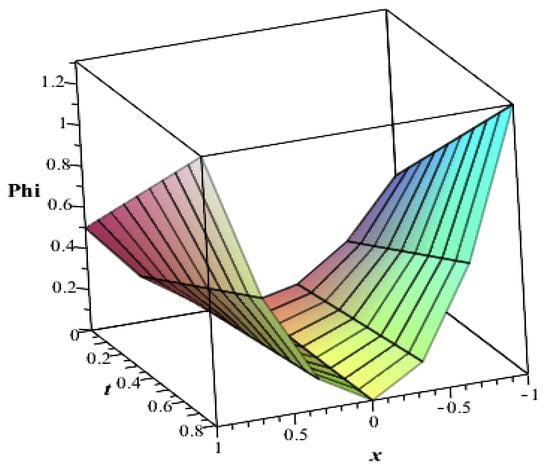
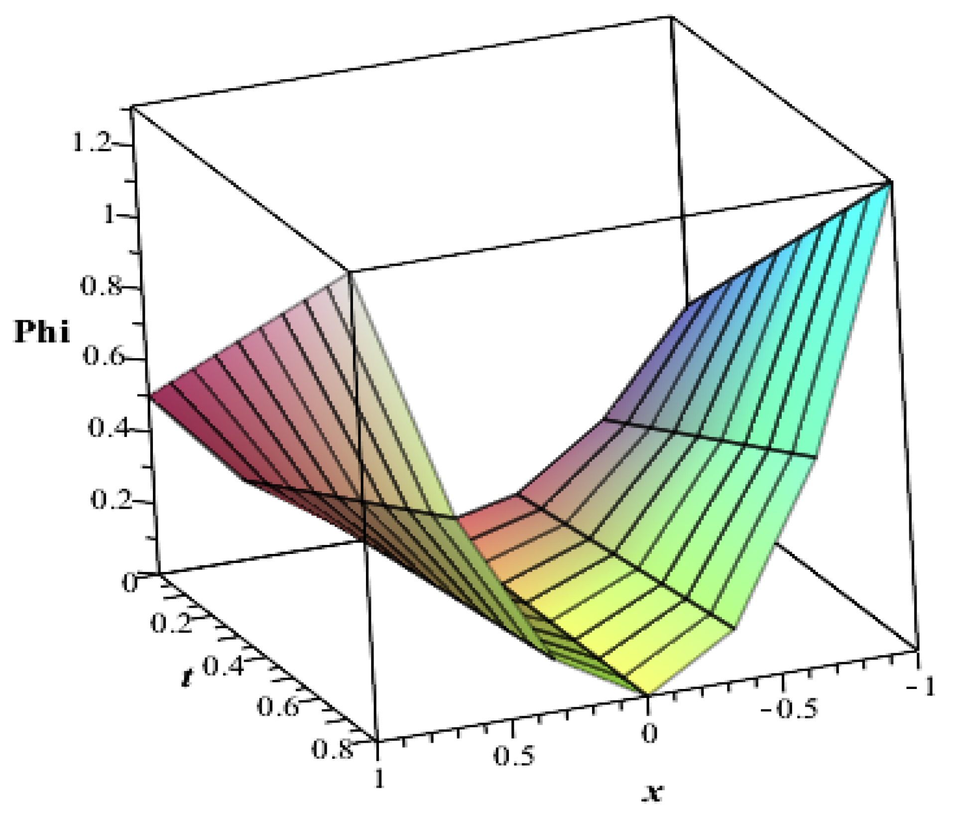
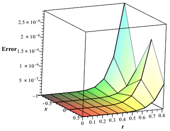
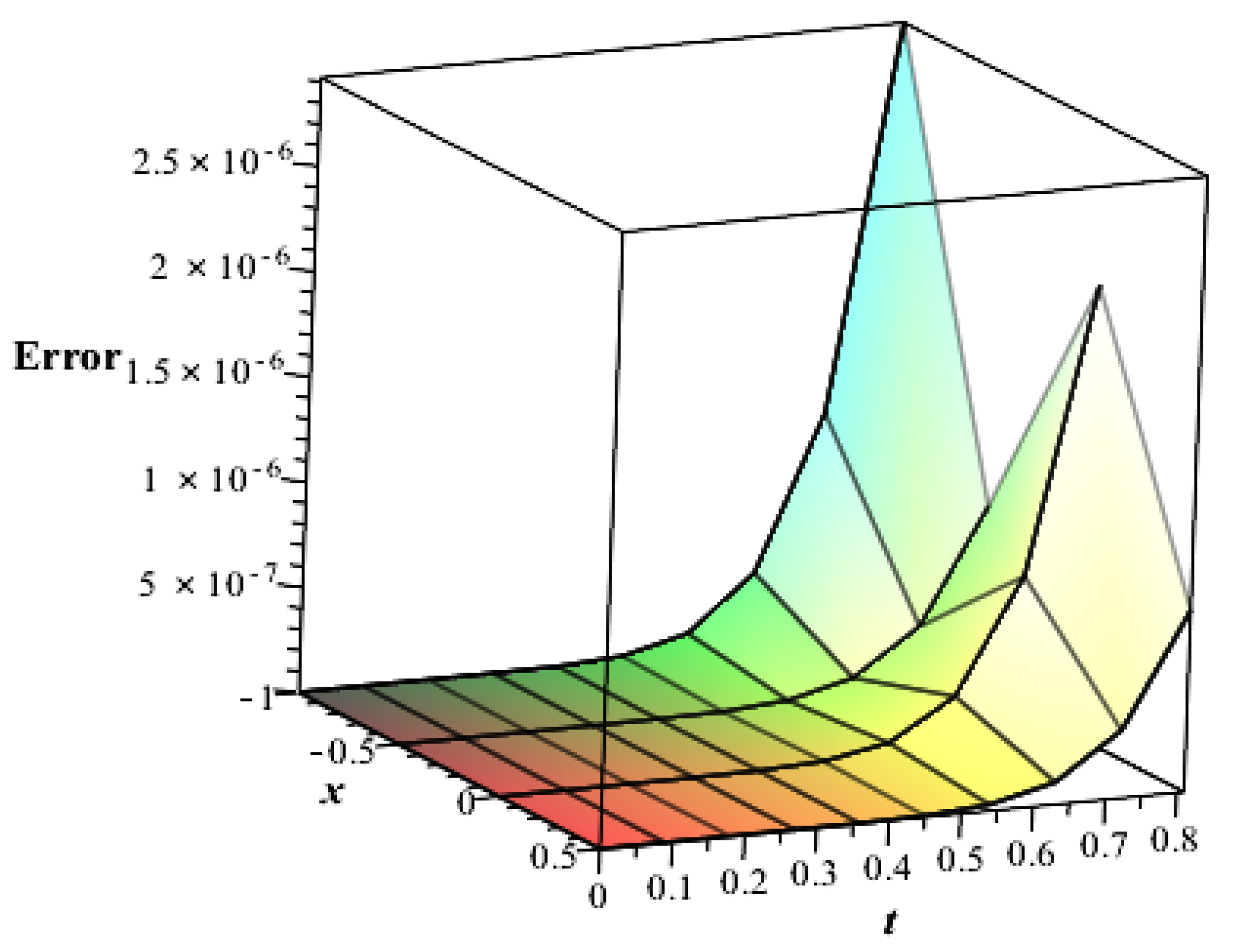
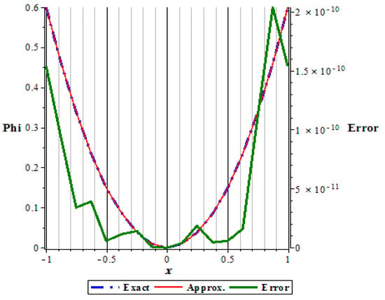
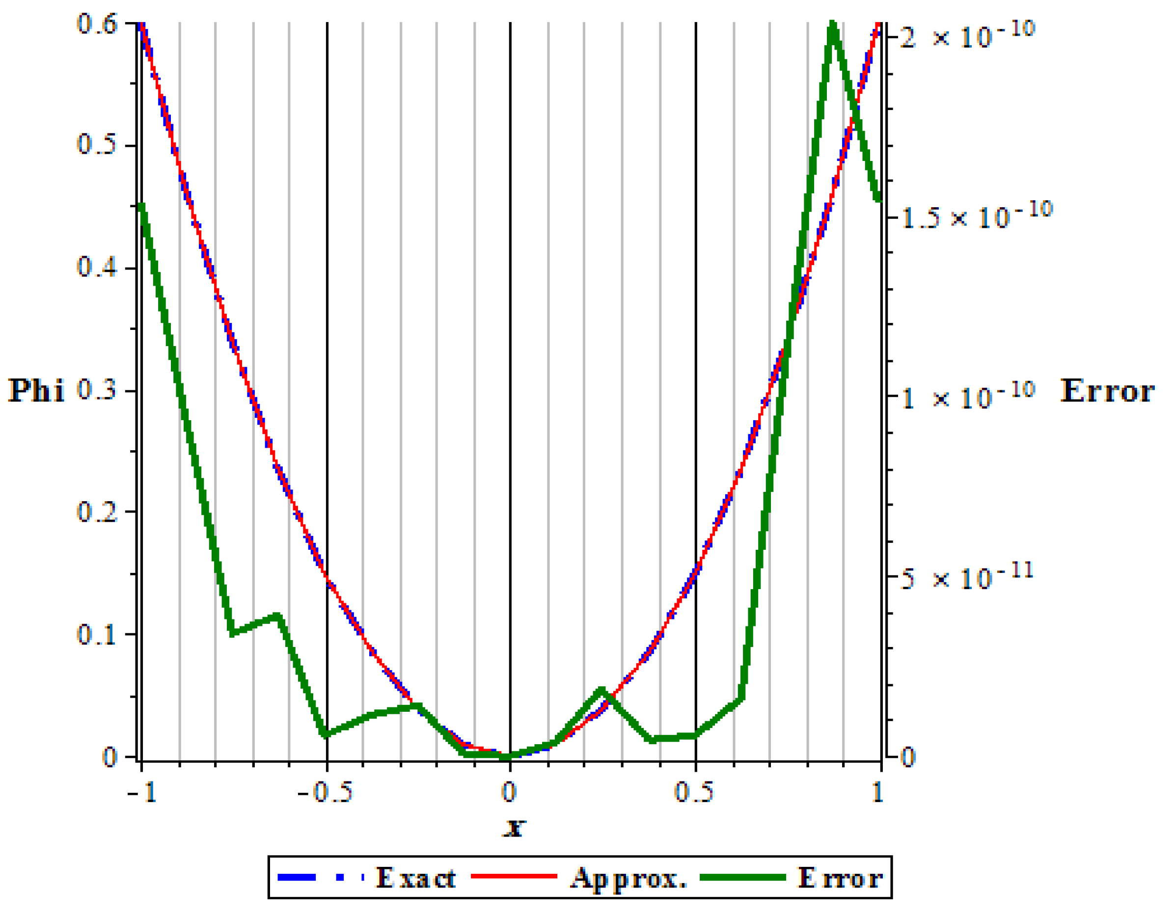
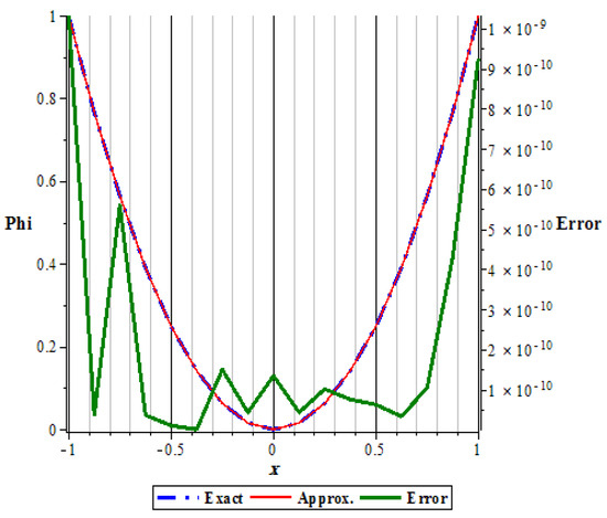
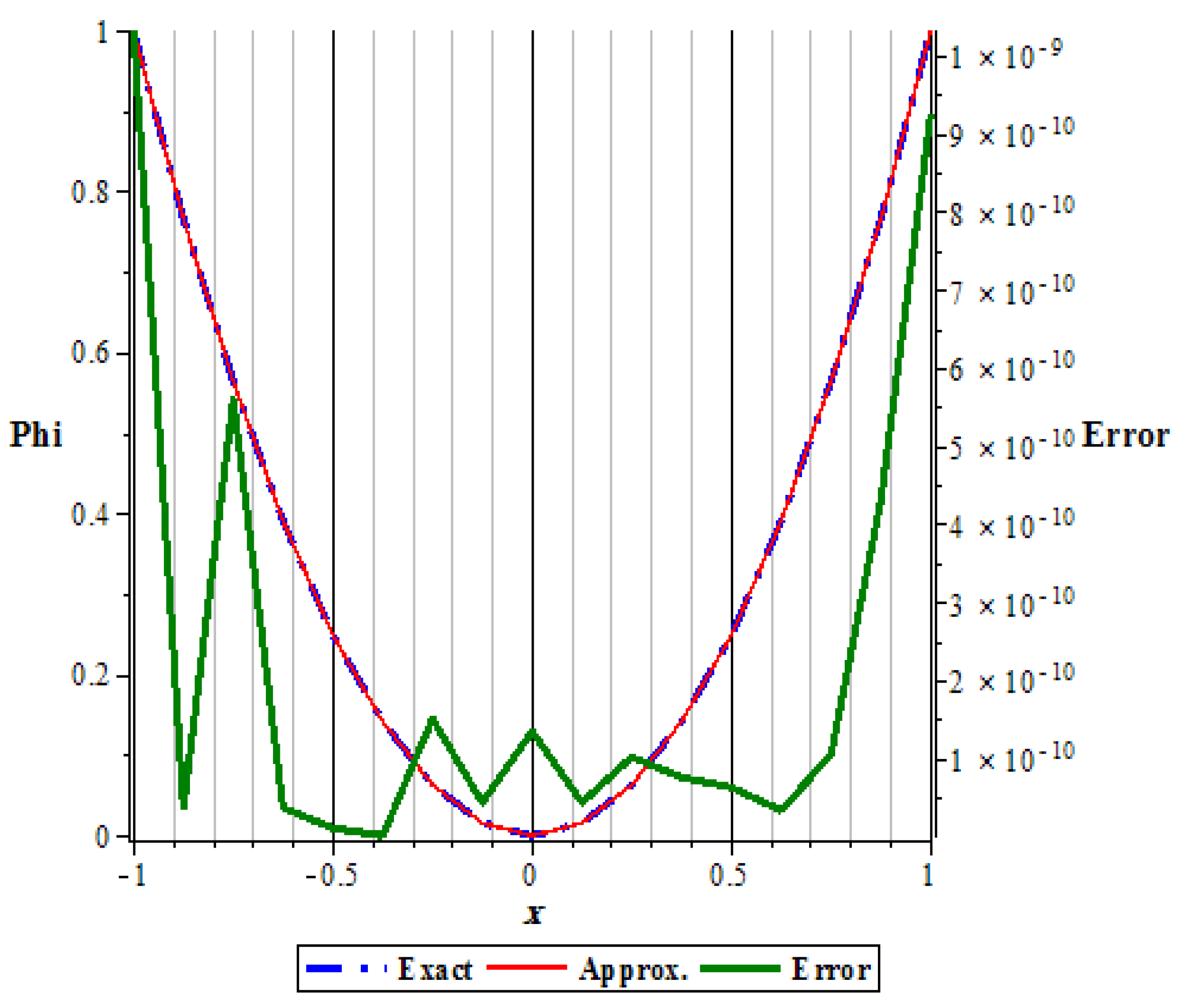
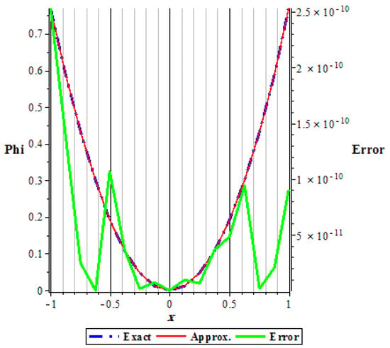
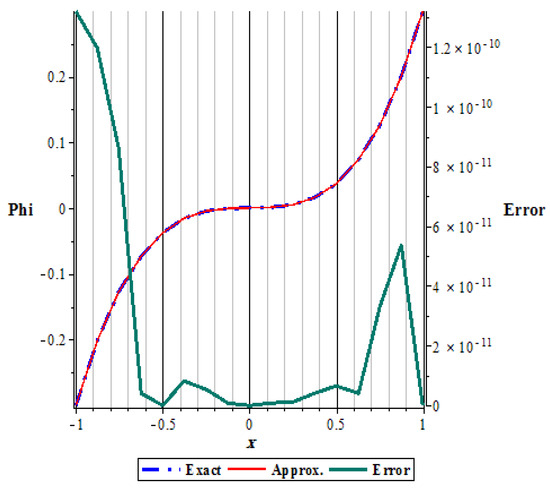
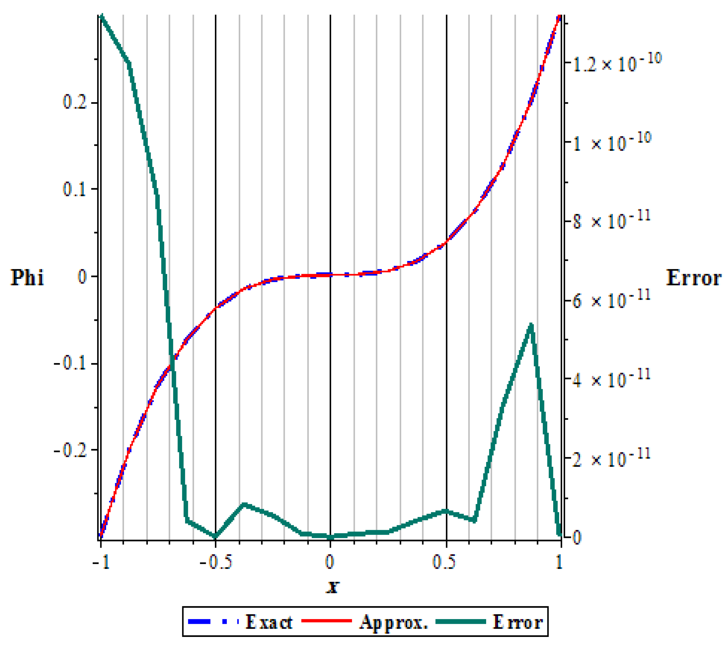
The absolute errors in case (i) with some values of $x\in \left[-1, 1\right]$ are shown in

Table 1. The error for different.$\nu .$ of the approximate solution in case (i) in which $X\left(x\right)=[0.5625, 0.2500, 0.0625, 0.2500, 0.5625]$ at the given points above reduced to ${10}^{-5}$.

T	X	$\mathbf{Error} \left(\mathit{\nu }=0.01\right)$	$\mathbf{Error} \left(\mathit{\nu }=0.47\right)$
0.0	–0.75	2.000 × 10−10	2.000 × 10−10
	−0.5	1.000 × 10−10	1.000 × 10−10
	0.25	1.000 × 10−11	1.000 × 10−11
	0.5	0.000	0.000
	0.75	0.000	0.000
0.1	−0.75	0.000	0.000
	−0.5	1.000 × 10−10	1.000 × 10−10
	0.25	1.000 × 10−11	1.000 × 10−11
	0.5	1.000 × 10−10	1.000 × 10−10
	0.75	0.000	0.000
0.5	−0.75	8.000 × 10−10	1.200 × 10−9
	−0.5	9.000 × 10−10	1.300 × 10−9
	0.25	8.400 × 10−10	1.400 × 10−10
	0.5	9.000 × 10−10	1.200 × 10−9
	0.75	9.000 × 10−10	1.200 × 10−9
0.9	−0.75	8.770 × 10−8	1.294 × 10−7
	−0.5	8.460 × 10−8	1.326 × 10−7
	0.25	8.533 × 10−8	1.337 × 10−8
	0.5	8.480 × 10−8	1.327 × 10−7
	0.75	8.750 × 10−8	1.293 × 10−7

and the approximate solution $\phi \left(x,t\right)=(\mathrm{t}+0.5)x^2$ is represented by Figure 1 while the errors for different T are shown by Figure 2, Figure 3, Figure 4, Figure 5 and Figure 6. The errors in case (ii) are shown in

Table 2. The error for different.$\nu .$ of the approximate solution in case (ii).

T	X	$\mathbf{Error} \left(\mathit{\nu } = 0.01\right)$	$\mathbf{Error} \left(\mathit{\nu } = 0.47\right)$
0.0	–0.75	0.000	0.000
	−0.5	1.000 × 10−10	1.000 × 10−10
	0.25	0.000	0.000
	0.5	0.000	0.000
	0.75	1.000 × 10−10	1.000 × 10−10
0.1	−0.75	2.000 × 10−10	2.000 × 10−10
	−0.5	1.000 × 10−10	1.000 × 10−10
	0.25	1.000 × 10−11	1.000 × 10−11
	0.5	0.000	0.000
	0.75	2.000 × 10−10	2.000 × 10–10
0.5	−0.75	9.000 × 10−10	1.300 × 10−9
	−0.5	9.000 × 10−10	1.400 × 10−9
	0.25	8.400 × 10−10	1.300 × 10−10
	0.5	1.000 × 10−9	1.200 × 10−9
	0.75	9.000 × 10−10	1.300 × 10−9
0.9	−0.75	8.770 × 10−8	1.293 × 10−7
	−0.5	8.460 × 10−8	1.326 × 10−7
	0.25	8.532 × 10−8	1.337 × 10−8
	0.5	8.480 × 10−8	1.326 × 10−7
	0.75	8.740 × 10−8	1.293 × 10−7

and Figure 7 and Figure 8.

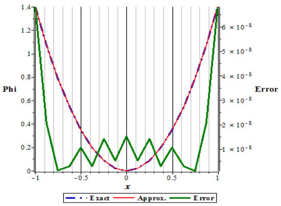
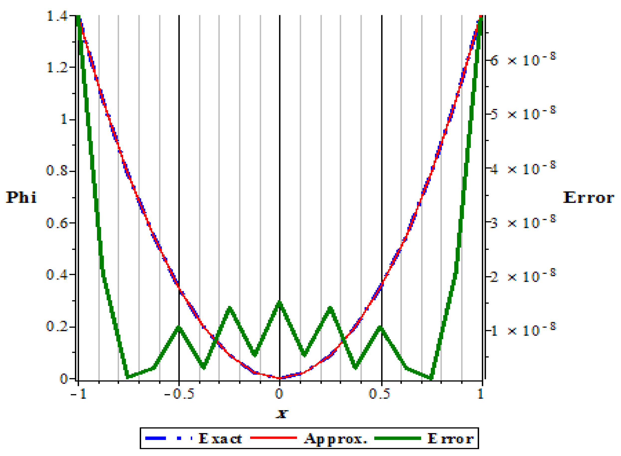
The error increases with time and decreases by increasing the number of iterations, see Figure 3, Figure 4, Figure 5, Figure 6, Figure 7 and Figure 8.

Example 2.

Consider Equation (41) with $k\left(\left|x-y\right|\right)=\mathit{ln}\left|x-y\right|$, we obtain

$$\begin{gathered} \frac{{0.03}^{1.75}}{\mathsf{\Gamma }\left(2.75\right)}\left(\phi \left(x,t\right)-0.5x^2\right)-\frac{{0.03}^{1.75}x}{\mathsf{\Gamma }\left(2.75\right)\Gamma \left(0.75\right)}{\int }_0^t{\left(t-\tau \right)}^{-0.25}d\tau \\ +\frac{{0.03}^{0.75}}{\mathsf{\Gamma }\left(1.75\right)}{\int }_0^t\phi \left(x,\tau \right)d\tau +\frac{1}{\mathsf{\Gamma }\left(0.75\right)}{\int }_0^t{\left(t-\tau \right)}^{\alpha }\phi \left(x,\tau \right)d\tau \\ -\frac{\lambda }{2\Gamma \left(0.75\right)}{\int }_0^t{\int }_{-1}^1{\left(t-\tau \right)}^{1.75}\ln \left|x-y\right|{\tau }^3{t}^3{\phi }^2\left(y,\tau \right)dyd\tau \\ =\frac{1}{\mathsf{\Gamma }\left(0.75\right)}{\int }_0^t{\left(t-\tau \right)}^{\alpha }f\left(x,\tau \right)d\tau . \end{gathered}$$

(45)

Here, $f\left(x,t\right)=\left(0.1+\sin t \right)g\left(x\right)$ is given by putting $\phi \left(x,t\right)=X\left(x\right)N\left(t\right),X=x^3,N\left(t\right)=0.3\cos t$ as an exact value.

The rate of errors is evaluated using the following formula: $Rate=\left|{\log }_2\frac{Error\left(2N\right)}{Error\left(N\right)}\right|.$

By increasing N, the error decreases and the rate of convergence is given below, see

Table 3. Convergence rate in both methods with fixed time $T=0.0$.

N	Mean Error	Rate
4	2.4 × 10−10	0.49
8	1.7 × 10−10	0.79
16	9.8 × 10−11	0.16
32	8.8 × 10−11	---

,

Table 4. Convergence rate in both methods with fixed time $T=0.3$.

N	Mean Error	Rate
4	4.8 × 10−10	0.94
8	2.5 × 10−10	1.32
16	1.0 × 10−10	0.12
32	9.2 × 10−11	---

,

Table 5. Convergence rate in both methods with fixed time $T=0.6$.

N	Mean Error	Rate
4	5.8 × 10−8	0.16
8	6.5 × 10−8	3.92
16	4.3 × 10−9	2.10
32	1.0 × 10−9	---

and

Table 6. Convergence rate in both methods with fixed time $T=0.9$.

N	Mean Error	Rate
4	8.9 × 10−7	2.89
8	1.2 × 10−7	3.79
16	8.7 × 10−9	1.92
32	2.3 × 10−9	---

.

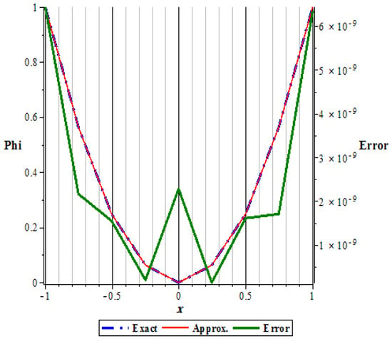
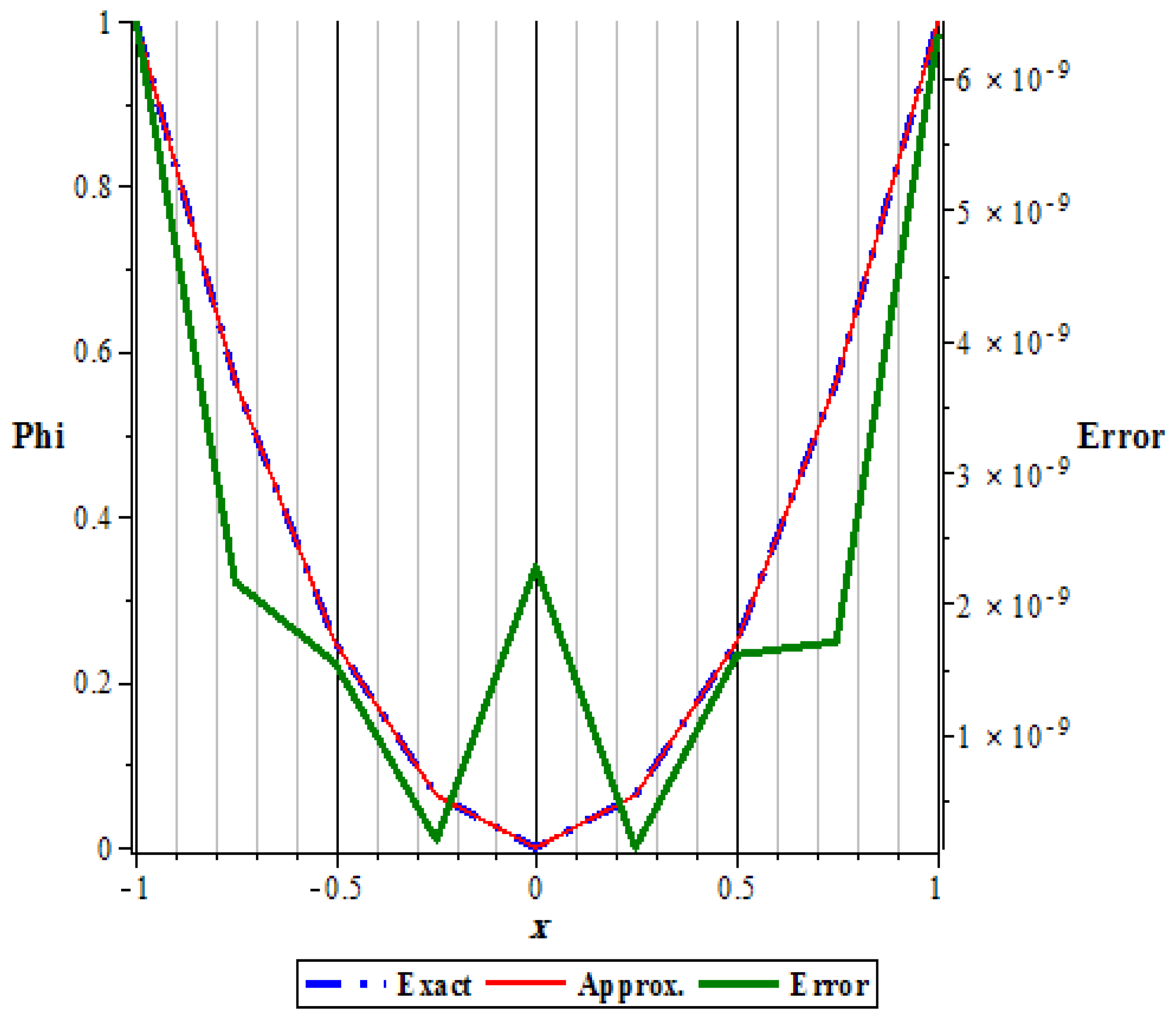
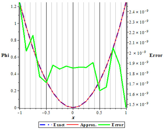
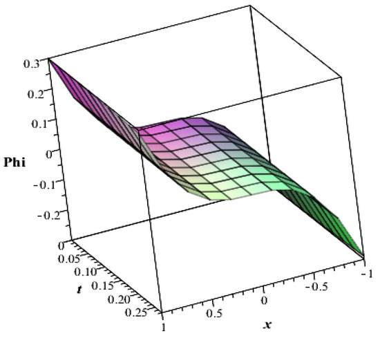
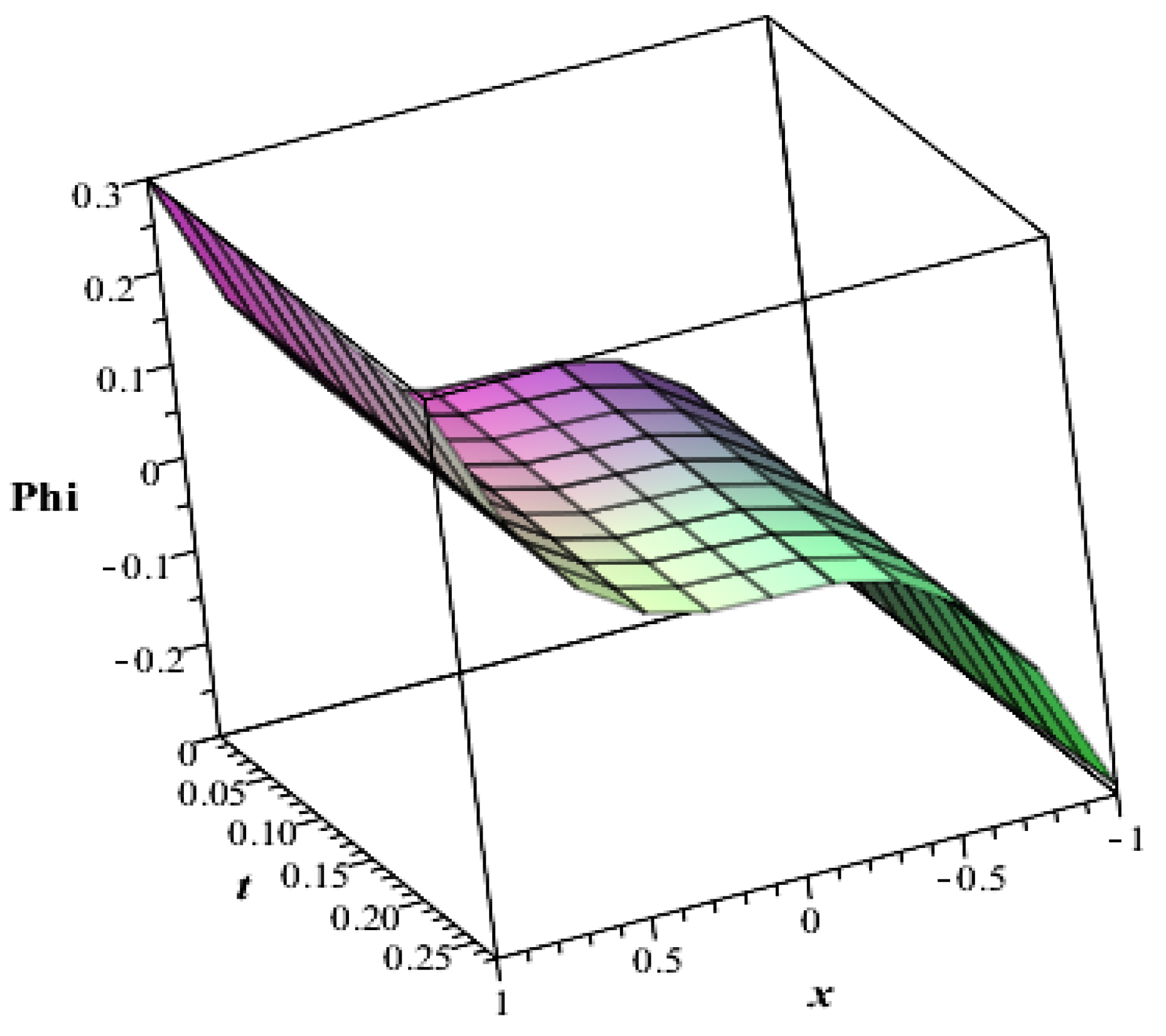
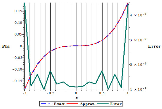
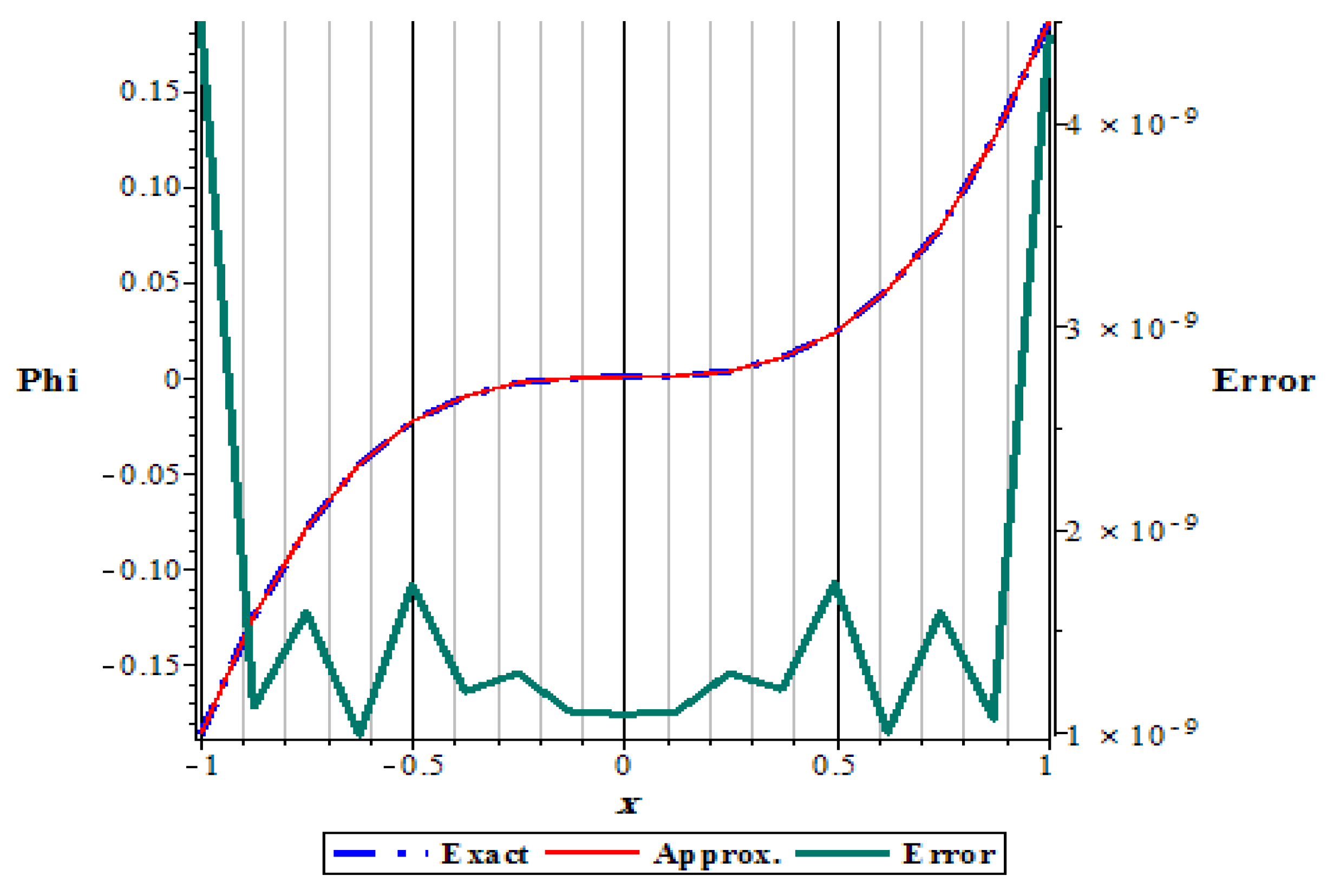
The approximate solution is shown in Figure 9, and the absolute errors with different time are shown in Figure 10 and Figure 11.

11. Conclusions

Fractional calculus has proved to be a valuable tool for modeling and analyzing numerous phenomena with non-local and memory-dependent characteristics. In this research, we focus on the study of fractional nonlinear integral equations with a time-dependent coefficient using the separation technique method. By employing this approach, we aim to transform the integral equation into a class of integral equations with coefficients on time, which can be subsequently solved using the Nystrom method. From the previous work and discussion, we can establish the following:

• The separation technique method is a powerful mathematical tool that allows us to transform fractional nonlinear integral equations with time-dependent coefficients into a class of integral equations with coefficients on time only. This technique simplifies the problem by separating the time-dependent part from the integral part, enabling us to handle the integral equations more efficiently.
• We present the Nystrom method as a numerical scheme to solve the sub-equations derived from the separation process. The Nystrom method efficiently discretizes the integral equation using a set of points and exploits the smoothness of the kernel functions to achieve high accuracy and computational efficiency. We discuss the convergence analysis and error estimates associated with the Nystrom method for the proposed fractional integral equations.
• In the Carleman kernel, when decreasing $\nu$, the solution becomes better, see Table 1.
• The error increases with time, see Figure 3, Figure 4, Figure 5, Figure 6, Figure 7 and Figure 8.
• The error decreases by increasing the number of iterations, see Table 3, Table 4, Table 5 and Table 6.
• CPU Time for Intel^® Core(TM) i7 CPU M 620 @ 2.67 GHz (64-bit Operating system) in example 2 takes the following:

N	Time in Seconds	Memory
4	10.4	59 M.
8	14.34	219.19 M.
16	34.32	215.9 M.

• The error is the same to an extreme degree between positive and negative values for x in the region of integration. We note that the maximum error occurs at the ends of x values while it takes the minimum in the middle, see Figure 2.

12. Future Work

We will attempt to solve Equation (1) as a phase-lag problem with a history memory function in the sense of general form of fractional calculus and differ between the three following cases of time: terrestrial ($T<1$), eternal ($T>1$), and isthmus lives ($T=1$).

References

- Herrmann, R. Fractional Calculus: An Introduction for Physicists; World Scientific: Singapore, 2014. [Google Scholar]
- Oyedepo, T.; Taiwo, O.A. Numerical Studies for Solving Linear Fractional Integro-differential Equations Based on Constructed Orthogonal Polynomials. ATBU J. Sci. Technol. Educ. 2019, 7, 1–13. [Google Scholar]
- Mohammed, O.H.; Altaie, S.A. Approximate solution of Fractional Integro-Differential Equations by using Bernstein polynomials. Eng. Technol. J. 2012, 30, 1362–1373. [Google Scholar] [CrossRef] [Scilit]
- Daşcıoğlu, A.; Bayram, D.V. Solving Fractional Fredholm Integro-Differential Equations by Laguerre Polynomials. Sains Malays. 2019, 48, 251–257. [Google Scholar] [CrossRef] [Scilit]
- Mohammed, D.S. Numerical solution of Fractional Integro-differential Equations by least squares method and shifted Chebyshev polynomial. Comp. Methods Eng. Sci. 2014, 2014, 431965. [Google Scholar] [CrossRef] [Scilit]
- Mahdy, A.M.S.; Mohamed, E.M.H.; Marai, G.M.A. Numerical solution of fractional integro-differential Equations by least squares method and shifted Chebyshev polynomials of the third kind method. Theor. Math. Appl. 2016, 6, 87–101. [Google Scholar]
- Nanware, J.A.; Goud, P.M.; Holambe, T.L. Solution of Fractional Integro-differential Equations by Bernstein Polynomials. Malaya. J. Mat. 2020, 1, 581–586. [Google Scholar] [CrossRef] [Scilit]
- Oyedepo, T.; Taiwo, O.A.; Adebisi, A.F.; Ishola, C.Y.; Faniyi, O.E. Least Squares Method and Homotopy Perturbation Method for Solving Fractional Integro-Differential Equations. Pac. J. Sci. Technol. 2019, 20, 86–95. [Google Scholar]
- Basseem, M.; Alalyani, A. On the Solution of Quadratic Nonlinear Integral Equation with Different Singular Kernels. Math. Probl. Eng. 2020, 2020, 7856207. [Google Scholar] [CrossRef] [Scilit]
- Katani, R. Numerical solution of the Fredholm integral Equations with a quadrature method. SeMA J. 2018, 76, 271–276. [Google Scholar] [CrossRef] [Scilit]
- Al-Bugami, A.M. Numerical Treating of Mixed Integral Equation Two-Dimensional in Surface Cracks in Finite Layers of Materials. Adv. Math. Phys. 2022, 2022, 3398175. [Google Scholar] [CrossRef] [Scilit]
- Brezinski, C.; Redivo-Zaglia, M. Extrapolation methods for the numerical solution of nonlinear Fredholm integral Equations. J. Integral Equ. Appl. 2019, 31, 29–57. [Google Scholar] [CrossRef] [Scilit]
- Bakhshayesh, S.J. Discontinuous Galerkin Approximations for Volterra Integral Equations of the First Kind with Convolution Kernel. Indian J. Sci. Technol. 2015, 8, 33. [Google Scholar] [CrossRef] [Scilit]
- Alkan, S.; Hatipoglu, V.F. Approximate solutions of Volterra-Fredholm integro-differential Equations of fractional order. Tbil. Math. J. 2017, 10, 1–13. [Google Scholar] [CrossRef] [Scilit]
- Mosa, G.A.; Abdou, M.A.; Gawish, F.A.; Abdalla, M.H. On the behavior solutions of fractional and partial integro differential heat Equations and its numerical solutions. Math. Slovak 2022, 72, 397–410. [Google Scholar] [CrossRef] [Scilit]
- Jebreen, H.B.; Dassios, I. On the Wavelet Collocation Method for Solving Fractional Fredholm Integro-Differential Equations. Mathematics 2022, 10, 1272. [Google Scholar] [CrossRef] [Scilit]
- Akram, T.; Ali, Z.; Rabiei, F.; Shah, K.; Kumam, P. A Numerical Study of Nonlinear Fractional Order Partial Integro-Differential Equation with a Weakly Singular Kernel. Fractal Fract. 2021, 5, 85. [Google Scholar] [CrossRef] [Scilit]
- Abdelkawy, M.A.; Amin, A.Z.M.; Lopes, A.M.; Hashim, I.; Babatin, M.M. Shifted Fractional-Order Jacobi Collocation Method for Solving Variable-Order Fractional Integro-Differential. Fractal Fract. 2021, 6, 19. [Google Scholar] [CrossRef] [Scilit]
- Khalil, H. The use of Jacobi polynomials in the numerical solution of coupled system of fractional differential Equation. Int. J. Comput. Math. 2014, 92, 1452–1472. [Google Scholar] [CrossRef] [Scilit]
- Abdou, M.A. On the solution of linear and nonlinear integral Equation. J. App. Math. Comp. 2014, 146, 857–871. [Google Scholar] [CrossRef] [Scilit]
- Abdou, M.A.; Raad, S.A. Nonlocal solution of a nonlinear partial differential Equation and its equivalent of nonlinear integral Equation. Inter. J. Comp. Math. 2014, 92, 1452–1472. [Google Scholar] [CrossRef] [Scilit]
- Mosal, G.A.; Abdou, M.A.; Rahby, A.S. Numerical solutions for nonlinear Volterra-Fredholm integral equations of the second kind with a phase lag. AIMS Math 2021, 6, 8525–8543. [Google Scholar] [CrossRef] [Scilit]
Disclaimer/Publisher’s Note: The statements, opinions and data contained in all publications are solely those of the individual author(s) and contributor(s) and not of MDPI and/or the editor(s). MDPI and/or the editor(s) disclaim responsibility for any injury to people or property resulting from any ideas, methods, instructions or products referred to in the content. |
© 2023 by the authors. Licensee MDPI, Basel, Switzerland. This article is an open access article distributed under the terms and conditions of the Creative Commons Attribution (CC BY) license (https://creativecommons.org/licenses/by/4.0/).