Fractional Control of a Class of Underdamped Fractional Systems with Time Delay—Application to a Teleoperated Robot with a Flexible Link

Abstract

This work addresses the robust control of processes of the form $G\left(s\right)=K·e^{-\tau ·s}/(1+T·s^{\lambda })$ with $1<\lambda \le 2$. A new method for tuning fractional-order $PI$ and $PD$ controllers is developed. The stability is assessed based on the frequency domain tuning of the regulators to control such delayed fractional-order underdamped processes. In order to analyze the closed-loop stability and robustness, the new concept of Robust High-Frequency Condition is introduced. The analysis based on that demonstrates that each controller has a different region of feasible frequency specifications, and, in all cases, they depend on their fractional integral or derivative actions. Finally, an application example, the position control of a teleoperated manipulator with a flexible link, is presented. Simulations and experiments illustrate that the region of feasible frequency specifications defined at low and high frequencies allows us to obtain robust controllers that fulfill frequency requirements.

1. Introduction

Fractional calculus has indeed experienced significant advancements in theory, methods, and applications over the past few decades. It provides a powerful mathematical framework for describing and analyzing systems with memory effects and hereditary properties. Using the fractional-order framework in modeling is crucial for describing real-world applications such as in the field of forecasting and predictions [1], or physical domain such as modeling the nonlinear water waves that integer-order models cannot accurately represent [2]. Thereby, unlike traditional integer-order modeling, fractional order is important because it offers a more accurate and versatile way to describe various real-world phenomena and systems. The development of fractional calculus has led to a deeper understanding of complex systems exhibiting non-local and non-Markovian behavior. It has found applications in diverse fields such as physics [3], engineering [4], biology [5], finance [6], signal processing [7], and control systems [8]. Viscoelastic materials are a class of materials that exhibit mechanical behavior between pure elasticity and pure viscosity. They possess both elastic and viscous characteristics, resulting in unique mechanical properties that have found wide applications in various fields [9]. Fractional calculus has been successfully employed in modeling the constitutive relations of viscoelastic behaviors [10,11]. Several fractional-order viscoelastic models have been established and validated by experimental data, such as the fractional Poynting-Thomson model [12], the fractional Maxwell model [11], and the fractional Kelvin-Voigt model [13].

In addition, the fractional-order $PID$ (Proportional-Integral-Derivative) controller was defined as the generalization of the classical $PID$ controller that incorporates fractional calculus principles. It utilizes fractional derivatives and integrals to capture memory effects and hereditary properties, providing improved control performance in systems with non-local and non-Markovian behaviors. The design of such a controller based on frequency specifications is a fairly broadly used approach [14]. While the traditional phase margin, gain margin, gain crossover frequency, and phase crossover frequency are commonly used in the design of classical $PID$ controllers, their application to fractional-order $PID$ controllers is less straightforward [15]. This is because fractional-order $PID$ controllers introduce additional complexity due to the fractional calculus operators involved. Those specifications have a twofold purpose in the design of control systems, including both classical and fractional-order $PID$ controllers. Frequency specifications relate to both time-domain performance and robustness considerations. An interesting feature of these techniques is, therefore, that they allow the design of the dynamic response of closed-loop control systems, and also permit the design of robustness properties for the controller [16]. Meanwhile, achieving robustness properties in both classical and fractional-order $PID$ controllers becomes more complex when using time domain or Laplace domain-based design techniques than when using frequency domain approaches [17].

The presence of time delay in controlled systems can produce a detrimental effect on the closed-loop performance if it is not considered during the controller design process. In the worst-case scenario, it can even result in instability. For example, time delays can arise from the physical and operational characteristics of a system. Friction-induced delays [18,19] and the nature of certain manufacturing processes such as milling [20] or metal cutting [21] can contribute to these delays. Delays can also be attributed to the mechatronic instrumentation used in real-time experimental systems, where sensors, actuators, and communication networks serve as the primary sources of such delays [22]. Over the years, numerous prominent researchers have addressed this issue by proposing various control solutions. These include integer and fractional-order $PID$ control [23], model predictive control [24], Smith predictor [25,26], communication disturbance observer [27,28], sliding mode control [29], and switching control [30].

From the literature, one can notice that the control of delayed fractional-order monotonic systems has received more investigation and attention than the delayed fractional-order underdamped systems. This is principally due to the complexity of underdamped systems, which exhibit an oscillatory behavior that generally is more complex to analyze and control [31]. The dominance of delayed monotonic systems in applications is another reason for giving them more attention. Those systems exhibit steady-state convergence without oscillations and are more prevalent in many practical applications [32]. In this sense, we study a kind of delayed, underdamped system in this paper.

On the other hand, Ref. [33] proposed a new method for non-integer order integration based on a Multi-layer Perceptron modelization, which allows for an easy circuit design and a wide range of integration orders. Later, Caponetto discussed the design of an auto-tuning fractional-order proportional-integral-derivative (PID) controller and its implementation on a hardware-in-the-loop simulator for real-time control of unknown plants [34]. The proposed procedure is applicable to systems with delay and order greater than one, provided that specifications on cross-over frequency and phase margin are available.

In this study, we focus on the $P{I}^{\alpha }$ and $P{D}^{\mu }$ controllers with the aim of deriving expressions that simplify their design process for the case of underdamped fractional-order delayed systems with a single oscillation mode. The objective is to design controllers that fulfill either: (a) specific frequency requirements or (b) certain time specifications indirectly by achieving some corresponding frequency specifications. Unlike previous works, we take a different approach by defining the region of attainable frequency specifications rather than the region of stabilizing controllers. Consequently, we obtain sets of reachable frequency specifications instead of sets of controller parameters. We demonstrate that these regions, which are more restrictive than stability regions, not only provide insights into the set of controllers but also offer information on the achievable outcomes with a controller of a given structure. We address these particular structures instead of the general one, which is the $P{I}^{\alpha }{D}^{\mu }$ controller structure, because (1) we are interested in achieving only the three specifications of steady-state error, gain crossover frequency and phase margin for the nominal plant, which can be achieved—in principle—by the proposed structures, that have only three parameters to be tuned, (2) the $P{I}^{\alpha }{D}^{\mu }$ structure has five parameters to be tuned which makes much more complicated to obtain theorems and analytic functions that approximate the specification regions, such as the ones obtained in this paper, and (3) specification plots and robustness regions that will be expressed in this paper in two or three dimension graphics, cannot be graphically represented in the case of the $P{I}^{\alpha }{D}^{\mu }$ structure because they would require plots of four or five dimensions.

As an application example, we focus on the air table $FLR$ (Flexible Link Robot) located at the University of Castilla-La Mancha. In this particular case, we have deliberately introduced an artificial time delay into the system’s outer loop. The system is subsequently fine-tuned around a specific operating point by utilizing a delayed fractional underdamped model. Following this adjustment, a comparative analysis is conducted to evaluate the performance of $P{I}^{\alpha }$ and $P{D}^{\mu }$ controllers in positioning the payload of the robot.

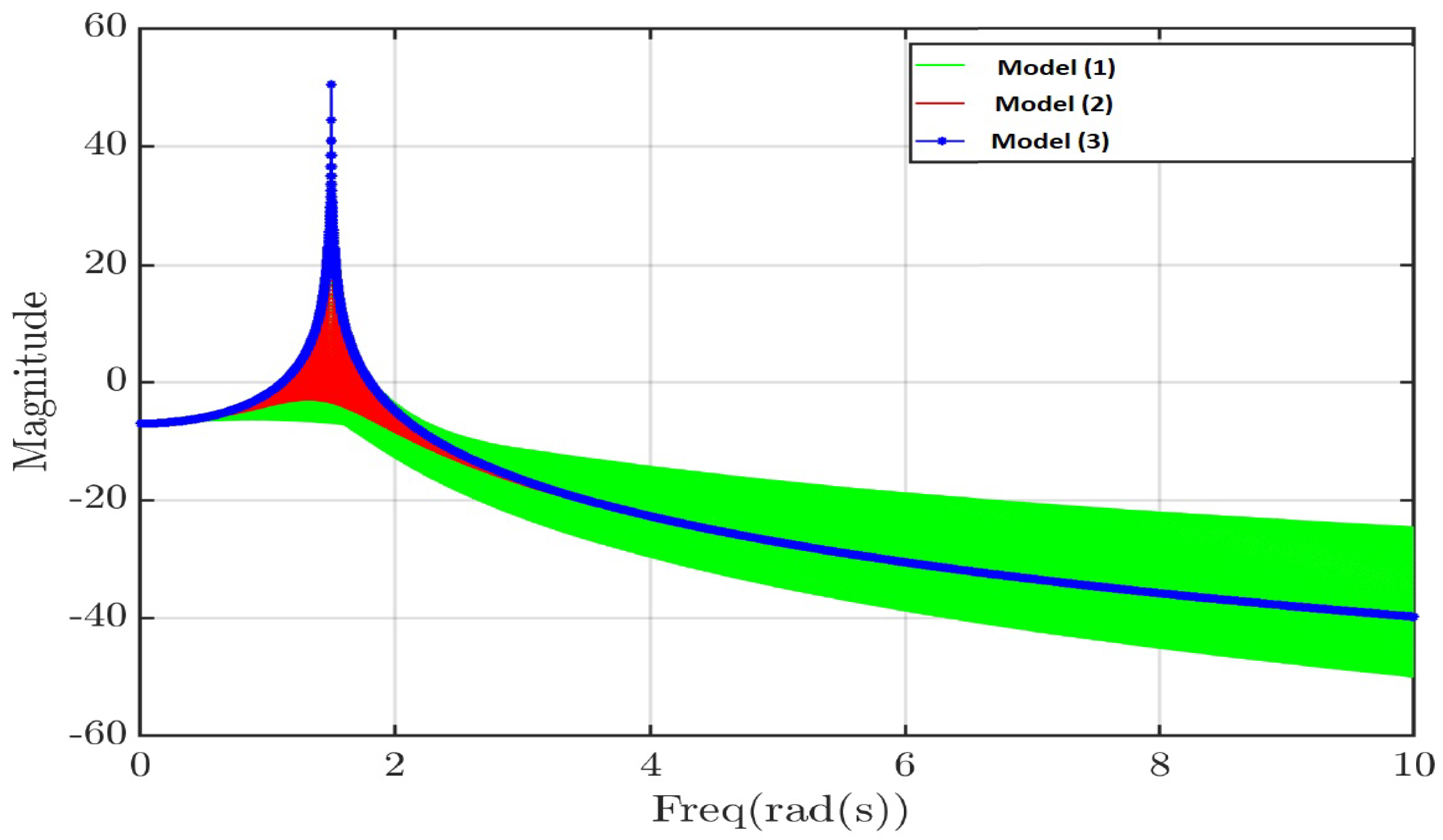
2. Frequency Domain Analysis

In general, the frequency response has to be obtained by the direct evaluation of the irrational-order transfer function of the fractional-order system along the imaginary axis for $s=j\omega$, $\omega \in [0,\infty ]$. However, for the commensurate order systems, we can obtain Bode-like plots. In other words, the frequency response can be obtained by the addition of the individual contributions of the terms of order $\lambda$ resulting from the factorization of the function. For each of these terms, referred to as ${(s^{\lambda }+\sigma )}^{\pm 1}$, the magnitude curve will have a slope that starts at zero and tends to $\pm \lambda ·20dB/dec$ for higher frequencies, and the phase plot will go from 0 to $\pm \lambda ·\pi /2$. If $\lambda$ were a real number, it would give more degrees of freedom than in the case of standard rational models, in which $\lambda$ is integer $\lambda =(1,2,3,\dots )$ [35]. In addition, there will be resonances for $\lambda >1$, which is the case of our considered underdamped system. Figure 1 shows the magnitudes of the frequency responses of fractional-order underdamped, integer-order underdamped, and integer-order undamped systems, whose transfer functions are, respectively:

$$G\left(s\right)=\frac{K}{T·s^{\lambda }+1}·e^{-\tau ·s}$$

(1)

$$G\left(s\right)=\frac{K}{s^2+2·\zeta ·s+{\omega }_0^2}·e^{-\tau ·s}$$

(2)

$$G\left(s\right)=\frac{K}{s^2+{\omega }_0^2}·e^{-\tau ·s}$$

(3)

where

Figure 1. Frequency-responses: Model $\left(1\right)$ vs. Model $\left(2\right)$ vs. Model $\left(3\right)$.

• $K=1$ is the static gain;
• ${\omega }_0$ = 1.64 (rad/s) is the fundamental frequency of vibration of the beam;
• $\zeta \in [0,1]$ is the damping coefficient;
• $T=0.645$ s is the time constant of the model (1), and $\lambda \in \left[12\right]$ is the order of the fractional order model;
• $\tau =0.5$ s is the time delay, which is unique for the three models.

In Figure 1, the green plot represents the magnitude of model (1). It is evident that this model exhibits a wider distribution, particularly in the high-frequency domain, compared to the other two integer models.

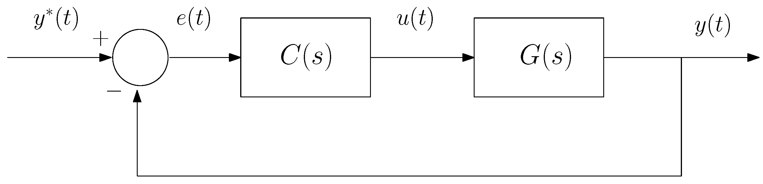
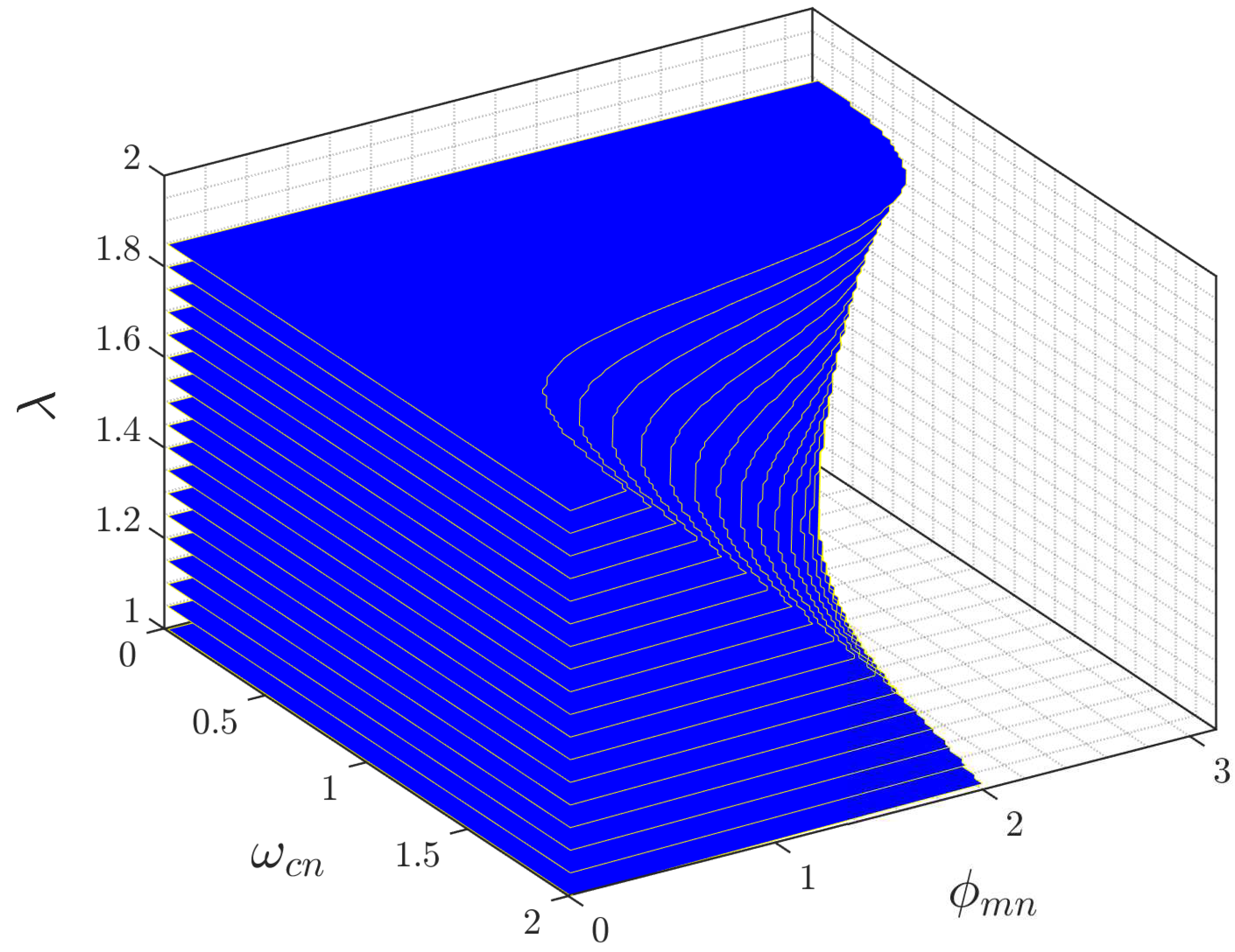
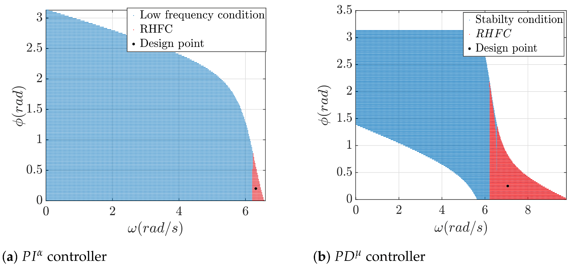
3. Region of Feasible Frequency Specifications: $P{I}^{\alpha }$ Controller

The proposed method focuses on controlling fractional-order delayed processes of the form (1) such that $(1<\lambda ⩽2)$ using fractional order $P{I}^{\alpha }$ controller $(0<\alpha ⩽1)$. The stability and the robustness of the controlled system are studied at low and high-frequency domains. Moreover, for values of $\lambda >1$, the step response of the process is underdamped, and it is stable if $T>0$.

We consider the negative unity feedback control scheme shown in Figure 2. Our aim is to design a control system for the process (4) that verifies certain typical frequency specifications: (a) desired gain crossover frequency, ${\omega }_c$, which is related to the desired nominal speed of the closed loop system response, (b) desired phase margin, ${\varphi }_m$, which provides the desired damping and robustness to changes in time delay and (c) zero steady-state error to a step command, which means that the controller must include an integral term (of integer or fractional order), according to the Final Value Theorem.

Figure 2. Block diagram of the unity feedback control system.

The aim is to develop a general tuning method based on a set of frequency specifications. In order to obtain general results, we carry out a normalization procedure. The time vector t is scaled by $T^{1/\lambda }$ $(t_n=t/T^{1/\lambda })$ and the process output $y\left(t\right)$ is scaled by K $(y_n\left(t\right)=y\left(t\right)/K)$. This yields the new normalized process:

$$G_n\left(s\right)=\frac{1}{s^{\lambda }+1}{e}^{-{\tau }_n·s}$$

(4)

where ${\tau }_n$ is the normalized time delay $({\tau }_n=\tau /T^{\lambda })$. Following the normalization process, it is necessary to normalize the gain crossover frequency by applying the formula ${\omega }_{cn}={\omega }_c{T}^{1/\lambda }$. The phase margin does not change because of the normalization process.

The new normalized specifications $({\omega }_{cn},{\varphi }_m)$ and the zero steady error to step commands can then be attained by using a normalized controller $C_n\left(s\right)$ with a pole at the origin of fractional or integer order and at least two parameters to be tuned. We propose the ideal $P{I}^{\alpha }$ controller characterized by the following transfer function:

$$C_n\left(s\right)=\frac{K_{in}}{s^{\alpha }}+K_{pn}$$

(5)

The condition of having given phase margin ${\varphi }_m$ and gain crossover frequency ${\omega }_{cn}$ can be expressed in a compact form using complex numbers:

$$C_n(j·{\omega }_{cn})·G_n(j·{\omega }_{cn})=-e^{j·{\varphi }_m}$$

(6)

Let us denote $Z_r=\Re \left[-e^{j·{\varphi }_m}/G_n(j·{\omega }_{cn})\right]$ and $Z_i=\Im \left[-e^{j·{\varphi }_m}/G_n(j·{\omega }_{cn})\right]$, where ℜ and ℑ are, respectively, the real and imaginary parts of a complex number. Then the controller can be tuned using Equation (6):

$$C_n(j·{\omega }_{cn})=Z_r+j{Z}_i$$

(7)

Operating $-e^{j·{\varphi }_m}/G_n(j·{\omega }_{cn})$ yields:

$$Z_r=-cos({\varphi }_m+{\tau }_n·{\omega }_{cn})·\left({\omega }_{cn}^{\lambda }·cos\left(\frac{\lambda ·\pi }{2}\right)+1\right)+{\omega }_{cn}^{\lambda }·sin({\varphi }_m+{\tau }_n·{\omega }_{cn})·sin\left(\frac{\lambda ·\pi }{2}\right)$$

(8)

$$Z_i=-{\omega }_{cn}^{\lambda }·cos({\varphi }_m+{\tau }_n·{\omega }_{cn})·sin\left(\frac{\lambda ·\pi }{2}\right)-\left({\omega }_{cn}^{\lambda }·cos\left(\frac{\lambda ·\pi }{2}\right)+1\right)·sin({\varphi }_m+{\tau }_n·{\omega }_{cn})$$

(9)

The normalized time delay ${\tau }_n$ as it appears in the above expressions is always linked in the same manner to ${\varphi }_m$. Let us then define the normalized phase margin:

$${\varphi }_{mn}={\varphi }_m+{\tau }_n·{\omega }_{cn}$$

(10)

Expressions (8) and (9) become:

$$Z_r=-cos\left({\varphi }_{mn}\right)·\left({\omega }_{cn}^{\lambda }·cos\left(\frac{\lambda ·\pi }{2}\right)+1\right)+{\omega }_{cn}^{\lambda }·sin\left({\varphi }_{mn}\right)·sin\left(\frac{\lambda ·\pi }{2}\right)$$

(11)

$$Z_i=-{\omega }_{cn}^{\lambda }·cos\left({\varphi }_{mn}\right)·sin\left(\frac{\lambda ·\pi }{2}\right)-\left({\omega }_{cn}^{\lambda }·cos\left(\frac{\lambda ·\pi }{2}\right)+1\right)·sin\left({\varphi }_{mn}\right)$$

(12)

Since the magnitude Bode plot of $G_n\left(s\right)·C_n\left(s\right)$ is independent of the time delay of the process, the gain crossover frequency is independent of the value of the time delay. However, the time delay shifts the Bode phase plot, which is the reason for the previous phase margin normalization. Expressions (8), (9), (11) and (12) suggest that there are two manners to design the controller $C_n\left(s\right)$:

(a):

The controller must fulfill specifications $({\varphi }_m,{\omega }_{cn})$ with the process $G_n\left(s\right)$ of (4).

(b):

The controller must fulfill specifications $({\varphi }_{mn},{\omega }_{cn})$ with the process $G_n^{*}\left(s\right)$:

$$G_n^{*}\left(s\right)=\frac{1}{s^{\lambda }+1}$$

(13)

For the sake of simplicity, we decided to use procedure (b) considering process (13) and the normalized phase margin defined in (10), and taking into account the real phase margin, the normalized delay, and the normalized gain crossover frequency. Accordingly, the real controller is obtained from the normalized one as

$$C\left(s\right)=\frac{1}{K}{C}_n\left(s^{*}\right){|}_{s^{*}=s{T}^{\frac{1}{\lambda }}}$$

(14)

For the sake of simplicity, from now on we will use s instead of $s^{*}$ in $C_n\left(s^{*}\right)$. Substituting Expressions (11) and (12) in Equation (7), the parameters of the fractional order controller can be determined in function of the system characteristics, the normalized phase margin, and the normalized gain crossover frequency:

$$K_{in}=\frac{{\omega }_{cn}^{\alpha }}{sin(\alpha ·\pi /2)}·\left[{\omega }_{cn}^{\lambda }·sin\left({\varphi }_{mn}+\frac{\lambda ·\pi }{2}\right)+sin\left({\varphi }_{mn}\right)\right]$$

(15)

$$K_{pn}=\frac{-1}{sin(\alpha ·\pi /2)}·\left[{\omega }_{cn}^{\lambda }·sin\left({\varphi }_{mn}+\frac{(\lambda +\alpha )·\pi }{2}\right)+sin({\varphi }_{mn}+\frac{\alpha ·\pi }{2})\right]$$

(16)

It is obtained from (10) that ${\varphi }_m={\varphi }_{mn}-{\tau }_n·{\omega }_{cn}$, which shows that the phase margin that can be obtained diminishes as ${\tau }_n$ and ${\omega }_{cn}$ increase. Accordingly, there is a limit on the time delay for each pair of specifications $({\omega }_{cn},{\varphi }_{mn})$, which is valid for integer order systems too.

$${\tau }_{n,max}=\frac{{\varphi }_{mn}}{{\omega }_{cn}}$$

(17)

3.1. Low Frequency Condition

The Nyquist criterion of stability applied to process (13) with $1<\lambda ⩽2$ using controller (5) imposes that the plot must not encircle the limit point of stability $(-1,0)$. Since $C_n\left(s\right)·G_n^{*}\left(s\right)$ exhibits a pole at the origin of order equal to $\alpha$, this implies that:

$$\underset{\omega \to 0^{+}}{lim}{C}_n\left(j\omega \right)·G_n^{*}\left(j\omega \right)$$

must be in the third or fourth quadrant of the complex plane. Otherwise, the gain of the integral term of the controller defines an asymptotic behavior of the controller at low frequencies, and it must verify the following condition in order to achieve closed-loop stability:

$$K_{in}>0$$

(18)

3D low frequency region: The three-dimensional region that defines the low-frequency condition for the normalized fractional-order process (13), controlled by a $P{I}^{\alpha }$ controller (5), is presented in Figure 3. The x-axis represents the normalized gain crossover frequency ${\omega }_{cn}$, the y-axis represents the normalized phase margin ${\varphi }_{mn}$, and the z-axis represents the order of the process $\lambda$. The region does not depend on the fractional order $\alpha$, which means that all $P{I}^{\alpha }$ controllers (including the standard $PI$) share the same low-frequency region for a given process.

Figure 3. Low frequency condition for $1<\lambda ⩽2$.

The base of the volume corresponds to the combinations of ${\omega }_{cn}$ and ${\varphi }_{mn}$ that verify the above stability condition at low frequencies, for the lowest order $\lambda$ (slightly higher than 1). The volume starts decreasing its horizontal section, which reaches its minimum at $\lambda =2$.

We refer to this region as the “Low-Frequency Condition Region”, and it is challenging to find analytical formulae that guarantee this condition for the process (13) combined with controllers (5). In this subsection, we have developed a mathematical model that describes this region for all processes where $1<\lambda ⩽2$.

It is challenging to find analytical formulae that guarantee the feasible frequency conditions for process Equation (13) combined with controllers (5) for all the combinations of fractional order operators $\alpha$ and $\lambda$. However, in Theorems 1 and 2, we will develop some useful partial results that fit the curves of the low and robust high-frequency conditions using mathematical models.

Theorem 1. 

The region of frequency specifications that verify (18) for a process $G_n^{*}\left(s\right)$ of the form (13) and a controller $C_n\left(s\right)$ of the form (5) is given by:

1. 

If $\alpha \in (0,2]$, and $\lambda \in (1,1.3]$

$${\varphi }_{mn}<m_1·e^{m_2·{\omega }_{cn}}+m_3$$

(19)

where:

$$m_1=0.008·e^{5.806·\lambda }+0.424·e^{0.598·\lambda }$$

$$m_2=4.4·\lambda +0.4$$

$$m_3=-0.0085·e^{3.377·\lambda }+2.446·e^{-0.049·\lambda }$$

2. 

If $\alpha \in (0,2]$, and $\lambda \in (1.3,2]$,

$${\varphi }_{mn}<\frac{{\sum }_{k=0}^5{a}_k·{\omega }_{cn}^k}{{\omega }_{cn}^6+{\sum }_{k=0}^5{b}_k·{\omega }_{cn}^k}$$

(20)

$$\left\{\begin{array}{c}{a}_0=0.642·e^{3.167·\lambda }-0.591·e^{0.262·\lambda }\\ a_1=6.029·e^{1.649·\lambda }+3.738·e^{-2.01·\lambda }\\ a_2=-0.441·e^{2.9·\lambda }-0.176·e^{1.375·\lambda }\\ a_3=0.004·e^{0.722·\lambda }-1.189·e^{1.11·\lambda }\\ a_4=1.889·e^{4.177·\lambda }+2.203·e^{0.096·\lambda }\\ a_5=9.266·e^{0.133·\lambda }-3.118·e^{1.205·\lambda }\end{array}\right.$$

$$\left\{\begin{array}{c}{b}_0=-6.79·e^{-1.646·\lambda }+0.001·e^{9.060·\lambda }\\ b_1=0.316·e^{4.075·\lambda }+1.142·e^{-6.485·\lambda }\\ b_2=-2.48·e^{-1.074·\lambda }-3.571·e^{-0.55·\lambda }\\ b_3=-1.69·e^{1.168·\lambda }+3.749·e^{1.876·\lambda }\\ b_4=-0.74·e^{-0.161·\lambda }+0.701·e^{4.075·\lambda }\\ b_5=4.397·e^{0.018·\lambda }+0.401·e^{1.754·\lambda }\end{array}\right.$$

Figure 4 represents the adjusted mathematical model of the Low-frequency condition for several values of $\lambda$.

Figure 4. Low frequency region for $1<\lambda ⩽2$.

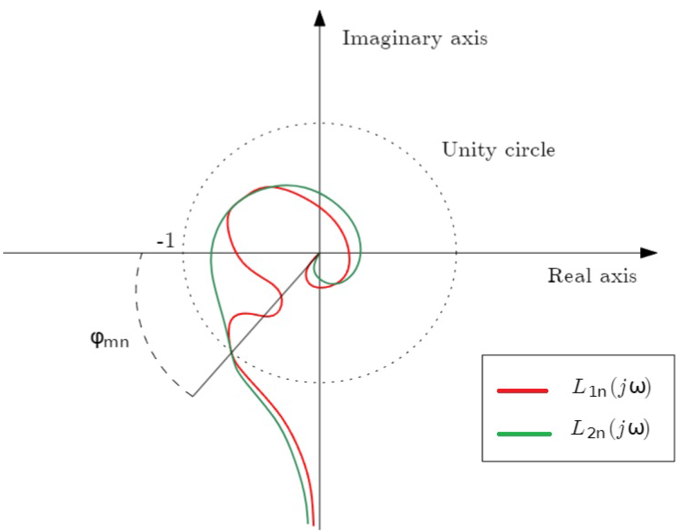
3.2. Robust High-Frequency Condition

3.2.1. Motivation

Figure 5 presents typical Nyquist plots of two systems: $L_{1n}(j·\omega )=C_{1n}(j·\omega )·G_n(j·\omega )$ and $L_{2n}(j·\omega )=C_{2n}(j·\omega )·G_n(j·\omega )$. Both systems satisfy the same phase margin and gain crossover frequency conditions. Moreover, $L_{1n}(j·\omega )$ satisfies the condition

$$\left|L_{1n}(j·\omega )\right|<1,\forall \omega >{\omega }_{cn}$$

(21)

proposed in [17] to guarantee the fulfillment of the previous two frequency specifications. However, $L_{2n}(j·\omega )$ verifies the condition:

$$\frac{d\left|L_{2n}(j·\omega )\right|}{d\omega }<0,\forall \omega >{\omega }_{cn}$$

(22)

Figure 5. Nyquist-diagrams: $L_{1n}\left(j\omega \right)$ vs. $L_{2n}\left(j\omega \right)$.

This last condition, referred to as the ‘Robust High-Frequency Condition: $RHFC$’ not only guarantees the fulfillment of the two frequency specifications but is also more restrictive than the first one.

The plots of Figure 5 demonstrate that the stability of the two systems can be determined by the common phase margin ${\varphi }_{mn}$, which is obtained by evaluating $\pi +\angle L_n\left(j\omega \right)$ at the point on the Nyquist plot where $\left|L_n\left(j\omega \right)\right|=1$ with the highest possible value of $\omega$ (referred to as ${\omega }_{cn}$). A change in the loop gain results in a scaling of the Nyquist plot, which alters the phase margin of both systems. This behavior is illustrated in Figure 6a,b. In the first case in which Condition (21) is verified, the phase margin of $L_{1n}\left(j\omega \right)$ exhibits a significant and sudden reduction due to a small variation in the loop gain. Consequently, there is a substantial increase in the gain crossover frequency. The new phase margin, measured at ${\omega }_{cn1}^{*}$ (where ${\omega }_{cn1}^{*}>{\omega }_{cn1}$), corresponds to a negative value. This sudden instability corresponds to a sharp increase in the gain crossover frequency of the system. However, this phenomenon does not occur in the case in which Condition (22) is verified because the magnitude of $L_{2n}\left(j\omega \right)$ strictly decreases with $\omega$.

Figure 6. Problem-illustration.

3.2.2. Analytical Global Model

Theorem 2. 

The region of frequency specifications that verify the defined $RHFC$ condition for a process $G_n^{*}\left(s\right)$ of the form (13) and a controller $C_n\left(s\right)$ of the form (5) for $\alpha \in \left(01\right]$, $\lambda \in \left(12\right]$ is given by:

1. 

If $\alpha \in (0,0.5]$, and $\lambda \in (1,1.5]$

$${\varphi }_{mn}<{\Sigma }_1·e^{{\Sigma }_2·{\omega }_{cn}}+{\Sigma }_3·e^{{\Sigma }_4·{\omega }_{cn}}$$

(23)

where:

$${\Sigma }_1=0.322·e^{f_1\left(\lambda \right)·\alpha }$$

$$\begin{array}{c}{f}_1\left(\lambda \right)=-14.25·e^{\frac{0.0007-\lambda }{0.0684}}-239.63·e^{\frac{\lambda -0.0924}{0.135}}-1.047·e^{\frac{11.22-\lambda }{2.415}}\end{array}$$

$$\begin{array}{c}{\Sigma }_2=347.18·e^{-9.86·\lambda }-2.14·e^{0.54·\lambda }·e^{\frac{\alpha -0.268·e^{2.441·\lambda }}{7.04·e^{0.039·\lambda }}}\end{array}$$

$$\begin{array}{c}{\Sigma }_3=2.81·e^{-0.91·\lambda }+0.24·e^{1.71·\lambda }·e^{\frac{\alpha -0.0185·e^{-0.51·\lambda }}{0.54·e^{1.083·\lambda }}}\end{array}$$

$$\begin{array}{c}{\Sigma }_4=-1.93·e^{{\left(\frac{0.87-\lambda }{0.49}\right)}^2}·\left(e^{\left(-1.75e^3·\alpha e^{{(-16.77·\lambda )}^2}\right)}+e^{\left(19.9·\alpha e^{{(-2.6·\lambda )}^2}\right)}\right)\end{array}$$

2. 

If $\alpha \in (0.5,1]$, and $\lambda \in (1,1.5]$

$${\varphi }_1<{\varphi }_{mn}<{\varphi }_2$$

(24)

$${\varphi }_1=\sum _{i=1}^4\sum _{j=1}^6{p}_{ij}·{\alpha }^{j-1}·{\omega }_{cn}^{i-1}$$

(25)

$$\left[\begin{array}{c}{p}_{11}\\ p_{12}\\ p_{13}\\ p_{14}\\ p_{15}\\ p_{16}\end{array}\right]=\left[\begin{array}{cccc}-0.945& 1.472& -1.127& -4.056\\ 4.518& -1.014& -193.87& 175.004\\ 9.617& 0.005& -0.015& 0.0172\\ -0.785& 1.105& -0.843& 1.462\\ -4.436& 0.739& 80.818& -122.67\\ 4.858& -0.038& 0.031& -0.063\end{array}\right]·\left[\begin{array}{c}{\lambda }^3\\ {\lambda }^2\\ \lambda \\ 1\end{array}\right]$$

$$\left[\begin{array}{c}{p}_{21}\\ p_{22}\\ p_{23}\\ p_{24}\\ p_{25}\\ p_{26}\end{array}\right]=\left[\begin{array}{cccc}-1.057& 0.509& 0.046& 1.58\\ -12.72& 0.725& 382.07& -234.49\\ -20.42& -0.008& -0.030& -0.030\\ 0.021& 0.333& -0.157& -0.206\\ 1.267& 0.159& -26.36& 13.518\\ -5.97& 0.008& -0.069& 0.035\end{array}\right]·\left[\begin{array}{c}{\lambda }^3\\ {\lambda }^2\\ \lambda \\ 1\end{array}\right]$$

$$\left[\begin{array}{c}{p}_{31}\\ p_{32}\\ p_{33}\\ p_{34}\\ p_{35}\\ p_{36}\end{array}\right]=\left[\begin{array}{cccc}-0.333& 0.293& -0.181& 0.4174\\ 2.2071& -1.7171& -240.8178& 127.0347\\ 3.3305& -0.010& 0.003& 0.007\\ 0.022& -0.378& -0.044& 1.126\\ -8.485& -0.576& 59.70& -23.38\\ 2.080& 0.004& -0.040& -0.021\end{array}\right]·\left[\begin{array}{c}{\lambda }^3\\ {\lambda }^2\\ \lambda \\ 1\end{array}\right]$$

$$\left[\begin{array}{c}{p}_{41}\\ p_{42}\\ p_{43}\\ p_{44}\\ p_{45}\\ p_{46}\end{array}\right]=\left[\begin{array}{cccc}0.008& -0.102& 0.047& 0.489\\ -3.038& 11.785& -19.24& 8.826\\ 1.056& 0.009& -0.020& 0.005\\ 0.022& 0.109& -0.112& -0.483\\ 2.914& -1.439& -0.455& 4.388\\ -2.59& 0.003& -0.002& -0.005\end{array}\right]·\left[\begin{array}{c}{\lambda }^3\\ {\lambda }^2\\ \lambda \\ 1\end{array}\right]$$

$$\begin{array}{c}{\varphi }_2=M_2(1,1)·{\alpha }^2·e^{M_2(2,1)·{\alpha }^2·{\omega }_{cn}}+M_2(3,1)·{\alpha }^2·e^{M_2(4,1)·{\alpha }^2·{\omega }_{cn}}\\ +M_2(1,2)·\alpha ·e^{M_2(2,2)·\alpha ·{\omega }_{cn}}+M_2(3,2)·\alpha ·e^{M_2(4,2)·\alpha ·{\omega }_{cn}}\\ +M_2(1,3)·e^{M_2(2,3)·{\omega }_{cn}}+M_2(3,3)·e^{M_2(4,3)·{\omega }_{cn}}\end{array}$$

(26)

$$M_2=\left[\begin{array}{ccc}573.7·e^{478.17·\lambda }& -712.7·e^{541.24·\lambda }& 142.9·e^{509.11·\lambda }\\ -341.7·e^{-588.18·\lambda }& 1.82·e^{541.24·\lambda }& 0.02·e^{-31.58·\lambda }\\ -148.6·e^{-333.25·\lambda }& -249.4·e^{563.71·\lambda }& -565.6·e^{307·\lambda }\\ -3.4·e^{-168.96·\lambda }& 110.2·e^{-354.09·\lambda }& -2.6·e^{-27.7·\lambda }\end{array}\right]$$

3. 

If $\alpha \in (0,1]$, and $\lambda \in (1.5,2]$

$${\omega }_{cn}>\sum _{i=0}^3{r}_i·{\varphi }_{mn}^i$$

(27)

where:

$$\left[\begin{array}{c}{r}_0\\ r_1\\ r_2\\ r_3\end{array}\right]=R·\left[\begin{array}{c}{\alpha }^3\\ {\alpha }^2\\ \alpha \\ 1\end{array}\right]$$

(28)

and

$$R=R_1·{\lambda }^2+R_2·\lambda +R_3$$

$$R_1=\left[\begin{array}{cccc}8.59& 4.45& -10.17& 2.85\\ -34.04& 23.91& 4.276& -2.76\\ -1.47& 15.37& -17.77& 2.63\\ 7.325& -13.68& 6.55& -1.50\end{array}\right]$$

$$R_2=\left[\begin{array}{cccc}-26.37& -18.47& 35.97& -9.763\\ 107.3& -67.75& -21.68& 10.13\\ 6.69& -56.36& 63.12& -9.06\\ -23.85& 45.17& -21.43& 4.77\end{array}\right]$$

$$R_3=\left[\begin{array}{cccc}20.27& 18.32& -31.59& 8.337\\ -84.33& 46.81& 23.95& -9.097\\ -7.06& 51.05& -55.59& 7.69\\ 19.4& -37.26& 17.43& -2.68\end{array}\right]$$

Figure 7 shows the curves that represent the borders of the $RHFC$ of the normalized process (13) controlled by the fractional order controller (5). The mentioned condition depends on the variation of the four variables $(\lambda ,\alpha ,{\omega }_{cn},{\varphi }_{mn})$. Figure 7 plots the before mentioned curves for different values of $\alpha$ in the interval $[0,0.5]$ and for values of $\lambda =1.1$ and $\lambda =1.3$. These curves with the before defined low-frequency condition zoomed around the interference zone with the $RHFC$ define the feasible frequency specification regions for the considered $P{I}^{\alpha }$ controller.

Figure 7. $RHFC$: $\alpha \in [0,0.5]$ and $\lambda \in [1,1.5]$.

Figure 8 shows the $RHFC$ of the $P{I}^{\alpha }$ controller as a function of $\alpha$ and $\lambda$, where $\alpha \in [0.5,1]$ and $\lambda =1.1$ and $\lambda =1.3$. For $\alpha \in [0.5,1]$, it can be observed that the $RHFC$ modifies the curves corresponding to the low-frequency condition (the upper curves of the subplots in Figure 8 zoomed in the interval $[01$] ). However, this is not the case for $\alpha \in [0,0.5]$, where the two conditions do not interfere.

Figure 8. $RHFC$: $\alpha \in [0.5,1]$ and $\lambda \in [1,1.5]$.

Figure 9 shows the $RHFC$ of the $P{I}^{\alpha }$ controller in function of $\alpha$ and $\lambda$ for $\alpha \in [0.5,1]$ and $\lambda \in \left[1.52\right]$. Figure 7, Figure 8 and Figure 9 demonstrate that the low-frequency condition becomes more and more restrictive for higher values of $\lambda$. Accordingly, the $RHFC$ region decreases for $\lambda >1.5$ to reach its minimum at $\lambda =2$.

Figure 9. $RHFC$: $\alpha \in [0,1]$ and $\lambda \in [1.5,2]$.

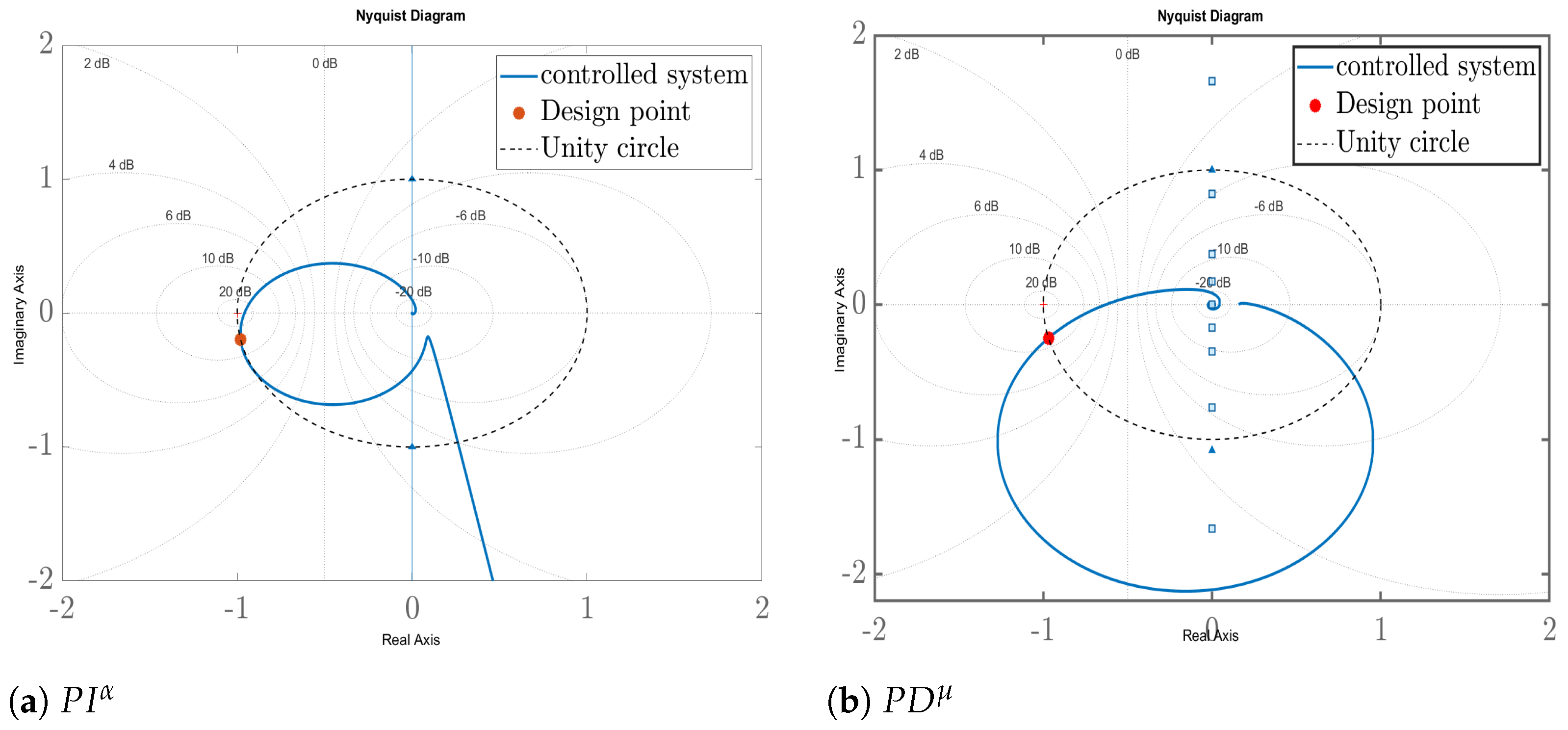
4. Fractional Order $\mathit{P}{\mathit{D}}^{\mathit{\mu }}$ Controller

In this section, we will examine the underdamped system represented by the transfer Function (1) and the fractional-order proportional-derivative controller

$$C_{PD}\left(s\right)=K_p+K_d·s^{\mu },0<\mu <2$$

(29)

$PD$ controllers are often used in mechatronics. In this sense, we have an interest in analyzing the fractional version of such a controller and calculating its feasible frequency specifications. In this sense, the condition of having a desired phase margin ${\varphi }_m$ and gaining a crossover frequency ${\omega }_c$ is expressed by

$$C_{PD}(j·{\omega }_c)·G(j·{\omega }_c)=-e^{j·{\varphi }_m}$$

(30)

From Equation (30), the normalized parameters of the $P{D}^{\mu }$ controller are expressed as a function of the normalized specifications ${\varphi }_{mn}$ and ${\omega }_{cn}$ by:

$$K_{dn}=\frac{Z_i}{{\omega }_{cn}^{\mu }·sin\left(\frac{\mu ·\pi }{2}\right)}$$

(31)

$$K_{pn}=Z_r-K_d·{\omega }_{cn}^{\mu }·cos\left(\frac{\mu ·\pi }{2}\right)$$

(32)

where:

$$Z_i=\Im \left(-e^{j·{\varphi }_{mn}}/G_n(j·{\omega }_{cn}))\right)$$

(33)

$$Z_r=\Re \left(-e^{j·{\varphi }_{mn}}/G_n(j·{\omega }_{cn}))\right)$$

(34)

In the case of the $P{D}^{\mu }$ control of a fractional-order process of the form (13), the resulting open-loop system does not have a pole at the origin. As a result, there is no stability constraint to adhere to the low-frequency behavior.

The phase margin is determined at the highest frequency where the magnitude of the open-loop system $C_{P{D}_n}(j·\omega )·G_n^{*}(j·\omega )$ is equal to unity. Here, $C_{P{D}_n}(j·\omega )$ represents the frequency response of the normalized $P{D}^{\mu }$ controller.

4.1. Robust High-Frequency Condition

The robust high-frequency condition stipulates that the magnitude of the frequency response should strictly decrease within the unit circle. This condition can be expressed as:

$${\left.\frac{d\left|C_{P{D}_n}(j·\omega )·G_n^{*}(j·\omega )\right|}{d\omega }\right|}_{\omega >{\omega }_{cn}}<0$$

(35)

It is a challenging task to find analytical formulae that guarantee the fulfillment of this condition for the normalized process (13) combined with the normalized $P{D}^{\mu }$ controller across all combinations of fractional-order operators $\mu$ and $\lambda$. Therefore, Figure 10 illustrates the three-dimensional region that defines the $RHFC$ in terms of the normalized specifications ${\omega }_{cn}$ and ${\varphi }_{mn}$ and the fractional order of the process $\lambda$. Moreover, these are the points that guarantee the $RHFC$ for any value $\mu \in (0,2]$.

Figure 10. $RHFC$ for $\lambda \in [1,2]$.

Since the $P{D}^{\mu }$ controller does not have a low-frequency condition, the red surfaces in Figure 10 correspond to the $RHFC$. Unlike the $P{I}^{\alpha }$ controller, this figure displays broad zones, even for process orders close to 2.

4.2. Modified $P{D}^{\mu }$ Controller

When analyzing the feasible frequency conditions obtained for each of the two controllers $P{I}^{\alpha }$ and $P{D}^{\mu }$ for the case of a delayed fractional order system with an underdamped step response, it is evident that:

For the case of $P{I}^{\alpha }$:

• It eliminates the steady-state error with the integral action.
• It presents two drawbacks: (a) very reduced regions for $\lambda$ close to 2, which clearly limits the design operation, (b) the relative stability is reduced.

For the case of $P{D}^{\mu }$:

• The regions of feasible frequency specifications are very extended compared to the case of a $P{I}^{\alpha }$.
• It increases relative stability.
• The main drawbacks are: (a) it increases the sensitivity to noise and (b) it cannot eliminate the steady-state error.

Therefore, in this section, we propose a new alternative that combines the advantages of both controllers. We modify the standard control scheme by incorporating feedback from the system’s output in such a way that we impose a fictitious pole at the origin of our fractional order model. This approach allows us to eliminate the static error. Subsequently, we design the $P{D}^{\mu }$ controller while ensuring that it meets the desired specifications.

Let us consider the positive feedback loop of Figure 11 applied to the process (1). Its closed-loop transfer function is

$$F_{cl}\left(s\right)=\frac{G\left(s\right)}{1-\delta ·G\left(s\right)}=\frac{K·e^{-\tau ·s}}{1+T·s^{\lambda }-\delta ·K·e^{-\tau ·s}}$$

(36)

Figure 11. Modified dynamic system.

If we impose $\delta =\frac{1}{K}$ in the previous equation we obtain:

$$F_{cl}\left(s\right)=\frac{K·e^{-\tau ·s}}{T·s^{\lambda }+(1-e^{-\tau ·s})}$$

(37)

In addition, using the Taylor series expansion, the term $(1-e^{-\tau s})$ can be approximated as $\tau s-\frac{{\tau }^2}{2}{s}^2+\dots$ Therefore, considering that $\lambda >1$, the resulting model features a pole at the origin of order 1 which enables us to eliminate the static error.

The resulting closed-loop scheme is shown in Figure 12, in which disturbances $z_1$ and $z_2$ have been included at the input of the process and the output measurement, respectively. The closed-loop transfer function assuming no disturbances, is:

$$Y\left(s\right)=\frac{K·e^{-\tau ·s}·C\left(s\right)}{1-K·\delta ·e^{-\tau ·s}+K·e^{-\tau ·s}·C\left(s\right)+T·s^{\lambda }}·Y^{*}\left(s\right)$$

(38)

Figure 12. Closed-loop control scheme considering the modified dynamic system.

If $K·\delta =1$, Expression (38) becomes

$$Y\left(s\right)=\frac{K·e^{-\tau ·s}·C\left(s\right)}{1-e^{-\tau ·s}+K·e^{-\tau ·s}·C\left(s\right)+T·s^{\lambda }}·Y^{*}\left(s\right)$$

(39)

It is easy to verify, by applying the Final Value Theorem, that the response of this system to a step command $Y^{*}\left(s\right)$ has zero steady-state error.

Let us study the characteristic equation of the transfer Function (39). It is expressed by

$$\begin{array}{c}1-e^{-\tau ·s}+K{e}^{-\tau ·s}C\left(s\right)+T·s^{\lambda }=0\Rightarrow (1+T·s^{\lambda })+K{e}^{-\tau ·s}\left(C\left(s\right)-\frac{1}{K}\right)=0\\ \Rightarrow 1+\frac{K{e}^{-\tau ·s}}{1+T·s^{\lambda }}(C\left(s\right)-\delta )=0\end{array}$$

(40)

If we denote $\widehat{C}\left(s\right)=C\left(s\right)-\delta$, this equation becomes $1+G\left(s\right)·\widehat{C}\left(s\right)=0$. Then the closed-loop specifications of this modified control system can be achieved using the $RHFC$ region of Figure 10 to design controller $\widehat{C}\left(s\right)=K_p+K_d·s^{\mu }$. After, the $P{D}^{\mu }$ controller $C\left(s\right)$ of Figure 12 is obtained from

$$C\left(s\right)=\widehat{C}\left(s\right)+\delta =K_p+\delta +K_d·s^{\mu }$$

(41)

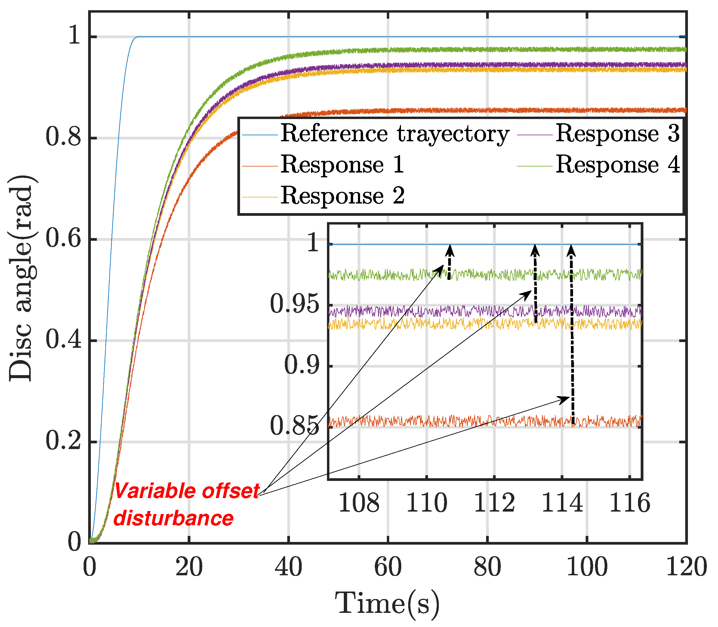
4.3. Disturbance Rejection Analysis

Consider Figure 12 and step disturbances in $z_1\left(t\right)$ and $z_2\left(t\right)$.

4.3.1. Case 1: Variable Step Disturbance at the Input of the Process

In this case $Z_1\left(s\right)=\frac{a}{s}$, where a is the amplitude of the step, and $Z_2\left(s\right)=0$. Simplifying the scheme of Figure 12, $Y\left(s\right)$ is expressed as a function of the reference $Y^{*}\left(s\right)$ and the disturbance $Z_1\left(s\right)$:

$$Y\left(s\right)=\frac{K·e^{-\tau ·s}·Z_1\left(s\right)+K·e^{-\tau ·s}·C\left(s\right)·Y^{*}\left(s\right)}{1-K·\delta ·e^{-\tau ·s}+K·e^{-\tau ·s}·C\left(s\right)+T·s^{\lambda }}$$

(42)

If $K·\delta =1$ then

$$Y\left(s\right)=\frac{K·e^{-\tau ·s}·Z_1\left(s\right)+K·e^{-\tau ·s}·C\left(s\right)·Y^{*}\left(s\right)}{1-e^{-\tau ·s}+K·e^{-\tau ·s}·C\left(s\right)+T·s^{\lambda }}$$

(43)

which has zero steady-state error to a step command $Y^{*}\left(s\right)$ and a steady state output $y_d=a/C\left(0\right)=a/(K_p+\delta )$ to the step disturbance $Z_1\left(s\right)$. Then the $P{D}^{\mu }$ cannot completely remove the steady-state error caused by disturbance $Z_1\left(s\right)$.

4.3.2. Case 2: Variable Step Disturbance at the Measurement of the Output of the Process

In this case $Z_1\left(s\right)=0$ and $Z_2\left(s\right)=\frac{a}{s}$ where a is the amplitude of the step. Simplifying the scheme of Figure 12, $Y\left(s\right)$ is expressed as a function of the reference $Y^{*}\left(s\right)$ and the disturbance $Z_2\left(s\right)$:

$$Y\left(s\right)=\frac{-K·e^{-\tau ·s}·\left(C\left(s\right)-\delta \right)·Z_2\left(s\right)+K·e^{-\tau ·s}·C\left(s\right)·Y^{*}\left(s\right)}{1-K·\delta ·e^{-\tau ·s}+K·e^{-\tau ·s}·C\left(s\right)+T·s^{\lambda }}$$

(44)

If $K·\delta =1$ then

$$Y\left(s\right)=\frac{-K·e^{-\tau ·s}·\left(K_p+K_d·s^{\mu }\right)·Z_2\left(s\right)+K·e^{-\tau ·s}·C\left(s\right)·Y^{*}\left(s\right)}{1-e^{-\tau ·s}+K·e^{-\tau ·s}·C\left(s\right)+T·s^{\lambda }}$$

(45)

which has zero steady-state error to a step command $Y^{*}\left(s\right)$ and a steady state output $y_d=-a·\left(C\left(0\right)-\delta \right)/C\left(0\right)=-a·K_p/(K_p+\delta )$ to the step disturbance $Z_2\left(s\right)$. Then the $P{D}^{\mu }$ can completely remove the steady state error caused by disturbance $Z_2\left(s\right)$ if $K_p=0$, i.e., if $C\left(s\right)=\delta +K_d·s^{\mu }$.

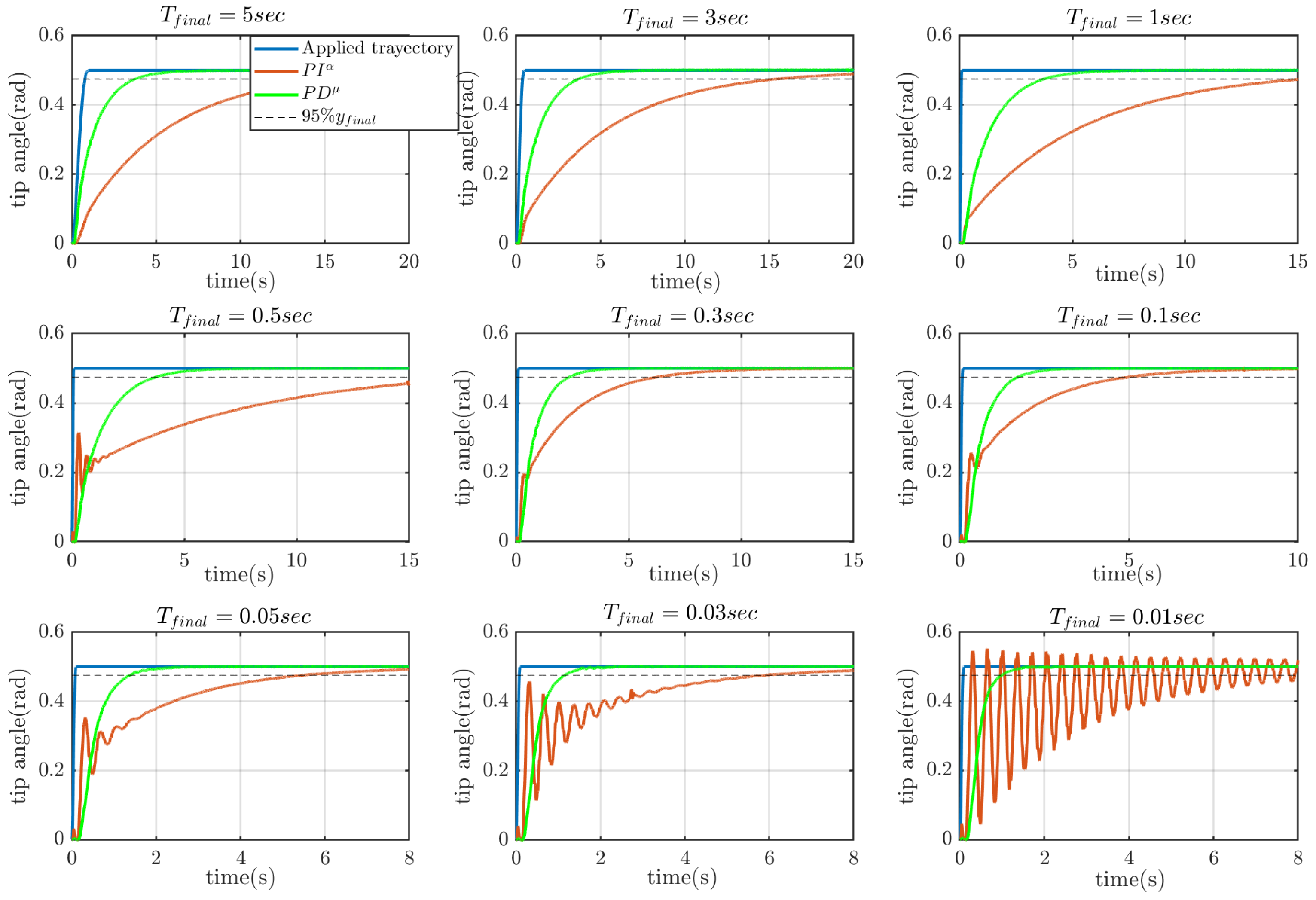
5. Application to the Control of Flexible Manipulator

5.1. Presentation of the Platform

Figure 13 provides a detailed depiction of the experimental platform, including all its components. The platform comprises a three-legged metallic structure that supports a Harmonic Drive mini servo $DC$ motor, specifically the model $RH-8D-6006-E036AL-SP\left(N\right)$. This motor features a reduction ratio of $n=25$.

Figure 13. Experimental platform: flexible manipulator robot.

This frame enables stable and unrestricted rotation of the motor in the horizontal plane around the vertical axis of the platform. The motor is characterized by the following parameter values: inertia $J=6.87\times {10}^{-5}$ $\mathrm{kg}·{\mathrm{m}}^2$, viscous friction $\nu =1.041\times {10}^{-3}$ $\mathrm{N}·\mathrm{m}·\mathrm{s}$, and electromechanical constant $k=0.21$ $\mathrm{N}·\mathrm{m}/\mathrm{V}$.

The servo-amplifier is designed to accept control inputs from the computer within the range of $[-10,10]$ volts. The flexible link is connected to the motor, and a load (disc) is positioned above the surface of an air table in a manner that nullifies the effects of friction and gravity. The disc is attached at its center to the end of the beam with a freely pivoted pin joint. The flexible link possesses the following characteristics: length $L_b=0.5$ m, cross-sectional diameter $d=3\times {10}^{-3}$ m, and flexural rigidity $EI=0.260$ N·m${}^2$.

The nominal tip load is a wood disc of mass $m_0=0.09$ kg. Because the mass of the link is small compared to that of the disc and because the pinned joint prevents the generation of torques at the end of the beam, this mechanical system has a single vibration mode. Then the nominal vibration angular velocity of the link is characterized as ${\omega }_0=5.8434$ rad/s ($f_0=0.93$ Hz).

The sensor system consists of an encoder embedded in the motor—which allows us to know the motor angular position ${\theta }_m\left(t\right)$ with a precision of $7·{10}^{-5}$ rad—and a pair of strain gauges with gauge factor $2.16$ and resistance $120.2\Omega$ that give the moment at the base of the link $\Gamma \left(t\right)$, i.e., the coupling torque between the motor and the link. The sampling time in the signals processing is $T_s=2$ ms.

5.2. The Dynamic Model

The dynamics of the described system, composed by the attachment of the flexible beam and the payload disc, was studied and experimentally identified in [36] yielding an underdamped fractional model of order $\lambda =1.92$:

$$G_b\left(s\right)=\frac{{\theta }_d\left(s\right)}{{\theta }_m\left(s\right)}=\frac{{\omega }_0^2}{s^{\lambda }+{\omega }_0^2}$$

(46)

and

$$G_{\Gamma }\left(s\right)=\frac{\Gamma \left(s\right)}{{\theta }_m\left(s\right)}=\frac{c·s^{\lambda }}{s^{\lambda }+{\omega }_0^2}{e}^{-\tau ·s}$$

(47)

where ${\theta }_d$ is the robot tip (disc) angle and c is an identified coefficient that characterizes the stiffness of the beam and the calibration of the strain gauge sensor.

5.3. Control Design and Analysis of the Results

The disc angle ${\theta }_d\left(t\right)$ can be estimated from the measurements using expression [37]:

$${\theta }_d\left(t\right)={\theta }_m\left(t\right)-\frac{\Gamma \left(t\right)}{c}$$

(48)

Then, a two-nested control loop scheme can be implemented. The inner loop controls the motor angular position feeding back ${\theta }_m$ measurements, and the outer loop controls the tip angular position by feeding back ${\theta }_d$ estimated by (48).

In the inner loop, the motor angle ${\theta }_m$ is corrected using a robust 2 $DOF$ $PID$ controller designed based on a pole placement technique and including compensation terms of the Coulomb friction and the motor-beam coupling torque. Besides removing disturbance effects, this inner loop is designed to be as fast as possible without saturating the actuator. Then a feedback loop with high-gain controllers is implemented. Details of this servo motor system can be found in [38]. The equivalent transfer function of the inner loop is

$$M\left(s\right)=\frac{{\theta }_m\left(s\right)}{{\theta }_m^{*}\left(s\right)}=\frac{1}{{\left(1+ϵ·s\right)}^2}$$

(49)

where ${\theta }_m^{*}$ is the reference to be followed by the output ${\theta }_m$ of the inner loop and $ϵ$ is made as small as possible.

The inner loop is implemented “in situ” while the outer control loop is assumed to be implemented in a remote station. Then the time delay is implemented between the output of the outer loop controller $u\left(t\right)$ and the input of the inner loop control system ${\theta }_m^{*}$. Consequently, the complete dynamic model of the robot, including the inner loop dynamics and the time delay, is

$$G\left(s\right)=\frac{{\theta }_d\left(s\right)}{u\left(s\right)}=\frac{{\omega }_0^2}{s^{\lambda }+{\omega }_0^2}·M\left(s\right)·e^{-\tau ·s}$$

(50)

We have artificially implemented a time delay in the output of the outer loop controller in order to simulate a teleoperated robotic system. Previous works on the teleoperation of flexible manipulators report time delays between one-tenth and the value of the period of the main vibration mode (the one with the lowest frequency of vibration) [39]. This period in the case of the nominal disc is $1.0753$ s. We have therefore implemented a time delay of $\tau =0.1613$ s, which is $15\%$ of the period of the main vibration mode of the flexible link.

Moreover, the inner loop has been designed such that $ϵ=0.0125$, i.e., the double pole of $M\left(s\right)$, is located at $-80$. Then the absolute value of this pole is more than ten times bigger than the vibration angular velocity of the beam, allowing us to assume that the inner loop dynamics are much faster than the dynamics involved in the outer loop. We can therefore assume that $M\left(s\right)\approx 1$ and that

$$G\left(s\right)\approx \frac{{\omega }_0^2}{s^{\lambda }+{\omega }_0^2}·e^{-\tau ·s}=\frac{1}{1+\frac{1}{{\omega }_0^2}·s^{\lambda }}·e^{-\tau ·s}$$

(51)

where the right member of the equation expresses $G\left(s\right)$ in the standarized form (1).

Figure 14a shows the detailed control scheme using a $P{I}^{\alpha }$ controller in the outer loop. It can be observed the place where the artificial time delay has been implemented: the reference signal of the inner loop is the delayed output of the fractional-order controller used in the outer loop. Furthermore, a disturbance step signal d is incorporated, representing the offset of the strain gauge sensor. Figure 14b shows a simplified control scheme that is expressed in terms of the equivalent transfer functions of the subsystems involved in Figure 14a. Note that $\widehat{d}=d/c$ is introduced in Figure 14b.

Figure 14. $P{I}^{\alpha }$ based control scheme. ((a): General control scheme with the inner loop of the motor. (b): Simplified control scheme).

Figure 15 depicts the control scheme using a $P{D}^{\mu }$ controller in the outer loop. It is also a simplified scheme version expressed in terms of the equivalent transfer functions of the involved subsystems. In this figure, we have implemented the modified dynamic system by providing feedback on the disc angular position with a positive sign which, based on the analysis conducted in the preceding section, incorporates a fictitious pole at the origin. In our case, taking into account the right-hand side of Expression (51), we obtain that $\delta =1$.

Figure 15. $P{D}^{\mu }$ based control scheme.

For our teleoperated robot, we have conducted a design study for the $P{I}^{\alpha }$ and $P{D}^{\mu }$ controllers using the tuning method described in the previous sections. Figure 16 displays the $RHFC$ regions of both controllers, as well as the low-frequency condition, considering $\alpha =\mu =0.88$ (arbitrarily chosen). For the case of the $P{I}^{\alpha }$ controller (Figure 16a), the red region represents the overlap between the $RHFC$ condition and the low-frequency condition. Regarding the $P{D}^{\mu }$ controller (Figure 16b), as previously mentioned, there is no low-frequency condition as the controller does not have a pole at the origin. However, there is a secondary stability constraint referred to as the ’Stability condition’, which requires positive values for the proportional parameter $K_p+\delta$ of the controller represented here by the blue region. The intersection of this last with the $RHFC$ is presented in red color and presents then the feasible frequency region of the $P{D}^{\mu }$ controller.

Figure 16. RHFC region.

To carry out a fair comparison between the $P{I}^{\alpha }$ controller and the $P{D}^{\mu }$ controller, including the positive feedback proposed in this paper, we have imposed identical specifications for both controllers: a gain crossover frequency ${\omega }_c=6.86$ rad/s and a phase margin ${\varphi }_m=0.25$ rad.

The numerical expressions of the designed controllers are:

$$C_{P{I}^{\alpha }}=0.1219+\frac{0.1255}{s^{0.88}}$$

(52)

$$C_{P{D}^{\mu }}=0.0293+0.0256·s^{0.88}$$

(53)

Note that these are the real controllers $C\left(s\right)$ and not the normalized ones $C_n(s*)$ (see (14)). In the case of $P{D}^{\mu }$ controller, the proportional parameter $K_p$ of the normalized controller should be 1, according to Section 4.3.2, in order to eliminate the steady state error caused by the strain gauges offset. This gain becomes $(1/{\omega }_0^2)$ in the real controller, which is the value expressed in (53).

Figure 17 illustrates the Nyquist plots for both controllers. It is evident that both controllers fulfill the desired specifications. Furthermore, it is notable that the $P{D}^{\mu }$ controller provides an extra margin of robustness for the system compared to the $P{I}^{\alpha }$ controller: the minimum distance of the Nyquist plot to the point $\left(-1,0\right)$ is bigger using the $P{D}^{\mu }$ than using the $P{I}^{\alpha }$.

Figure 17. Nyquist-plots.

The flexible manipulator is controlled using a LABVIEW graphical interface. We have devised a second-order, smoothly differentiable trajectory with an amplitude of 0.5 radians to avoid motor saturation. The duration of the trajectory, denoted as $L_t$, is adjustable. The fractional-order operators $s^{-\alpha }$ and $s^{\lambda }$ have been implemented using the Grunwald-Letnikov approximation and the principle of short memory [40].

As mentioned in the platform description, a pair of strain gauges was utilized to measure the deformation of a flexible link and determine the coupling torque at the base of the robot. However, it is worth noting that strain gauge sensors can sometimes display a noticeable offset. This offset refers to an output reading that deviates from zero even in the absence of applied strain.

In the specific case of the employed sensory system, despite implementing a calibration procedure, the offset signal persisted throughout the movement until the final position of the disc. This led to a step disturbance characterized by a variable value instead of a consistent offset signal. Figure 18 illustrates the controlled final position of the disc when a proportional controller with $K_p=1$ is used. The experiment is repeated multiple times to demonstrate the non-constancy of the offset value.

Figure 18. Experimental demonstration of the offset of the Strain gauge sensory system.

During the experimentation, we recorded the position ${\theta }_d$ of the disc for various values of $L_t$. In Figure 19, it can be observed that both controllers exhibit stable behavior when operating with slow trajectories. However, the response of the $P{I}^{\alpha }$ controller is considerably slower due to the integration process. Additionally, the last three sub-figures illustrate the system’s response when $L_t<0.05$, which can be regarded as a step command. It is evident that the $P{I}^{\alpha }$ controller leads to a critically stable behavior, whereas the $P{D}^{\mu }$ controller demonstrates a strictly stable response.

Figure 19. Experimental- results.

The responses of Figure 19 prove that it is possible to eliminate the offset disturbance of the strain gauges in flexible manipulators without resorting to controllers with an integral term, which could decrease the relative stability of the closed-loop system and its robustness to payload variations. Additionally, differentiating the strain gauge signal to remove the offset would introduce noise to the closed-loop control and compromise the compensation of steady-state tip position errors.

Observing Figure 16, it becomes evident that the feasible frequency specification region for the $P{D}^{\mu }$ controller is more extensive than that of the $P{I}^{\alpha }$ controller. The latter exhibits the advantage of eradicating steady-state errors, a significant issue inherent in the strain gauge sensors employed in the studied application. The newly formulated control scheme takes all these constraints into account by introducing a fictitious pole at the origin, effectively eliminating static errors (as shown in Figure 19). Consequently, the system’s response becomes more rapid, capitalizing on the broader feasible frequency region offered by the $P{D}^{\mu }$ controller.

Finally, we mention that the phase margin specification used in this comparative study is small. It is caused by the small $RHFC$ region that we obtain if we use a $P{I}^{\alpha }$ controller (see Figure 16a). Figure 16b shows that the $P{D}^{\mu }$ controller yields a bigger $RHFC$ region that would allow larger phase margins.

6. Conclusions

In this paper, feasible frequency specification regions have been computed for both $P{I}^{\alpha }$ and $P{D}^{\mu }$ fractional-order controllers. However, the study has two limitations. Firstly, the analysis has been conducted specifically for delayed underdamped systems with a range of $1<\lambda ⩽2$. This choice was motivated by the fact that previous research has primarily focused on controlling delayed fractional-order monotonic systems with $0<\lambda ⩽1$, while neglecting the case where $\lambda >1$.

The second limitation of our study is that we have focused solely on the gain crossover frequency and phase margin as design specifications. We could have considered alternative pairs of specifications, such as gain margin and phase margin, which are more suitable for robustness analyses. However, our primary objective in this study was to explore the enhancements achievable in the closed-loop response of a system by designing frequency specifications that simultaneously improve time response specifications and robustness properties. To achieve this, we employed frequency domain techniques, which are better suited for fractional-order controllers than time domain techniques, and we selected the above frequency specifications because they are closely related to time specifications, such as damping and speed of response, while also providing indications of robustness properties.

Regions of feasible pairs of specifications $\left({\varphi }_m,{\omega }_c\right)$ were determined for each of the considered controllers, taking into account all the combinations of fractional-order operators for the model and the controller. These regions were obtained to ensure that the Bode plot of the closed-loop system passes through the designated design point of the complex plane (the desired point of the unity circumference). Additionally, these regions guarantee robust stability of the closed-loop system by enforcing that the magnitude of the frequency response of the open-loop controlled system be a strictly decreasing function after the Nyquist plot has entered the unity circle. By using a design method based on these regions, we ensure that:

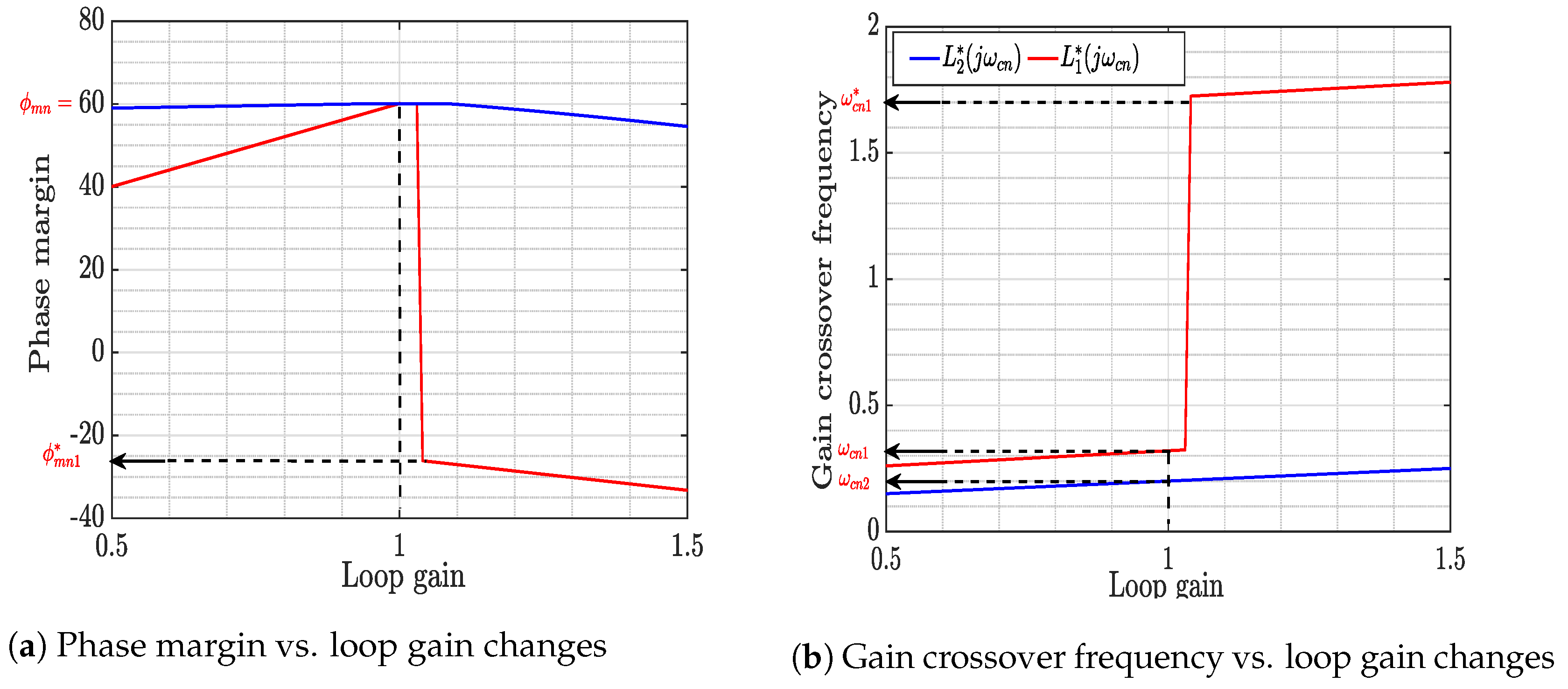
• The design specifications reflect the actual behavior of the closed-loop system, i.e., there are no frequencies beyond the gain crossover frequency at which the magnitude of the frequency response could be one, which could lead to different phase margin and gain crossover frequency specifications than the desired ones. In essence, the design method ensures that the selected specifications represent the true characteristics of the closed-loop system.
• Changes in the gain of the process (particularly increments of the gain) do not produce sharp changes in the phase margin and the gain crossover frequency that could suddenly unstabilize the closed-loop system. Note that this robustness concept is different from the well-known isophase margin condition. This one guarantees a local constant phase margin when the gain changes, while our condition guarantees that the phase margin changes smoothly in a broad range of gain variations. In particular, this smooth change is guaranteed if the gain grows with respect to the nominal value, which is the case that most likely can produce instability.

An application example involving the position control of a teleoperated flexible manipulator was developed in this study. Both $P{I}^{\alpha }$ and $P{D}^{\mu }$ controllers were designed to meet the same specifications for the system. The main challenge was to achieve the fastest and most precise response while eliminating the static error caused by the offset of the strain gauge sensor. To address this challenge, a modification was made to the system by implementing positive feedback on the angular position of the disc. This modification allowed for the introduction of a fictitious pole at the origin, which enabled the $P{D}^{\mu }$ controller to effectively eliminate the static error. As a result, the closed-loop system exhibited improved behavior and performance. Experimental results validated the controllers developed in this paper.

Our future research will address the obtention of Low-Frequency Conditions and Robust High-Frequency Conditions for $P{I}^{\alpha }{D}^{\mu }$ controllers.

References

- Abdulwasaa, M.A.; Abdo, M.S.; Shah, K.; Nofal, T.A.; Panchal, S.K.; Kawale, S.V.; Abdel-Aty, A.H. Fractal-fractional mathematical modeling and forecasting of new cases and deaths of COVID-19 epidemic outbreaks in India. Results Phys. 2021, 20, 103702. [Google Scholar] [CrossRef]
- AlBaidani, M.M.; Ganie, A.H.; Aljuaydi, F.; Khan, A. Application of Analytical Techniques for Solving Fractional Physical Models Arising in Applied Sciences. Fractal Fract. 2023, 7, 584. [Google Scholar] [CrossRef]
- Ahmad, I.; Ahmad, H.; Thounthong, P.; Chu, Y.M.; Cesarano, C. Solution of multi-term time-fractional PDE models arising in mathematical biology and physics by local meshless method. Symmetry 2020, 12, 1195. [Google Scholar] [CrossRef]
- Chen, W.; Sun, H.; Li, X. Fractional Derivative Modeling in Mechanics and Engineering; Springer: Berlin/Heidelberg, Germany, 2022. [Google Scholar]
- Srivastava, H.; Dubey, V.; Kumar, R.; Singh, J.; Kumar, D.; Baleanu, D. An efficient computational approach for a fractional-order biological population model with carrying capacity. Chaos Solitons Fractals 2020, 138, 109880. [Google Scholar] [CrossRef]
- Chen, S.B.; Jahanshahi, H.; Abba, O.A.; Solís-Pérez, J.; Bekiros, S.; Gómez-Aguilar, J.; Yousefpour, A.; Chu, Y.M. The effect of market confidence on a financial system from the perspective of fractional calculus: Numerical investigation and circuit realization. Chaos Solitons Fractals 2020, 140, 110223. [Google Scholar] [CrossRef]
- Shen, K.; Yu, W. Fractional programming for communication systems—Part I: Power control and beamforming. IEEE Trans. Signal Process. 2018, 66, 2616–2630. [Google Scholar] [CrossRef]
- Hekimoğlu, B. Optimal tuning of fractional order PID controller for DC motor speed control via chaotic atom search optimization algorithm. IEEE Access 2019, 7, 38100–38114. [Google Scholar] [CrossRef]
- Peng, X.; Shang, Y.; Zheng, X. Lower bounds for the blow-up time to a nonlinear viscoelastic wave equation with strong damping. Appl. Math. Lett. 2018, 76, 66–73. [Google Scholar] [CrossRef]
- Lewandowski, R.; Wielentejczyk, P. Nonlinear vibration of viscoelastic beams described using fractional order derivatives. J. Sound Vib. 2017, 399, 228–243. [Google Scholar] [CrossRef]
- Ding, X.; Zhang, G.; Zhao, B.; Wang, Y. Unexpected viscoelastic deformation of tight sandstone: Insights and predictions from the fractional Maxwell model. Sci. Rep. 2017, 7, 11336. [Google Scholar] [CrossRef]
- Xu, H.; Jiang, X. Creep constitutive models for viscoelastic materials based on fractional derivatives. Comput. Math. Appl. 2017, 73, 1377–1384. [Google Scholar] [CrossRef]
- Eldred, L.B.; Baker, W.P.; Palazotto, A.N. Kelvin-Voigt versus fractional derivative model as constitutive relations for viscoelastic materials. AIAA J. 1995, 33, 547–550. [Google Scholar] [CrossRef]
- Ogata, K. Modern Control Engineering; Prentice Hall: Upper Saddle River, NJ, USA, 2010; Volume 5, p. 894. [Google Scholar]
- Sanchis, R.; Romero, J.A.; Balaguer, P. Tuning of PID controllers based on simplified single parameter optimisation. Int. J. Control 2010, 83, 1785–1798. [Google Scholar] [CrossRef]
- Hamamci, S.E.; Tan, N. Design of PI controllers for achieving time and frequency domain specifications simultaneously. ISA Trans. 2006, 45, 529–543. [Google Scholar] [CrossRef] [PubMed]
- Castillo-Garcia, F.; Feliu-Batlle, V.; Rivas-Perez, R. Frequency specifications regions of fractional-order PI controllers for first order plus time delay processes. J. Process Control 2013, 23, 598–612. [Google Scholar] [CrossRef]
- Ariyatanapol, R.; Xiong, Y.P.; Ouyang, H. Partial pole assignment with time delays for asymmetric systems. Acta Mech. 2018, 229, 2619–2629. [Google Scholar] [CrossRef]
- Sinou, J.J.; Chomette, B. Active vibration control and stability analysis of a time-delay system subjected to friction-induced vibration. J. Sound Vib. 2021, 500, 116013. [Google Scholar] [CrossRef]
- Olgac, N.; Sipahi, R. Dynamics and stability of variable-pitch milling. J. Vib. Control 2007, 13, 1031–1043. [Google Scholar] [CrossRef]
- Gu, K.; Niculescu, S.I. Survey on recent results in the stability and control of time-delay systems. J. Dyn. Syst. Meas. Control 2003, 125, 158–165. [Google Scholar] [CrossRef]
- Li, S.; Zhu, C.; Mao, Q.; Su, J.; Li, J. Active disturbance rejection vibration control for an all-clamped piezoelectric plate with delay. Control Eng. Pract. 2021, 108, 104719. [Google Scholar] [CrossRef]
- Birs, I.; Muresan, C.; Nascu, I.; Ionescu, C. A survey of recent advances in fractional order control for time delay systems. IEEE Access 2019, 7, 30951–30965. [Google Scholar] [CrossRef]
- Shi, T.; Shi, P.; Wang, S. Robust sampled-data model predictive control for networked systems with time-varying delay. Int. J. Robust Nonlinear Control 2019, 29, 1758–1768. [Google Scholar] [CrossRef]
- Wu, M.; Cheng, J.; Lu, C.; Chen, L.; Chen, X.; Cao, W.; Lai, X. Disturbance estimator and smith predictor-based active rejection of stick–slip vibrations in drill-string systems. Int. J. Syst. Sci. 2020, 51, 826–838. [Google Scholar] [CrossRef]
- Araujo, J.M.; Santos, T.L. Control of second-order asymmetric systems with time delay: Smith predictor approach. Mech. Syst. Signal Process. 2020, 137, 106355. [Google Scholar] [CrossRef]
- Natori, K.; Oboe, R.; Ohnishi, K. Stability analysis and practical design procedure of time delayed control systems with communication disturbance observer. IEEE Trans. Ind. Inform. 2008, 4, 185–197. [Google Scholar] [CrossRef]
- Natori, K.; Oboe, R.; Ohnishi, K. Robustness on model error of time delayed control systems with communication disturbance observer. IEEJ Trans. Ind. Appl. 2008, 128, 709–717. [Google Scholar] [CrossRef]
- Zhou, W.; Wang, Y.; Liang, Y. Sliding mode control for networked control systems: A brief survey. ISA Trans. 2022, 124, 249–259. [Google Scholar] [CrossRef] [PubMed]
- Nian, F.; Shen, S.; Zhang, C.; Lv, G. Robust Switching Control for Force-reflecting Telerobotic with Time-varying Communication Delays. In Proceedings of the 2020 Chinese Control and Decision Conference (CCDC), Hefei, China, 22–24 August 2020; pp. 1714–1719. [Google Scholar]
- Rogers, G. Power System Oscillations; Springer Science & Business Media: Berlin/Heidelberg, Germany, 2012. [Google Scholar]
- Muresan, C.I.; Dutta, A.; Dulf, E.H.; Pinar, Z.; Maxim, A.; Ionescu, C.M. Tuning algorithms for fractional order internal model controllers for time delay processes. Int. J. Control 2016, 89, 579–593. [Google Scholar] [CrossRef]
- Abbisso, S.; Caponetto, R.; Diamante, O.; Fortuna, L.; Porto, D. Non-Integer Order Integration by Using Neural Networks. In Proceedings of the IEEE International Symposium on Circuits and Systems (Cat. No. 01CH37196), Sydney, Australia, 6–9 May 2001; Volume 3, pp. 688–691. [Google Scholar]
- Caponetto, R.; Dongola, G.; Pappalardo, F.; Tomasello, V. Auto-tuning and fractional order controller implementation on hardware in the loop system. J. Optim. Theory Appl. 2013, 156, 141–152. [Google Scholar] [CrossRef]
- Monje, C.A.; Chen, Y.; Vinagre, B.M.; Xue, D.; Feliu-Batlle, V. Fractional-Order Systems and Controls: Fundamentals and Applications; Springer Science & Business Media: Berlin/Heidelberg, Germany, 2010. [Google Scholar]
- Benftima, S.; Gharab, S.; Feliu-Batlle, V. Fractional Modeling and Control of Lightweight 1 DOF Flexible Robots Robust to Sensor Disturbances and Payload Changes. Fractal Fract. 2023, 7, 504. [Google Scholar] [CrossRef]
- Mamani, G.; Becedas, J.; Feliu-Batlle, V. Sliding mode tracking control of a very lightweight single-link flexible robot robust to payload changes and motor friction. J. Vib. Control 2011, 18, 1141–1155. [Google Scholar] [CrossRef]
- Gharab, S.; Benftima, S.; Batlle, V.F. Fractional Control of a Lightweight Single Link Flexible Robot Robust to Strain Gauge Sensor Disturbances and Payload Changes. Actuators 2021, 10, 317. [Google Scholar] [CrossRef]
- Yaryan, M.; Naraghi, M.; Rezaei, S.; Zareinejad, M.; Ghafarirad, H. Bilateral Nonlinear Teleoperation for Flexible Link Surgical Robot with Vibration Control. In Proceedings of the 2012 19th Iranian Conference of Biomedical Engineering (ICBME), Tehran, Iran, 20–21 December 2012; pp. 101–106. [Google Scholar]
- Podlubny, I. Fractional differential equations. Math. Sci. Eng. 1999, 198, 7–35. [Google Scholar]
Disclaimer/Publisher’s Note: The statements, opinions and data contained in all publications are solely those of the individual author(s) and contributor(s) and not of MDPI and/or the editor(s). MDPI and/or the editor(s) disclaim responsibility for any injury to people or property resulting from any ideas, methods, instructions or products referred to in the content. |
© 2023 by the authors. Licensee MDPI, Basel, Switzerland. This article is an open access article distributed under the terms and conditions of the Creative Commons Attribution (CC BY) license (https://creativecommons.org/licenses/by/4.0/).