Article

Robust Adaptive Fuzzy Fractional Control for Nonlinear Chaotic Systems with Uncertainties

by
Masoud S. Bahraini
1,2,*,
Mohammad Javad Mahmoodabadi
2 and
Niels Lohse
1
1
Intelligent Automation Centre, Wolfson School of Mechanical, Electrical & Manufacturing Engineering, Loughborough University, Loughborough LE11 3TU, UK
2
Department of Mechanical Engineering, Sirjan University of Technology, Sirjan 7813733385, Iran
*
Author to whom correspondence should be addressed.
Fractal Fract. 2023, 7(6), 484; https://doi.org/10.3390/fractalfract7060484
Submission received: 2 May 2023 / Revised: 10 June 2023 / Accepted: 14 June 2023 / Published: 18 June 2023
(This article belongs to the Section Engineering)

Abstract

:
The control of nonlinear chaotic systems with uncertainties is a challenging problem that has attracted the attention of researchers in recent years. In this paper, we propose a robust adaptive fuzzy fractional control strategy for stabilizing nonlinear chaotic systems with uncertainties. The proposed strategy combined a fuzzy logic controller with fractional-order calculus to accurately model the system’s behavior and adapt to uncertainties in real-time. The proposed controller was based on a supervised sliding mode controller and an optimal robust adaptive fractional PID controller subjected to fuzzy rules. The stability of the closed-loop system was guaranteed using Lyapunov theory. To evaluate the performance of the proposed controller, we applied it to the Duffing–Holmes oscillator. Simulation results demonstrated that the proposed control method outperformed a recently introduced controller in the literature. The response of the system was significantly improved, highlighting the effectiveness and robustness of the proposed approach. The presented results provide strong evidence of the potential of the proposed strategy in a range of applications involving nonlinear chaotic systems with uncertainties.

1. Introduction

The control of nonlinear chaotic systems with uncertainties is a challenging problem that has attracted significant research attention due to its wide range of applications in areas such as robotics, finance, and telecommunications. Nonlinear chaotic systems exhibit complex behaviors, including sensitivity to initial conditions, long-term unpredictability, and irregular oscillations. These behaviors make it difficult to design a robust and effective control strategy that can ensure the stability and performance of the system. A literature review revealed the extensive employment of various control methods for the stabilization and synchronization of chaos in nonlinear dynamics such as fractional-order PID control [1], adaptive control [2], adaptive H control [3], fuzzy adaptive control [4], sliding mode control (SMC) [5], and adaptive back-stepping control [6]. In recent years, several control strategies have been proposed to address this challenge, including fuzzy logic controllers, fractional-order calculus, and SMCs.
The SMC methodology can be implemented as a robust supervisory controller to provide necessary and sufficient control inputs when required. It has been effectively applied to various research fields due to its fundamental properties, such as robustness and accuracy against model parametric uncertainties. For example, Zhang [7] proposed time-dependent switching rules for an uncertain switched system using robust integral SMC. This method was based on a recursive searching method for the common Lyapunov function and a robust integral-type sliding mode surface design. The proposed method was shown to be effective in simulations and improved the system’s robustness and anti-disturbance performance from the initial time. However, the effectiveness of the proposed method depended on the accuracy of the system model and parameter design. Furthermore, Pradhan and Das [8] investigated a robust H sliding mode scheme for the load frequency control of time-delay interconnected power systems (IPSs) with actuator saturation and wind power integration. The proposed controller incorporated an artificial delay and was shown to effectively reduce frequency deviation in the IPS. A robust adaptive dynamic sliding mode approach was proposed by Hu and Wang [9] to control an automobile engine’s electronic throttle system. This proposed control scheme combined the advantages of adaptive sliding mode control and conventional robust controllers, and exhibited high tracking precision and robustness. The chattering phenomenon of the conventional sliding mode was significantly alleviated, and the stability proof of the closed-loop control system was presented by combining the observer dynamics with the feedback control system. Moreover, Ye and Wang [10] recommended robust adaptive integral terminal SMC in combination with an extreme learning machine (ELM) approach for the tracking control of a steer-by-wire system with uncertain dynamics. The proposed control ensured finite-time error convergence and estimated lumped uncertainty, reducing control chattering and simplifying selection of the switching gain. The ELM used for the estimation of the lumped uncertainty was regarded as an essential component of the closed-loop control and did not require any training process; the output weights were adaptively adjusted in reference to Lyapunov theory to ensure the global stability of the closed-loop control. Additionally, Zhou et al. [11] proposed an adaptive robust control scheme based on SMC and subjected to a nonlinear disturbance observer that can effectively solve challenges arising from parametric uncertainties and unknown time-varying external disturbances. The proposed controller handled the challenges of model uncertainty and unknown time-varying external disturbances. Van and Do [12] improved a robust fault-tolerant controller for a class of second-order uncertain nonlinear systems. The authors combined a sliding surface, a continuous control law, and an adaptive law to approximate unknown system dynamics. The crucial parameters of the controller were optimally selected using the Bat algorithm. The proposed approach provided several advantages, such as strong robustness, fast convergence, low steady-state error, and chattering-free [12]. A novel optimal robust fuzzy adaptive integral SMC model was designed via a multi-objective grey wolf optimization algorithm to stabilize a nonlinear uncertain chaotic system; its performance was evaluated using the Duffing–Holmes oscillator as a case study [13]. The designed controller stabilized the system errors using integral sliding surfaces and a sliding mode stabilizer where the design gains of the integral SMC were adapted using the gradient descent approach, and fuzzy logic systems were used to regulate the coefficients of the proposed robust control approach. Finally, a hybrid robust adaptive SMC was proposed in [14] that combines different control strategies for partially known plants. The controller was shown to be globally stable and robust through Lyapunov stability analysis and numerical simulations. The proposed methodology is feasible for regulating partially modeled plants and can be extended to multiple steps ahead. However, the increase in the number of parameters to be identified may affect the assumptions of the model and the performance of the controller.
Recently, researchers have focused on the adaptive tuning of feedback control parameters. For instance, Chiang and Lin [15] investigated an adaptive fuzzy controller with self-tuning fuzzy sliding-mode compensation for hydraulic-pump-controlled servo systems. Kim [16] modeled a cascade output voltage control law based on the self-tuning adaptive inner and outer-loop controllers for a nonlinear converter. Tavakoli and Seifi [17] proposed an adaptive self-tuning proportional–integral–derivative fuzzy SMC model with a switching surface to suppress the oscillations of power systems. Roman et al. [18] optimally tuned the parameters of a dynamic linearization-PD Takagi–Sugeno fuzzy algorithm in a model-free manner via virtual reference feedback tuning. Furthermore, Scheinker et al. [19] presented an adaptive model tuning approach based on real-time accelerators to continuously predict the longitudinal phase space of electron beams. The adaptive tuning of feedback control parameters can bring several benefits to a control system, such as improved performance by adjusting the parameters in real time, increased robustness to disturbances and parameter uncertainties, and reduced tuning time compared with manual methods, leading to more accurate control. However, this approach also presents some challenges, such as increased complexity and computational resources, model dependency that can cause poor performance or instability if the model is inaccurate, implementation challenges that require specialized hardware and software, and the risk of oscillations if the tuning is inadequate.
Moreover, of great importance for researchers in control theories is studying and developing fuzzy-logic-based systems with continuous values between 0 and 1 for false and true variables. Due to its unique advantages, these systems have been extensively utilized in a broad range of subjects. To name but a few, Borges et al. [20] developed a prototype for feeding solids and controlled it through fuzzy systems. The use of a fuzzy controller provided better results than an On–Off control for different feeding profiles. Fuzzy controllers had advantages over conventional PI and PID controllers in their study, as fuzzy controllers could deal with non-linear control functions and were easier to implement [20]. To attain a hybrid intelligent converter, a genetic-fuzzy control method was applied to an active free-piston Stirling engine by Masoumi et al. [21]. A fuzzy PID control scheme was proposed by Jin et al. [22] to improve the accuracy of the transplanting manipulator in the displacement tracking of a picking-up system. The authors designed a fuzzy PID controller to adjust PID parameters online. The control effects of conventional PID control and fuzzy PID control were compared, and it was found that the fuzzy PID control improved the stability and dynamic performance of the system, with a faster response time and no vibration compared with traditional PID control. The fuzzy tracking control of a class of uncertain linear dynamical systems was investigated in a study by Abbasi and Jalali [23]. These authors proposed two fuzzy control laws for the fuzzy tracking control problem of uncertain linear dynamical systems expressed as fuzzy differential equations. The first control law was in the form of a fuzzy state feedback with fuzzy gains and an additional pre-compensator term, while the second control law incorporated a granular integral pre-compensator to achieve disturbance rejection. The effectiveness of the proposed approaches was demonstrated through examples of two tanks in a series system and a landing jet aircraft. However, their paper suggested that future work should consider a combination of robust techniques and fuzzy control [23]. The simultaneous control of the surge speed and heading angle of a sailboat was investigated by Deng et al. [24]. Event-triggered composite adaptive fuzzy laws were developed to solve this problem. In addition, Nejadkourki and Mahmoodabadi [25] developed a fuzzy adaptive state-feedback control scheme for a revolute–prismatic–revolute (RPR) robot manipulator. Fuzzy-logic-based control theories offer several advantages for nonlinear chaotic systems. One of the main pros is that fuzzy logic controllers can handle complex nonlinear dynamics, which are difficult to model mathematically. Additionally, fuzzy logic controllers can demonstrate robust performance in the presence of uncertainties and disturbances. They can also be designed and implemented with relatively simple and intuitive rules, making them easier to understand and tune compared with other control methods. However, one of the drawbacks of fuzzy-logic-based control is that it can be difficult to design an optimal rule base, especially for highly nonlinear systems. Moreover, fuzzy-logic-based controllers may have limited performance when dealing with systems that have high-dimensional state spaces or rapidly changing dynamics. Finally, the interpretability of the control laws may be limited, which can make it difficult to understand the underlying mechanisms of the controller.
On the other hand, fractional calculus, as an incipient field in mathematics, has been extensively used in many branches of physics and engineering sciences, such as control systems [26,27,28,29,30], dynamical systems [31], viscoelastic materials [32,33,34], signal and image processing [35], diffusion wave [36], biomedical applications [37], stochastic and chaotic systems [38], and heat systems [39]. However, most studies published in the last three decades have concentrated on the fractional PID controller [40,41,42]. In recent years, there has been growing interest in controlling uncertain fractional-order nonlinear systems. A fractional adaptive backstepping control method was proposed in [43], which had the advantage of addressing the complexity issue of the common backstepping method by using a fractional command filter and the Szász–Mirakyan operator as a universal approximator. In addition, this method incorporated an efficient robust control term to handle approximation errors and unknown disturbances. In [44], the researchers proposed a compound adaptive fuzzy backstepping control strategy to synchronize two uncertain fractional-order chaotic systems with external disturbances. The approach incorporated a fuzzy logic system, a disturbance observer, fractional-order command filters, and error compensation signals to overcome the “explosion of complexity” issue and achieve satisfactory synchronization. Overall, fractional-order controllers provide a more flexible and accurate control approach by considering the non-integer order derivatives of the error signal. The fractional-order PID controller can adjust the proportional, integral, and derivative gains, as well as the fractional orders, to achieve optimal control performance [26]. However, the implementation of fractional-order controllers requires more computational effort. The tuning of the fractional-order controller parameters is also a challenging task, as the selection of the fractional orders is based on trial-and-error methods, which can be time-consuming and lead to suboptimal control performance.
Robust adaptive control is a control strategy that aims to tackle the problem of uncertainty in a system. This becomes especially important in nonlinear chaotic systems where external disturbances, parameter variations, and unmodeled dynamics can lead to significant uncertainty. Fuzzy control is a specific type of control strategy that employs fuzzy logic to map input variables to output variables. Fractional PID controllers, which introduce two additional fractional exponential terms of integral and derivative, have emerged as a popular alternative to conventional PID controllers. They provide better performance in terms of rise time, settling time, overshoot, and steady-state error while retaining a similar simple structure [45]. Additionally, the fractional terms enhance the controller’s flexibility, making it more robust and suitable for use in various engineering fields. In this paper, we propose a new control strategy called the Robust Adaptive Fuzzy Fractional PID (RAFFPID) controller, which combines the strengths of fuzzy logic controllers, fractional-order calculus, and SMCs to stabilize nonlinear chaotic systems with uncertainties. The proposed control strategy consists of two stages: a robust control stage for controlling chaotic behavior, and an adaptive fuzzy control stage for adapting the system to uncertainties. The Duffing–Holmes oscillator is used to evaluate the performance of the proposed controller. The Duffing–Holmes oscillator is a non-linear oscillator that is commonly used as a mathematical model for a wide range of phenomena in physics, engineering, and biology. The Duffing–Holmes oscillator is described by a second-order differential equation that includes a cubic nonlinearity; its behavior can be chaotic under certain conditions. The oscillator is often used as a test system for studying nonlinear dynamics and chaos theory, and it has applications in fields such as mechanical engineering, electronic circuit design, and neuroscience. This study shows the potential of the proposed approach for a range of applications involving nonlinear chaotic systems with uncertainties. The proposed control approach was further investigated through numerical simulation results by comprehensive comparisons with the literature to demonstrate its performance, effectiveness, and robustness.
In summary, the advantages of the proposed RAFFPID controller over the existing methods include the integration of multiple control strategies, robustness to uncertainties, adaptive tuning, multi-objective optimization, and improved performance compared with existing methods. These advantages make the proposed approach a promising solution for stabilizing nonlinear chaotic systems with uncertainties in various applications. The contributions of this research can be summarized as follows:
  • Proposed the RAFFPID controller, a novel control strategy that combines fuzzy logic controllers, fractional-order calculus, and sliding mode control to effectively stabilize nonlinear chaotic systems with uncertainties while accurately modeling the system’s behavior and adapting in real time.
  • Conducted a multi-objective optimization process to tune the controller parameters and balance the state errors of the system and its control input.
  • Evaluated the performance of the proposed controller on the Duffing–Holmes oscillator, a benchmark system that includes external uncertainties, and demonstrated that the proposed method outperforms a recently introduced controller in the literature.
To this end, the rest of this paper is organized as follows. Section 2 presents the theory and formulation of the proposed work. Section 3 provides the simulation results and the application of the introduced controller on uncertain chaotic systems, including the Duffing–Holmes oscillator. Finally, Section 4 concludes the paper.

2. Theory and Formulations of the Proposed Study

In this study, a class of nonlinear systems is considered by the following equations:
x ˙ 1 ( t ) = x 2 ( t ) x ˙ 2 ( t ) = f ( χ , t ) + g ( χ , t ) + D ( t ) + u ( t )
where the state vector of the system is represented by χ = [ x 1 , x 2 ] T . The system dynamics and uncertainties are expressed by unknown bounded nonlinear functions f ( χ , t ) and g ( χ , t ) , respectively. D ( t ) stands for the external bounded disturbances, and u ( t ) is the control signal. The positive constant, α, is considered to limit external disturbances so that | D ( t ) | < α . In addition, two upper bounds f u ( χ , t ) and g u ( χ , t ) are assumed for system dynamics and uncertainties so that | f ( χ , t ) | f u ( χ , t ) and | g ( χ , t ) | g u ( χ , t ) . Notably, the superscript “u” stands for “upper bounds” in f u ( χ , t ) and g u ( χ , t ) .
Furthermore, the error, e, is defined as the difference between the desired input and the real output. The desired input vector of the system is denoted as Y d = [ y d , y ˙ d ] T in which Y d is subject to || Y d || = s u p t 0 || Y d ( t ) || . Moreover, the error vector of the system can be defined as E = Y d χ = [ e , e ˙ ] T . Let K = [ k 1 , k 2 ] T to be chosen such that the roots of s 2 + k 2 s + k 1 = 0 lie on the left-hand side of the complex plane. Then, the feedback linearization control law can be formulated as follows:
u ( t ) = f ( χ , t ) g ( χ , t ) D ( t ) + y ¨ d + K T E .
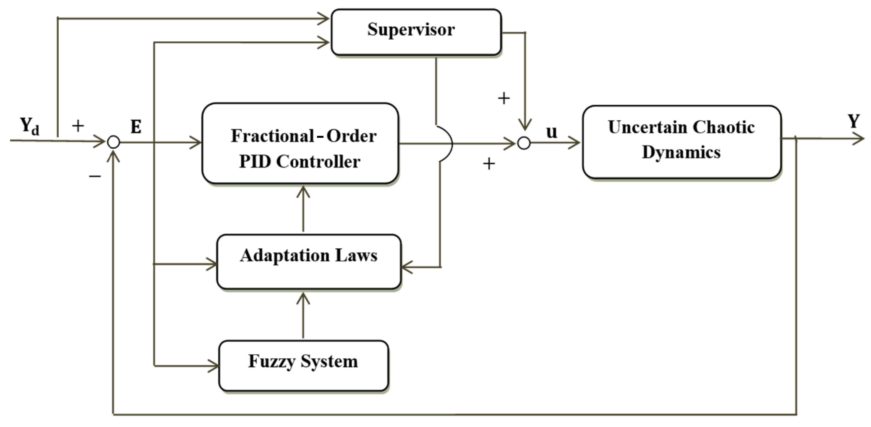
However, the control approach proposed in this paper combines a fractional-order PID controller with a supervised controller to enhance its performance. The resulting control signal for the considered second-order chaotic uncertain system is formulated as follows:
u ( t ) = u F O P I D ( t ) + u s ( t ) ,
where u F O P I D     is the fractional-order PID compensator, and u s stands for the supervisory control term. The structure of the proposed controller can be summarized as the four stages shown in Figure 1.

2.1. Fractional-Order PID Control

A fractional PID controller is an extension of the classical proportional integral derivative stabilizers based on fractional-order calculus. To implement this type of controller, five parameters need to be tuned, including the coefficient of proportional, integral, and derivative terms, in addition to the orders of the fractional integral and derivative terms. In a simple notation, the fractional PID controller can be represented by the following equation:
u F O P I D ( t ) = k p e ( t ) + k i D λ e ( t ) + k d D μ e ( t ) ,
where kp, ki, and kd are the proportional, integral, and derivative constant gains, respectively. Moreover, λ is the order of fractional integration, and μ is the order of fractional differentiation. The error signal, e(t), is the difference between the desired input, y d ( t ) , and its actual output, y ( t ) , which can be expressed as follows:
e ( t ) = y d ( t ) y ( t ) .

2.2. Adaptation Laws

To obtain the adaptation laws for tuning and updating three gains of the fractional PID controller (kp, ki, and kd), the time derivative of the regulation signal, q r , is defined as follows.
q ˙ r = y ¨ d + k 2 e ˙ + k 1 e .
Furthermore, the sliding surface, S , can be obtained via the following equation:
S = x 2 ( t ) q r ( t ) .
When the system settles at the sliding mode, ( S = 0 ) , then x 2 = q r and
x ˙ 2 = y ¨ d + k 2 e ˙ + k 1 e .
Hence, if k 1 and k 2 are appropriately assigned, the error tends to zero as time trends to infinity. To investigate the stability of the system, a proper Lyapunov function can be defined as follows:
V = S 2 2 .
To guarantee the stability of the system, the time derivative of the Lyapunov function must be negative definite:
V ˙ = S S ˙ < 0 .
Substituting the nonlinear Equation (1) into the time derivative of Equation (7) yields:
S ˙ = x ˙ 2 ( t ) q ˙ r ( t ) = f ( χ , t ) + g ( χ , t ) + D ( t ) + u ( t ) q ˙ r ( t ) .
By employing Equation (3) and multiplying S by both sides of Equation (11), we have:
S S ˙ = S ( f ( χ , t ) + g ( χ , t ) + D ( t ) + u F O P I D ( t ) + u s ( t ) q ˙ r ( t ) ) .
Consequently, the three fractional-order PID coefficients will be updated by employing the gradient descent approach and the chain differentiation rule as follows:
k ˙ p = γ S S ˙ k p = γ S S ˙ u F O P I D u F O P I D k p = γ 1 S e ( t ) ,
k ˙ i = γ S S ˙ k i = γ S S ˙ u F O P I D u F O P I D k i = γ 2 S D λ e ( t ) ,
k ˙ d = γ S S ˙ k d = γ S S ˙ u F O P I D u F O P I D k d = γ 3 S D μ e ( t ) ,
where γ 1 , γ 2 , and γ 3 denote learning rates.

2.3. Supervisory Controller

The supervisory controller should be designed such that the states of the system are held around predetermined limited regions. Substituting Equations (2) and (3) into Equation (1) yields:
x ˙ 2 ( t ) = y ¨ d + K T E ( u ( t ) u F O P I D ( t ) u s ( t ) ) .  
By applying the error signal e = y d x 1 , it can be obtained that:
e ¨ = K T E + ( u ( t ) u F O P I D ( t ) u s ( t ) ) ,
where E and K are chosen as E = [ e 1 e 2 ] T and K = [ k 1 k 2 ] T for the considered second-order nonlinear equation. By defining A and B as follows:
A = [ 0 1 k 1 k 2 ] ,
B = [ 0 1 ] T .
Equation (17) can be rewritten as:
E ˙ = A E + B ( u ( t ) u F O P I D ( t ) u s ( t ) ) .
The candidate Lyapunov function can be chosen as:
V e = 1 2 E T P E ,
where P as a positive definite symmetric matrix is obtained from the Lyapunov equation as follows:
A T P + P A = Q ,
and Q is a positive definite symmetric matrix where its components can be determined by the designer. We define:
V M = 1 2 λ m i n ( P ) ( M x || Y d || ) 2 ,
where M x is a pre-specified parameter, V M is a positive constant, and λ m i n ( P ) represents the minimum eigenvalue of P. Notably, if || χ || M x , then, from (21), we can write:
V e 1 2 λ m i n ( P ) || E || 2 1 2 λ m i n ( P ) ( || χ || || Y d || ) 2 1 2 λ m i n ( P ) ( M x || Y d || ) 2 = V M .
Hence, if V e < V M , then || χ || < M x . Moreover, by substituting Equations (20) and (21) into the time differentiation of Ve, the following relation is obtained:
V ˙ e = 1 2 E T ( A T P + P A ) E + E T P B ( u u F O P I D u s )         = 1 2 E T Q E + E T P B ( u u F O P I D u s )           1 2 E T Q E + | E T P B | ( | u | + | u F O P I D | ) E T P B   u s .
Considering bounded functions | f ( χ , t ) | f u ( χ , t ) , | g ( χ , t ) | g u ( χ , t ) and | D ( t ) | α in Equation (2) leads to the following relation:
u ( t ) f u ( χ , t ) + g u ( χ , t ) + α + | y ¨ d | + | K T E | .
Therefore, to satisfy V ˙ e 0 , the supervisory controller is proposed as follows:
u s ( t ) = { 0               i f || χ || M x                                                                                                                                         s g n ( E T P B ) ( f u ( χ , t ) + g u ( χ , t ) + α + | y ¨ d | + | K T E | + | u F O P I D ( t ) | ) i f || χ || M x  
If || χ || M x , then V ˙ e 0 and Equations (26) and (27) guarantee the stability of the system.
V ˙ e 1 2 E T Q E + | E T P B | ( | u | + | u F O P I D | ) E T P B   u s         = 1 2 E T Q E + | E T P B | ( | u | + | u F O P I D | s g n ( E T P B ) ( f u + g u + α + | y ¨ d | + | K T E | | u F O P I D | ) )           1 2 E T Q E 0 .
It should be noted that the update laws for the proposed controller are designed to satisfy the Lyapunov function by ensuring that the derivative of the Lyapunov function is negative semi-definite. As shown in Equation (28), the derivative of the Lyapunov function depends on the update laws and the input signals, which are bounded according to the assumptions made in Equation (2). By selecting appropriate design parameters, such as the gain matrix K and the parameters in the update laws, the stability of the closed-loop system can be guaranteed. Therefore, the update laws are crucial for the stability analysis, designed in a way that satisfies (10).

2.4. Fuzzification of the Learning Rates

Fuzzy-logic-based systems have gained widespread use in various real-world applications due to their ability to transfer expert knowledge into practical systems. However, the construction of the fuzzy rule base and rule regulation can be a time-consuming and iterative process. In this study, we propose a method to tune the numerical values of learning rates γ 1 , γ 2 , and γ 3 . Specifically, we utilize the fuzzifier, inference engine, and defuzzifier components with singleton, product, and center average formulations, respectively, in Equation (29):
γ i f = j = 1 N     μ A j ( e   ) y ¯ j j = 1 N     μ A j ( e   ) ,   i = 1 , 2 , 3
where y ¯ j is the center of the output membership functions defined in Table 1, and N = 3 is the number of rules. In addition, input membership functions, μ A j ( e   ) , are defined as follows:
μ A 1 ( e   ) = { 1                                                                             e < 1 e                                                       1 e 0       0                                                                                   e > 0
μ A 2 ( e   ) = { 0                                                                                       e < 1 e + 1                                                     1   e 0     e + 1                                                               0 < e < 1 0                                                                                               e > 1
μ A 3 ( e   ) = { 0                                                                             e < 0 e                                                               0 e 1     1                                                                                   e > 1
The schematic representation of these memberships is illustrated in Figure 2. Finally, the learning rates can be computed by employing the following equation:
γ i = γ i c + γ i p γ i f ,     i = 1 , 2 , 3
in which γ i c and γ i p , as the constant parameters, would be found through the multi-objective optimization process. This approach streamlines the process of constructing fuzzy-logic-based systems and enables the automatic tuning of key parameters, leading to more efficient and accurate systems.
In summary, to fuzzify the learning rates, input membership functions μ A j ( e   ) are defined for each of the three learning rates: γ 1 , γ 2 , and γ 3 . The input data, e, are regarded as these membership functions using Equations (30)–(32). Then, we use the fuzzifier, inference engine, and defuzzifier components to obtain the fuzzy values of the learning rates. Specifically, we employ the singleton, product, and center average formulations to perform fuzzification, inference, and defuzzification, respectively. These produce three fuzzy values, γ 1 f , γ 2 f , and γ 3 f , then constant parameters, γ 1 c , γ 2 c , and γ 3 c , and proportional parameters, γ 1 p , γ 2 p , and γ 3 p , are added to them to obtain the final values of learning rates, γ 1 , γ 2 , and γ 3 .

3. Simulation and Discussions

3.1. Duffing–Holmes Chaotic Oscillator—Example 1

The Duffing–Holmes chaotic system is chosen to challenge the performance of the proposed RAFFPID control scheme. The dynamical equations of the considered Duffing–Holmes system are represented as follows [46]:
{ x ˙ 1 ( t ) = x 2 ( t ) x ˙ 2 ( t ) = x 1 ( t ) 1 4 x 2 ( t ) x 1 3 ( t ) + 3 10 cos ( t ) + g ( χ , t ) + D ( t ) + u ( t )
where the uncertainty function g ( χ , t ) and external disturbance D ( t ) are defined as follows:
g ( χ , t ) = 0.1 s i n ( t ) ( x 1 ( t ) ) 2 + ( x 2 ( t ) ) 2
D ( t ) = 0.1 s i n ( t )
Hence, the related upper bounds can be defined as follows:
f u = | x 1 ( t ) | + 0.25 | x 2 ( t ) | + | x 1 3 ( t ) | + 0.3
g u = 0.1 x 1 2 ( t ) + x 2 2 ( t )
To implement the multi-objective optimization operation on the Duffing–Holmes system, objective functions M1 and M2 can be defined by:
M 1 ( μ ) = 0 τ ( | e 1 ( t ) | + | e 2 ( t ) | ) d t ,
M 2 ( μ ) = 0 τ | u ( t ) | d t + m a x t = 0 τ | u ( t ) | ,
where e 1 ( t ) = y d ( t ) x 1 ( t ) and e 2 ( t ) = y ˙ d ( t ) x 2 ( t ) are the differences between the desired values and actual values, respectively. Furthermore, m a x t = 0 τ | u ( t ) | indicates the maximum absolute value of the control signals from time 0 to τ. The final time, τ, is chosen as 30 (s) during the simulation process to ensure that the states of the system are converged to the desired trajectories.
To validate the accuracy of the proposed controller, the performance of the introduced RAFFPID scheme is compared with that of robust adaptive PID control subject to sliding modes and fuzzy rules (RAPIDC-S&F) presented in [46]. Herein, a multi-objective optimization approach based on the genetic algorithm is used to find the optimum gains of the RAFFPID and RAPIDC-S&F controllers. Two sets of the initial conditions are chosen as Set 1: x 1 (0) = 0.2 and x 2 (0) = 0.2, and Set 2: x 1 (0) = 0.5 and x 2 (0) = −0.7. Representative sets of the Pareto optimal solutions are plotted in Figure 2 and Figure 3 for the objective functions defined in Equations (39) and (40) and found by using the two controllers. It is noticeable that the implementation time is 30 s for the results illustrated in Figure 3 and Figure 4. As shown in these figures, a significant improvement in the values of the objective functions is represented by applying the proposed controller. From Figure 3, it can be seen that the minimum values of the objectives are M 1 = 1.015 and M 2 = 42.14 for the RAPIDC-S&F [46], while those are M 1 = 0.38 and M 2 = 19.19 for the proposed controller. The significant changes in the objective values can also be observed in Figure 4 for the initial conditions of Set 2, where the minimum and maximum values of the objective functions are depicted. The provided simulation results for Figure 3 and Figure 4 are sufficient to demonstrate the effectiveness of the proposed controller via a Pareto front comparison. However, adding another initial value for simulation potentially provides more comprehensive validation of the controller’s performance under different conditions. Nonetheless, since the comparison is based on a multi-objective optimization approach, the two chosen initial conditions are representative of a wide range of operating conditions. In order to demonstrate the precision of the proposed controller through the graphical representation of the system states, the second set of initial conditions has been selected.
To indicate the accuracy of the proposed controller, the states of the system are plotted in Figure 5 and Figure 6 for trade-off points A: ( M 1 = 1.009, M 2 = 21.02) and B: ( M 1 = 2.121, M 2 = 68.23) which are shown in Figure 4 and correspond to the RAFFPID and RAPIDC-S&F, respectively. These graphs are displayed for 10 s to better visualize the variations in the responses. This comparison of the states of the system clearly depicts that the accuracy of the time response is significantly improved by applying the proposed controller.
Figure 7 shows the performance of the proposed controller in terms of reducing the values of the control effort. The figure illustrates a comparison between the proposed controller and the control strategy introduced in [46]. The maximum input control of the proposed controller is 8.3831, while it is 21.3091 for the control method presented in [46], which shows a significant improvement in reducing the control effort. At the beginning of the simulation, the control input starts from zero and gradually increases to reach its maximum value. At around 0.2 s, a sudden decrease in the control inputs can be observed when the output reaches the set point. This is followed by a period of oscillation between −1.7 and 1.6, while the output is tracking the desired trajectory. This indicates that the proposed controller is able to effectively control the system output while maintaining a smooth control effort. The figure also shows that the control effort of the proposed controller is smoother compared with the strategy introduced in [46]. The control input of the proposed controller follows a relatively smooth trajectory, with no sudden jumps or spikes, while the control input of the strategy introduced in [46] shows several abrupt changes, which indicates the presence of chattering. Overall, Figure 7 provides strong evidence that the proposed controller is highly effective in reducing the values of the control effort, while providing a smoother control input compared with the control strategy introduced in [46].

3.2. Duffing–Holmes Chaotic Oscillator—Example 2

Figure 8 and Figure 9 presented in this context demonstrate the robustness of the proposed controller against other input signals, such as square waves. The controller’s effectiveness and accuracy are compared with the control method reported in [46]. The control parameters used for the square wave input are the same as those obtained for the sinusoidal trajectories. In Figure 8, the tracking errors for both controllers are illustrated over time. The tracking error is the difference between the desired output signal and the actual output signal. It is clear from the figure that the proposed controller (shown in blue) outperforms the RAPDC-S&F controller (shown in red) in terms of the tracking error. The proposed controller can successfully minimize the tracking error, whereas the RAPDC-S&F controller has a steady-state error.
Figure 9 displays the control input signals for both controllers. The proposed controller (shown in blue) again demonstrates its superiority over the RAPDC-S&F controller (shown in red). The proposed controller provides a smoother control input signal, which is desirable from a practical implementation standpoint. On the other hand, the control input signal for the RAPDC-S&F controller is significantly less smooth, with a large degree of oscillation present. In conclusion, these figures clearly demonstrate the robustness and effectiveness of the proposed controller against different input signals, such as square waves. The controller’s ability to minimize tracking error and provide a smoother control input signal sets it apart from other control methods, such as the RAPDC-S&F controller.

3.3. Duffing–Holmes Chaotic Oscillator—Example 3

To further validate the accuracy of the proposed controller, we compare its performance with a benchmark study [47]. We consider the Duffing–Holmes system, as described in [47]:
{ x ˙ 1 ( t ) = x 2 ( t ) x ˙ 2 ( t ) = x 1 ( t ) 0.073   x 2 ( t ) x 1 3 ( t ) + 3.97 c o s ( 0.68   t ) + g ( χ , t ) + D ( t ) + 0.1 u ( t )
where the uncertainty function g ( χ , t ) and external disturbance D ( t ) are defined as follows:
g ( χ , t ) = 0.2 s i n ( x 1 ) + 2 x 1 x 2 ,
D ( t ) = 0.5   c o s ( 5 π   t ) .
Hence, the related upper bounds can be defined as follows:
f u = | x 1 ( t ) | + 0.073 | x 2 ( t ) | + | x 1 3 ( t ) | + 3.97 ,
g u = 0.2 ( 1 + 10 | x 1 x 2 | ) .
The objective of this example is to design a controller that can ensure the state trajectories ( x 1 and x 2 ) of the chaotic system (41) converge to zero within a finite time. Two objective functions, M 1 and M 2 , defined in Equations (39) and (40), respectively, are still applicable for implementing multi-objective optimization on this system. Figure 10 and Figure 11 display the states of the system for a duration of 1.5 s to better illustrate the variations in the responses. The trajectory tracking for the states of the system is also compared between the proposed controller and the robust adaptive sliding mode control (RASMC) approach presented in [47]. The initial conditions for the system are set as x 1 ( 0 ) = 1 and x 2 ( 0 ) = −5. The comparison of the states in the system clearly demonstrates that the proposed controller significantly improves the accuracy of the time response. In other words, the trajectories of the states closely follow the desired reference trajectories, which demonstrates the effectiveness of the proposed controller.

4. Conclusions

This paper proposes a novel control approach to improve the responses of nonlinear chaotic systems by using a combination of sliding mode, adaptive, fuzzy, and fractional-order techniques. The Duffing–Holmes oscillator, a benchmark system including external uncertainties, was employed to investigate the performance of the proposed controller. A multi-objective optimization process was performed to tune the parameters and balance the state errors of the system and its control input. The obtained results confirmed the effectiveness and accuracy of the proposed approach in handling nonlinear chaotic systems with uncertainties. Additionally, the proposed controller was compared with the robust adaptive PID control subject to sliding modes and fuzzy rules (RAPIDC-S&F) [
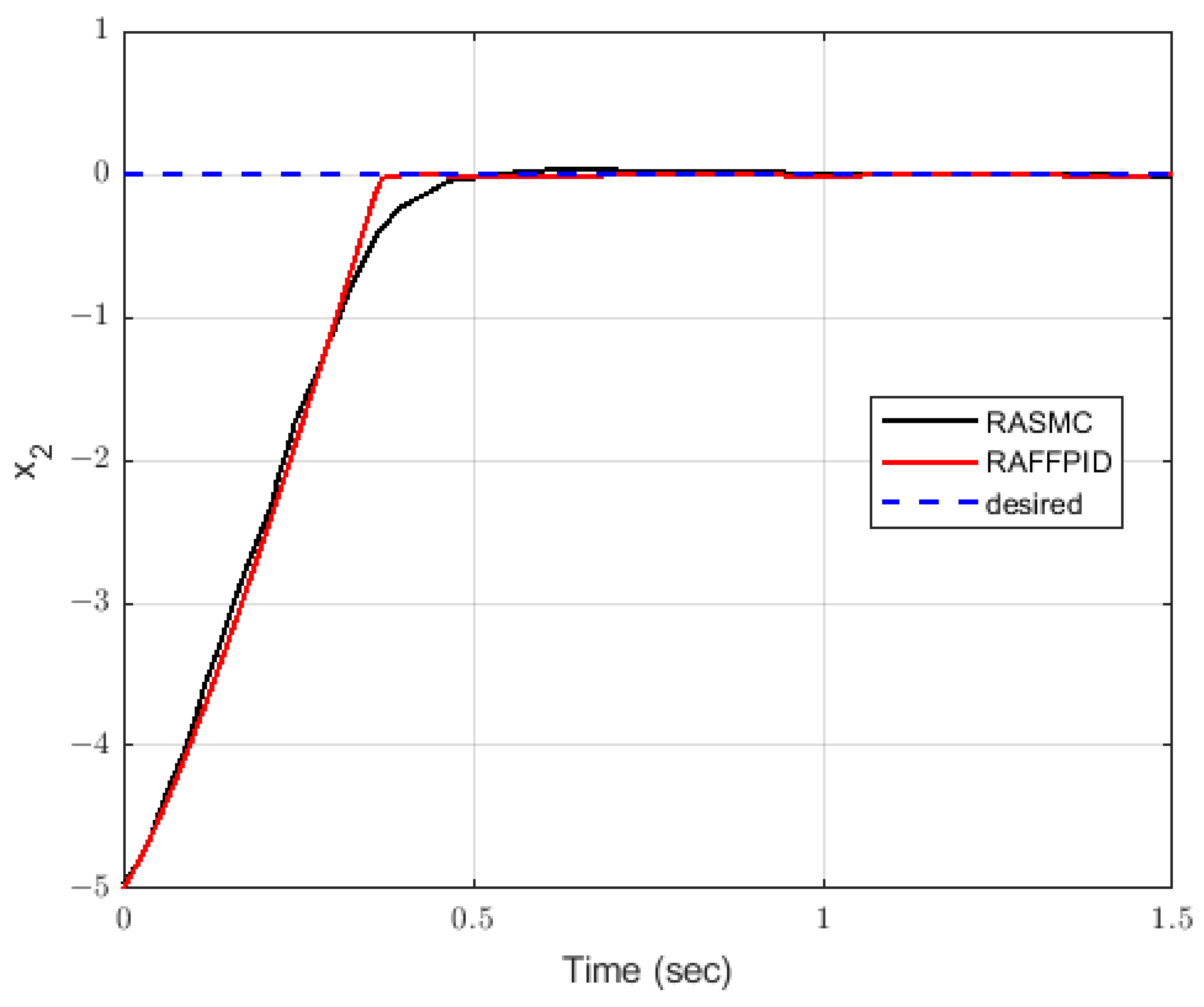
46] and robust adaptive sliding mode control [
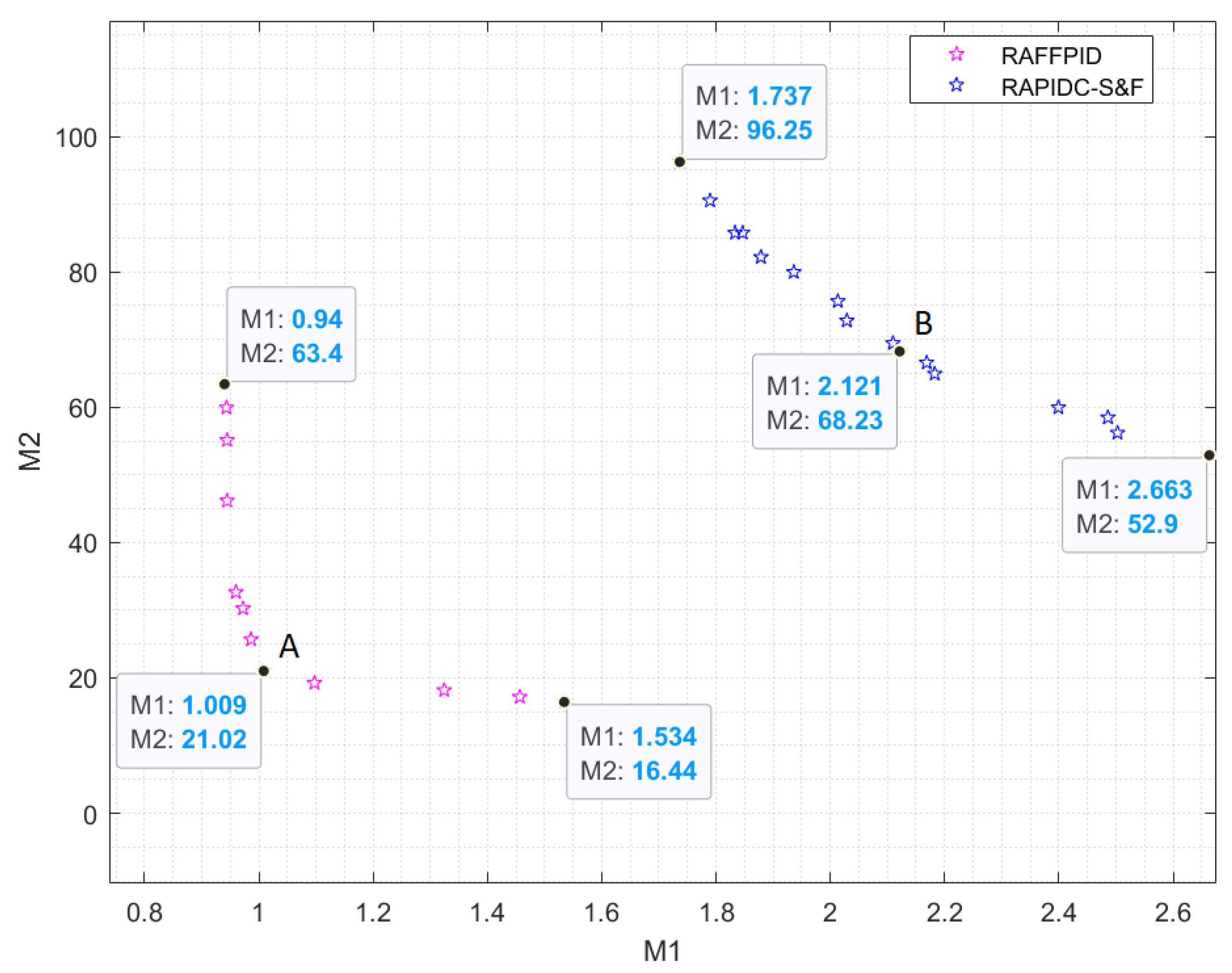
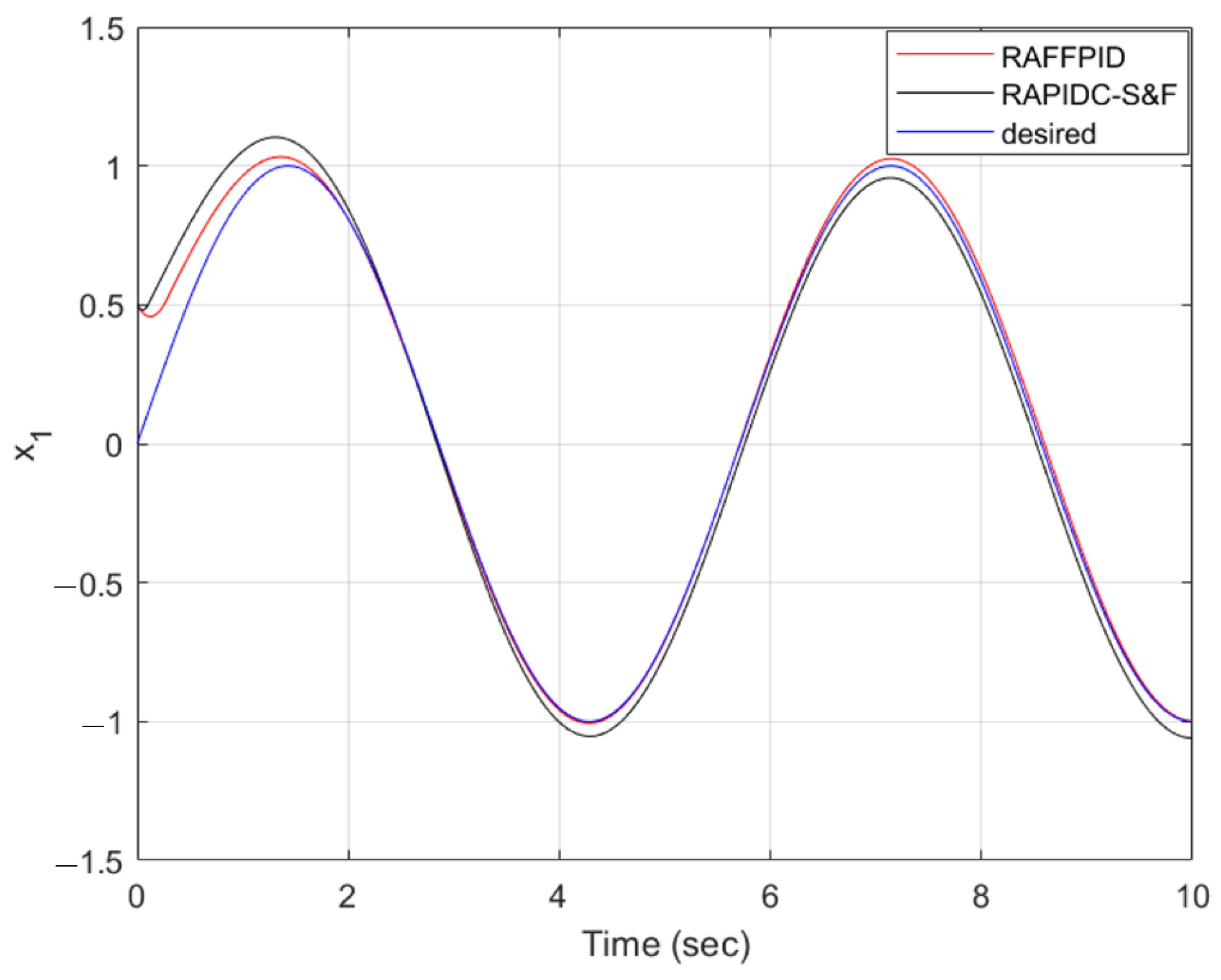
47] using a multi-objective optimization approach based on the genetic algorithm. The simulation results showed that the proposed controller outperformed the RAPIDC-S&F controller in reducing the values of the objective functions and providing a smoother control input. Moreover, the proposed controller demonstrated high effectiveness in reducing the values of the control effort and maintaining a smooth control input; its robustness was demonstrated against different input signals. Overall, this study provides strong evidence that the proposed controller is highly accurate and effective in controlling the system output.
Building upon these achievements, several exciting future research directions emerge. Firstly, extending the application of the RAFFPID controller to different chaotic systems with diverse dynamics and characteristics would provide a more comprehensive understanding of its effectiveness and generalizability. Secondly, exploring its practical implementation aspects, considering complexity, limitations, and real-time implementation constraints will ensure its broader applicability in real-world scenarios. Thirdly, considering the widely recognized effectiveness of the Takagi–Sugeno fuzzy model in approximating complex nonlinearities, it can be applied as an alternative to the conventional fuzzy model in the proposed controller presented in this paper. Additionally, investigating alternative optimization techniques and tuning approaches for the controller parameters could further enhance its performance, adaptability, and convergence speed. Furthermore, the proposed control strategy holds great potential for real-world applications in various domains, such as mechanical engineering, electronic circuit design, neuroscience, and beyond. Validating its performance on practical systems and evaluating its ability to handle uncertainties in real-world settings will contribute to its practicality and highlight its value in solving control problems in real-world scenarios.

Author Contributions

Conceptualization, M.J.M. and N.L.; Methodology, M.S.B., M.J.M. and N.L.; Validation, M.S.B. and M.J.M.; Formal analysis, N.L.; Investigation, M.J.M.; Resources, N.L.; Writing—original draft, M.S.B., M.J.M. and N.L.; Writing—review & editing, M.S.B., M.J.M. and N.L.; Visualization, M.S.B. and M.J.M.; Supervision, M.S.B.; Project administration, N.L.; Funding acquisition, N.L. All authors have read and agreed to the published version of the manuscript.

Funding

This research received no external funding.

Data Availability Statement

Data sharing not applicable.

Conflicts of Interest

The authors declare no conflict of interest.

Abbreviations

DescriptionNotation
External disturbanceD
Error vectorE
Error signale
System dynamicsf
System dynamics upper bound f u
System uncertaintiesg
System uncertainties upper Bound g u
Derivative constant gains k d
Integral, constant gains k i
Proportional constant gains k p
Objective function M i
Number of rulesN
Positive definite symmetric matrixP
Positive definite symmetric matrixQ
Regulation signal q r
Timet
Control signalu
Feedback linearization controlu*
Fractional-order PID compensator u F O P I D
Supervisory control u s
Lyapunov functionV
Positive Lyapunov function V e
Pre-specified parameter V M
State vector χ
System states x i
Actual outputy
Desired input vector Y d
Desired input y d
External disturbances α
Learning rate γ i
Order of fractional integration λ
Minimum eigenvalue of P λ m i n ( P )
Order of fractional differentiation μ
Input membership function μ A j
Final time τ

References

  1. Azar, A.T.; Vaidyanathan, S.; Ouannas, A. Fractional Order Control and Synchronization of Chaotic Systems; Springer: Berlin/Heidelberg, Germany, 2017; ISBN 9783319502496. [Google Scholar]
  2. Hua, C.; Guan, X. Adaptive Control for Chaotic Systems. Chaos Solitons Fractals 2004, 22, 55–60. [Google Scholar] [CrossRef]
  3. Ahn, C.K.; Jung, S.T.; Kang, S.K.; Joo, S.C. Adaptive H Synchronization for Uncertain Chaotic Systems with External Disturbance. Commun. Nonlinear Sci. Numer. Simul. 2010, 15, 2168–2177. [Google Scholar] [CrossRef]
  4. Feng, G.; Chen, G. Adaptive Control of Discrete-Time Chaotic Systems: A Fuzzy Control Approach. Chaos Solitons Fractals 2005, 23, 459–467. [Google Scholar] [CrossRef]
  5. Yin, C.; Zhong, S.M.; Chen, W.F. Design of Sliding Mode Controller for a Class of Fractional-Order Chaotic Systems. Commun. Nonlinear Sci. Numer. Simul. 2012, 17, 356–366. [Google Scholar] [CrossRef]
  6. Yu, Y.; Zhang, S. Adaptive Backstepping Synchronization of Uncertain Chaotic System. Chaos Solitons Fractals 2004, 21, 643–649. [Google Scholar] [CrossRef]
  7. Zhang, X. Robust Integral Sliding Mode Control for Uncertain Switched Systems under Arbitrary Switching Rules. Nonlinear Anal. Hybrid Syst. 2020, 37, 100900. [Google Scholar] [CrossRef]
  8. Pradhan, S.K.; Das, D.K. A Robust H Sliding Mode Control Design for Wind-Integrated Interconnected Power System with Time-Delay and Actuator Saturation. Sustain. Energy Grids Netw. 2020, 23, 100370. [Google Scholar] [CrossRef]
  9. Hu, Y.; Wang, H. Robust Tracking Control for Vehicle Electronic Throttle Using Adaptive Dynamic Sliding Mode and Extended State Observer. Mech. Syst. Signal Process. 2020, 135, 106375. [Google Scholar] [CrossRef]
  10. Ye, M.; Wang, H. Robust Adaptive Integral Terminal Sliding Mode Control for Steer-by-Wire Systems Based on Extreme Learning Machine. Comput. Electr. Eng. 2020, 86, 106756. [Google Scholar] [CrossRef]
  11. Zhou, H.; Wei, Z.; Zeng, Z.; Yu, C.; Yao, B.; Lian, L. Adaptive Robust Sliding Mode Control of Autonomous Underwater Glider with Input Constraints for Persistent Virtual Mooring. Appl. Ocean Res. 2020, 95, 102027. [Google Scholar] [CrossRef]
  12. Van, M.; Do, X.P. Optimal Adaptive Neural PI Full-Order Sliding Mode Control for Robust Fault Tolerant Control of Uncertain Nonlinear System. Eur. J. Control 2020, 54, 22–32. [Google Scholar] [CrossRef]
  13. Mahmoodabadi, M.J. An Optimal Robust Fuzzy Adaptive Integral Sliding Mode Controller Based upon a Multi-Objective Grey Wolf Optimization Algorithm for a Nonlinear Uncertain Chaotic System. Chaos Solitons Fractals 2023, 167, 113092. [Google Scholar] [CrossRef]
  14. Milbradt, D.M.C.; de Evald, P.J.D.O.; Hollweg, G.V.; Gründling, H.A. A Hybrid Robust Adaptive Sliding Mode Controller for Partially Modelled Systems: Discrete-Time Lyapunov Stability Analysis and Application. Nonlinear Anal. Hybrid Syst. 2023, 48, 101333. [Google Scholar] [CrossRef]
  15. Chiang, M.H.; Lin, H.T. The Force Control of a Novel Variable Rotational Speed Hydraulic Pump-Controlled System Using Adaptive Fuzzy Controller with Self-Tuning Fuzzy Sliding-Mode Compensation. IFAC Proc. Vol. 2011, 44, 968–973. [Google Scholar] [CrossRef] [Green Version]
  16. Kim, S.K. Self-Tuning Adaptive Feedback Linearizing Output Voltage Control for AC/DC Converter. Control Eng. Pract. 2015. [Google Scholar] [CrossRef]
  17. Tavakoli, A.R.; Seifi, A.R. Adaptive Self-Tuning PID Fuzzy Sliding Mode Control for Mitigating Power System Oscillations. Neurocomputing 2016, 218, 146–153. [Google Scholar] [CrossRef]
  18. Roman, R.C.; Precup, R.E.; Bojan-Dragos, C.A.; Szedlak-Stinean, A.I. Combined Model-Free Adaptive Control with Fuzzy Component by Virtual Reference Feedback Tuning for Tower Crane Systems. Procedia Comput. Sci. 2019, 162, 267–274. [Google Scholar] [CrossRef]
  19. Scheinker, A.; Gessner, S.; Emma, C.; Edelen, A.L. Adaptive Model Tuning Studies for Non-Invasive Diagnostics and Feedback Control of Plasma Wakefield Acceleration at FACET-II. Nucl. Instrum. Methods Phys. Res. Sect. A Accel. Spectrometers Detect. Assoc. Equip. 2020, 967, 163902. [Google Scholar] [CrossRef]
  20. Borges, A.S.; Montano, I.D.C.; Sousa Junior, R.; Suarez, C.A.G. Automatic Solids Feeder Using Fuzzy Control: A Tool for Fed Batch Bioprocesses. J. Process Control 2020, 93, 28–42. [Google Scholar] [CrossRef]
  21. Masoumi, A.P.; Tavakolpour-Saleh, A.R.; Rahideh, A. Applying a Genetic-Fuzzy Control Scheme to an Active Free Piston Stirling Engine: Design and Experiment. Appl. Energy 2020, 268, 115045. [Google Scholar] [CrossRef]
  22. Jin, X.; Chen, K.; Zhao, Y.; Ji, J.; Jing, P. Simulation of Hydraulic Transplanting Robot Control System Based on Fuzzy PID Controller. Measurement 2020, 164, 108023. [Google Scholar] [CrossRef]
  23. Abbasi, S.M.M.; Jalali, A. Fuzzy Tracking Control of Fuzzy Linear Dynamical Systems. ISA Trans. 2020, 97, 102–115. [Google Scholar] [CrossRef] [PubMed]
  24. Deng, Y.; Zhang, X.; Zhang, Q.; Hu, Y. Event-Triggered Composite Adaptive Fuzzy Control of Sailboat with Heeling Constraint. Ocean Eng. 2020, 211, 107627. [Google Scholar] [CrossRef]
  25. Nejadkourki, N.; Mahmoodabadi, M.J. Fuzzy Adaptive State-Feedback Control for a Revolute-Prismatic-Revolute Robot Manipulator. Cogent Eng. 2019, 6, 1698690. [Google Scholar] [CrossRef]
  26. Bahraini, S.M.S.; Eghtesad, M.; Farid, M. Application of Fractional-Order Control for Vibration Suppression of Viscoelastic Beams. Int. J. Comput. Mater. Sci. Eng. 2014, 3, 1450006. [Google Scholar] [CrossRef]
  27. Jajarmi, A.; Baleanu, D. Suboptimal Control of Fractional-Order Dynamic Systems with Delay Argument. J. Vib. Control 2018, 24, 2430–2446. [Google Scholar] [CrossRef]
  28. Agarwal, R.P.; Baleanu, D.; Nieto, J.J.; Torres, D.F.M.; Zhou, Y. A Survey on Fuzzy Fractional Differential and Optimal Control Nonlocal Evolution Equations. J. Comput. Appl. Math. 2018, 339, 3–29. [Google Scholar] [CrossRef] [Green Version]
  29. Ma, T. Filtering Adaptive Output Feedback Control for Multivariable Nonlinear Systems with Mismatched Uncertainties and Unmodeled Dynamics. Int. J. Robust Nonlinear Control 2020, 30, 8007–8028. [Google Scholar] [CrossRef]
  30. Zhu, B.; Wang, Y.; Zhang, H.; Xie, X. Fuzzy Functional Observer-Based Finite-Time Adaptive Sliding Mode Control for Nonlinear Systems with Matched Uncertainties. IEEE Trans. Fuzzy Syst. 2021, 30, 918–932. [Google Scholar] [CrossRef]
  31. Cattani, C.; Srivastava, H.M.; Yang, X.J. Fractional Dynamics; Walter de Gruyter GmbH & Co KG: Berlin, Germany, 2015; ISBN 9783110472097. [Google Scholar]
  32. Bahraini, S.M.S.; Eghtesad, M.; Farid, M.; Ghavanloo, E. Large Deflection of Viscoelastic Beams Using Fractional Derivative Model. J. Mech. Sci. Technol. 2013, 27, 1063–1070. [Google Scholar] [CrossRef]
  33. Bahraini, S.M.S.; Eghtesad, M.; Farid, M.; Ghavanloo, E. Analysis of an Electrically Actuated Fractional Model of Viscoelastic Microbeams. Struct. Eng. Mech. 2014, 52, 937–956. [Google Scholar] [CrossRef]
  34. Mainardi, F. Fractional Calculus and Waves in Linear Viscoelasticity; World Scientific: Singapore, 2021. [Google Scholar]
  35. Yang, Q.; Chen, D.; Zhao, T.; Chen, Y. Fractional Calculus in Image Processing: A Review. Fract. Calc. Appl. Anal. 2016, 19, 1222–1249. [Google Scholar] [CrossRef] [Green Version]
  36. Sayevand, K.; Yazdani, A.; Arjang, F. Cubic B-Spline Collocation Method and Its Application for Anomalous Fractional Diffusion Equations in Transport Dynamic Systems. J. Vib. Control 2016, 22, 2173–2186. [Google Scholar] [CrossRef]
  37. Magin, R.L. Fractional Calculus in Bioengineering. Crit. Rev. Biomed. Eng. 2004, 32. [Google Scholar]
  38. Zhang, X.; Li, D.; Zhang, X. Adaptive Impulsive Synchronization for a Class of Fractional Order Complex Chaotic Systems. J. Vib. Control 2019, 25, 1614–1628. [Google Scholar] [CrossRef]
  39. Abouelregal, A.E. Thermoelastic Fractional Derivative Model for Exciting Viscoelastic Microbeam Resting on Winkler Foundation. J. Vib. Control 2020, 27, 2123–2135. [Google Scholar] [CrossRef]
  40. Shah, P.; Agashe, S. Review of Fractional PID Controller. Mechatronics 2016, 38, 29–41. [Google Scholar] [CrossRef]
  41. Dastjerdi, A.A.; Vinagre, B.M.; Chen, Y.Q.; HosseinNia, S.H. Linear Fractional Order Controllers; A Survey in the Frequency Domain. Annu. Rev. Control 2019, 47, 51–70. [Google Scholar] [CrossRef]
  42. Kumari, S.; Raj, S.; Kumar, R. Performance Review of Fractional Order PID (FOPID) Based Controllers Employed in Brushless DC Motor. In Proceedings of the 2020 International Conference on Power Electronics & IoT Applications in Renewable Energy and Its Control (PARC), Mathura, India, 28–29 February 2020. [Google Scholar]
  43. Zirkohi, M.M. Robust Adaptive Backstepping Control of Uncertain Fractional-Order Nonlinear Systems with Input Time Delay. Math. Comput. Simul. 2022, 196, 251–272. [Google Scholar] [CrossRef]
  44. Liu, F.; Zhang, X. Compound Adaptive Fuzzy Synchronization Controller Design for Uncertain Fractional-Order Chaotic Systems. Fractal Fract. 2022, 6, 652. [Google Scholar] [CrossRef]
  45. Mok, R.; Ahmad, M.A. Fast and optimal tuning of fractional order PID controller for AVR system based on memorizable-smoothed functional algorithm. Eng. Sci. Technol. Int. 2022, 35, 101264. [Google Scholar] [CrossRef]
  46. Mahmoodabadi, M.J.; Abedzadeh Maafi, R.; Taherkhorsandi, M. An Optimal Adaptive Robust PID Controller Subject to Fuzzy Rules and Sliding Modes for MIMO Uncertain Chaotic Systems. Appl. Soft Comput. J. 2017, 52, 1191–1199. [Google Scholar] [CrossRef]
  47. Thanh, H.L.; Vu, M.T.; Nguyen, N.P.; Mung, N.X.; Hong, S.K. Finite-time stability of MIMO nonlinear systems based on robust adaptive sliding control: Methodology and application to stabilize chaotic motions. IEEE Access. 2021, 9, 21759–21768. [Google Scholar] [CrossRef]
Figure 1. Block diagram of the proposed RAFFPID controller.
Fractalfract 07 00484 g001
Figure 2. Triangular membership functions used for the inputs of the fuzzy systems.
Fractalfract 07 00484 g002
Figure 3. Comparison between the Pareto fronts of RAFFPID and RAPIDC-S&F [46] for the initial condition, x 1 ( 0 ) = 0.2, and x 2 ( 0 ) = 0.2.
Fractalfract 07 00484 g003
Figure 4. Comparison between the Pareto fronts of RAFFPID and RAPIDC-S&F [46] for the initial condition, x 1 ( 0 ) = 0.5, and x 2 ( 0 ) = −0.7.
Fractalfract 07 00484 g004
Figure 5. Comparison of the trajectory tracking for state x 1 ( t ) for the proposed controller and the RAPIDC-S&F [46]—the initial conditions are chosen as x 1 ( 0 ) = 0.5 and x 2 ( 0 ) = −0.7.
Fractalfract 07 00484 g005
Figure 6. Comparison of the trajectory tracking for state x 2 ( t ) obtained by the proposed controller and the RAPIDC-S&F [46] the initial conditions are chosen as x 1 ( 0 ) = 0.5 and x 2 ( 0 ) = −0.7.
Fractalfract 07 00484 g006
Figure 7. Comparison of the control inputs obtained by the proposed controller and the RAPIDC-S&F [46] the initial conditions are chosen as x 1 ( 0 ) = 0.5 and x 2 ( 0 ) = −0.7.
Fractalfract 07 00484 g007
Figure 8. Comparison of the trajectory tracking for state x 1 ( t ) for the proposed controller and the RAPIDC-S&F [46] for the square waves.
Fractalfract 07 00484 g008
Figure 9. Comparison of the trajectory tracking for state x 2 ( t ) for the proposed controller and the RAPIDC-S&F [46] for the square waves.
Fractalfract 07 00484 g009
Figure 10. Comparison of the trajectory tracking for state x 1 ( t ) for the proposed controller (RAFFPID) and RASMC.
Fractalfract 07 00484 g010
Figure 11. Comparison of the trajectory tracking for state x 2 ( t ) for the proposed controller (RAFFPID) and RASMC.
Fractalfract 07 00484 g011
Table 1. Fuzzy rule base for the learning rate parameters.
AntecedentsConsequents
e   is   μ A 1 γ i f = 1
e   is   μ A 2 γ i f = 0
e   is   μ A 3 γ i f = + 1
Disclaimer/Publisher’s Note: The statements, opinions and data contained in all publications are solely those of the individual author(s) and contributor(s) and not of MDPI and/or the editor(s). MDPI and/or the editor(s) disclaim responsibility for any injury to people or property resulting from any ideas, methods, instructions or products referred to in the content.

