Interpolated Coefficient Mixed Finite Elements for Semilinear Time Fractional Diffusion Equations

Abstract

In this paper, we consider a fully discrete interpolated coefficient mixed finite element method for semilinear time fractional reaction–diffusion equations. The classic $L1$ scheme based on graded meshes and new mixed finite element based on triangulation is used for the temporal and spatial discretization, respectively. The interpolation coefficient technique is used to deal with the semilinear term, and the discrete nonlinear system is solved by a Newton-like iterative method. Stability and convergence results for both the original variable and its flux are derived. Numerical experiments confirm our theoretical analysis.

1. Introduction

Time fractional partial differential equations (FPDEs) are broadly used to describe some phenomena or processes with memory and heritability in different fields, such as ecology, biology, finance, chemistry, physics and engineering [1]. Since most of the FPDEs cannot be analytically solved [2], many numerical methods have been proposed for FPDEs. A systematic introduction can be found in [3,4] and the references therein.

There are mainly three kinds of FPDEs, namely, time FPDEs, space FPDEs and time-space FPDEs. In the last few decades, many numerical methods, such as the spectral method [5], finite difference method [6,7], finite element method (FEM) [8,9], mixed finite element method (MFEM) [10,11], space-time FEM [12], discontinuous Galerkin FEM [13], finite volume method [14], virtual element method [15], fast algorithms based on the sum-of-exponential approximation [16,17,18] and higher-order schemes [19,20] have been developed for time FPDEs, mostly focused on the linear case. Recently, there have also been a few works on the nonlinear time FPDEs [21,22,23,24].

For FEMs solving nonlinear partial differential equations, Xu presented a two-grid FEM for nonlinear elliptic equations in [25], and Zlámal and Larsson provided an interpolated coefficient (IC) FEM for nonlinear parabolic equations in [26,27]. The IC technique is a simple and graceful idea. It not only simplifies the calculation of the numerical integration of nonlinear terms, but also facilitates the solution of the corresponding discrete nonlinear system. Recently, IC has been extended to solve some nonlinear equations [28].

The Ladyženskaja-Babuška-Brezzi (LBB) condition must be satisfied between the discrete space pairs used in classic MFEM, for example, $P_k^2-x{P}_{k-1}$ Ravairt-Thomas MFEM. This results in little available space pairs and huge computational costs. In order to be free of the LBB condition, Pani proposed an $H^1$-Galerkin MFEM in [29] and Yang presented a splitting positive definite MFEM in [30]. In 2010, Chen developed a new $P_{k-1}^2-P_k$ MFEM in [31]. Compared to $P_k^2-x{P}_{k-1}$ Ravairt-Thomas MFEM, this method has two main advantages: one is the lower regularity requirement of the equation; the other is the lower computational cost. In recent years, it has been used to solve parabolic equations [32].

In this article, we will propose a fully discrete interpolated coefficient $P_{k-1}^2-P_k$ mixed finite element (ICPMFE) approximation for semilinear time fractional reaction–diffusion equations (STFRDEs) by combining the advantages of IC and $P_{k-1}^2-P_k$ MFEM. The stability and convergence results for all variables will be derived. The STFRDEs can be derived from the continuous time random walk model with temporal memory and sources or population model [33,34,35]. Compared with the general reaction–diffusion models, the STFRDEs have a fractional derivative index and exhibit self-organization phenomena.

We are interested in the following STFRDE:

$$\begin{array}{cc}\hfill & {\mathcal{D}}_t^{\alpha }u-\mathit{div}(A\nabla u)+\varphi (u)=f,x\in \Omega ,t\in J,\hfill \end{array}$$

(1)

$$\begin{array}{cc}\hfill & u(x,t)=0,x\in \partial \Omega ,t\in \overline{J},\hfill \end{array}$$

(2)

$$\begin{array}{cc}\hfill & u(x,0)=u_0(x),x\in \Omega ,\hfill \end{array}$$

(3)

where $\Omega \subset R^2$ is a convex polygonal domain with boundary $\partial \Omega$, $J=(0,T]$, and $D_t^{\alpha }$ denotes the $\alpha$-order $(0<\alpha <1)$ left Caputo derivative [1], namely

$$\begin{array}{c}\hfill {\mathcal{D}}_t^{\alpha }u(·,t)=\frac{1}{\Gamma (1-\alpha )}{\int }_0^t\frac{\partial u(·,s)}{\partial s}\frac{1}{{(t-s)}^{\alpha }}ds.\end{array}$$

$A=A(x)={(a_{ij}(x))}_{2\times 2}\in W^{2,\infty }{(\overline{\Omega })}^{2\times 2}$ satisfies $c_{*}{\parallel \xi \parallel }^2\le {\xi }^{\mathsf{T}}A\xi \le c^{*}{\parallel \xi \parallel }^2,\forall \xi \in R^2$ with $c_{*},c^{*}>0$. $\varphi (·)$, $f(x,t)\in L^2(J;L^2(\Omega ))$ and $u_0(x)\in H^1(\Omega )$ are known real-valued functions, there is constant $M>0$ such that

$$|\varphi (u)|\le M\left|u\right|,$$

and

$${\varphi }^{\prime }(·)\ge 0,|{\varphi }^{\prime }(·)|+|{\varphi }^{″}(·)|\le M.$$

Moreover, we assume (1)–(3) has a solution $u(x,t)$, which satisfies condition [16]

$$\begin{array}{c}\hfill \left|\frac{{\partial }^{k}u(x,t)}{\partial t^k}\right|\le c_0{t}^{\alpha -k},0\le k\le 3,\end{array}$$

(4)

where $c_0$ is a positive constant, which depends on the problem but not on the mesh parameters h and $\tau$.

In this paper, we denote the Sobolev space on $\Omega$ as $W^{m,p}(\Omega )$ with a semi-norm ${|·|}_{m,p}$ and a norm ${\parallel ·\parallel }_{m,p}$ given by ${\left|w\right|}_{m,p}=({\sum }_{\beta =m}\parallel D^{\beta }w{{\parallel }_{L^p(\Omega )}^p)}^{1/p}$ and ${\parallel w\parallel }_{m,p}=({\sum }_{\beta \le m}\parallel D^{\beta }w{{\parallel }_{L^p(\Omega )}^p)}^{1/p}$, respectively. When $p=2$, we set $H^m(\Omega )=W^{m,2}(\Omega )$, $H_0^1(\Omega )=\{v\in H^1(\Omega ):v{|}_{\partial \Omega }=0\}$, ${\parallel ·\parallel }_m={\parallel ·\parallel }_{m,2}$ and $\parallel ·\parallel ={\parallel ·\parallel }_{0,2}$. Moreover, C is a generic positive constant independent of mesh parameters h and $\tau$.

The plan of this paper is as follows. A fully discrete ICPMFE approximation scheme of (1)–(3) is given in Section 2. An unconditional stability is presented in Section 3. Convergence results are established in Section 4. Two numerical examples are conducted to confirm our theoretical findings in Section 5.

2. A Fully Discrete ICPMFE Approximation

We shall construct a fully discrete ICPMFE approximation of (1)–(3) in this section. For simplicity of presentation, we set $U=L^2(\Omega )$, $W=H_0^1(\Omega )$, $\mathit{V}={(L^2(\Omega ))}^2$, $\mathit{H}=H(\mathit{div};\Omega )=\left\{\mathit{v}\in \mathit{V},\mathit{div}\mathit{v}\in L^2(\Omega )\right\}$ and the corresponding $L^2$-inner product $(·,·)$ is defined as follows:   

$$\begin{array}{cc}\hfill & (f_1,f_2)={\int }_{\Omega }{f}_1{f}_2,\forall f_1,f_2\in U,\hfill \\ \hfill & (\mathit{\phi },\mathit{\psi })=\sum _{i=1}^2({\mathit{\phi }}_i,{\mathit{\psi }}_i),\forall \mathit{\phi },\mathit{\psi }\in \mathit{V}.\hfill \end{array}$$

Let $\mathcal{A}=A^{-1}$ and $\mathit{p}=A\nabla u$. Like in [36], we derive the classical mixed weak form of (1)–(3) as: Find $\{\mathit{p},u\}:[0,T]\mapsto \mathit{H}\times U$, such that

$$\begin{array}{cc}\hfill & \left({\mathcal{D}}_t^{\alpha }u,w\right)-(\nabla \mathit{p},w)+(\varphi (u),w)=(f,w),\forall w\in U,\hfill \end{array}$$

(5)

$$\begin{array}{cc}\hfill & (\mathcal{A}\mathit{p},\mathit{v})+(u,\nabla ·\mathit{v})=0,\forall \mathit{v}\in \mathit{H}.\hfill \end{array}$$

(6)

$$\begin{array}{cc}\hfill & u(x,0)=u_0(x),\forall x\in \Omega .\hfill \end{array}$$

(7)

Similar to [31], we derive a new mixed variational form of (1)–(3) as: Find $\{\mathit{p},u\}:[0,T]\mapsto \mathit{V}\times W$, such that

$$\begin{array}{cc}\hfill & \left({\mathcal{D}}_t^{\alpha }u,w\right)+(\mathit{p},\nabla w)+(\varphi (u),w)=(f,w),\forall w\in W,\hfill \end{array}$$

(8)

$$\begin{array}{cc}\hfill & (\mathcal{A}\mathit{p},\mathit{v})-(\nabla u,\mathit{v})=0,\forall \mathit{v}\in \mathit{V}.\hfill \end{array}$$

(9)

$$\begin{array}{cc}\hfill & u(x,0)=u_0(x),\forall x\in \Omega .\hfill \end{array}$$

(10)

Remark 1.

Compared with the classical mixed weak form (5)–(7), there are two advantages of the new mixed weak form (8)–(10). One is the flux $\mathit{p}\in \mathit{V}$ and the other is that it avoids the use of the complex space $\mathit{H}$.

2.1. The Temporal Discretization

The graded temporal mesh is ${\{t_n=T{(n/N)}^r\}}_{n=0}^N$, $N\in {\mathbb{Z}}^{+}$, where $r\ge 1$. Set $u(x,t_n)=u^n$, ${\tau }_n=t_n-t_{n-1}$, $n=1,2,\cdots ,N$ and $\tau =max{\left\{{\tau }_n\right\}}_{n=1}^N$. Then the $L1$ discrete scheme of the Caputo derivative is as follows [7,37]: For $n=1,2,\cdots ,N$,

$$\begin{array}{c}\hfill \begin{array}{cc}\hfill {\mathcal{D}}_t^{\alpha }{u}^n& =\frac{1}{\Gamma (1-\alpha )}\sum _{k=0}^{n-1}\frac{u^{k+1}-u^k}{{\tau }_{k+1}}{\int }_{t_k}^{t_{k+1}}\frac{ds}{{(t_n-s)}^{\alpha }}+R_u^n\hfill \\ \hfill & =\frac{1}{\Gamma (2-\alpha )}\sum _{k=0}^{n-1}\frac{u^{k+1}-u^k}{{\tau }_{k+1}}\left[{(t_n-t_k)}^{1-\alpha }-{(t_n-t_{k+1})}^{1-\alpha }\right]+R_u^n\hfill \\ \hfill & =\frac{1}{\Gamma (2-\alpha )}\sum _{k=1}^{n-1}(d_{n,k+1}-d_{n,k})u^{n-k}-\frac{d_{n,1}}{\Gamma (2-\alpha )}{u}^n-\frac{d_{n,n}}{\Gamma (2-\alpha )}{u}^0+R_u^n\hfill \\ \hfill & :={\mathcal{D}}_N^{\alpha }{u}^n+R_u^n,\hfill \end{array}\end{array}$$

(11)

where $d_{n,1}={\tau }_n^{-\alpha }$ and

$$d_{n,k}=\frac{{(t_n-t_{n-k})}^{1-\alpha }-{(t_n-t_{n-k+1})}^{1-\alpha }}{{\tau }_{n-k+1}},k=1,2,\cdots ,n.$$

If $|u^{″}(t)|\le C{t}^{\alpha -2},0\le t\le T$, it follows from [18] that the truncation error is bounded by

$$\begin{array}{c}\hfill |R_u^n|:=|{\mathcal{D}}_t^{\alpha }{u}^n-{\mathcal{D}}_N^{\alpha }{u}^n|\le C{n}^{-min\{2-\alpha ,r(1+\alpha )\}},n=1,2,\cdots ,N.\end{array}$$

(12)

2.2. The Spatial Discretization

Let ${\mathcal{T}}_h$ be regular triangulations of $\Omega$. $h_e$ denotes the diameter of e and $h=\underset{e\in {\mathcal{T}}_h}{max}\left\{h_e\right\}$. $P_k$ is a polynomial space of total degree up to k. Let ${\mathit{V}}_h\times W_h\subset \mathit{V}\times W$ be defined by the following finite element pairs $P_{k-1}^2-P_k$ [31]:   

$$\begin{array}{cc}\hfill & {\mathit{V}}_h=\{{\mathit{v}}_h=(v_{1h},v_{2h})\in \mathit{V}:v_{ih}{|}_e\in P_{k-1}(e),\forall e\in {\mathcal{T}}_h,i=1,2\},\hfill \\ \hfill & W_h=\{w_h\in C^0(\overline{\Omega })\cap W:w_h{|}_e\in P_k(e),\forall e\in {\mathcal{T}}_h\}.\hfill \end{array}$$

Then, a fully discrete MFEM approximation of (1)–(3) is: Find $({\mathit{p}}_h^n,u_h^n)\in {\mathit{V}}_h\times W_h,$$n=1,2,\cdots ,N$, such that

$$\begin{array}{cc}\hfill & \left({\mathcal{D}}_N^{\alpha }{u}_h^n,w_h\right)+({\mathit{p}}_h^n,\nabla w_h)+(\varphi (u_h^n),w_h)=(f^n,w_h),\forall w_h\in W_h,\hfill \end{array}$$

(13)

$$\begin{array}{cc}\hfill & (\mathcal{A}{\mathit{p}}_h^n,{\mathit{v}}_h)-(\nabla u_h^n,{\mathit{v}}_h)=0,\forall {\mathit{v}}_h\in {\mathit{V}}_h,\hfill \end{array}$$

(14)

$$\begin{array}{cc}\hfill & u_h^0=P_h{u}_0,\hfill \end{array}$$

(15)

where projection $P_h$ will be specified later.

Let ${\left\{{\phi }_i\right\}}_{i=1}^{M_1}$ be the element-basis functions of discrete space $W_h$. Then, numerical solution $u_h^n\in W_h$ can be expressed as $u_h^n=\sum _{i=1}^{M_1}{u}_{h,i}^n{\phi }_i$. Set ${\left\{{\mathit{\psi }}_i\right\}}_{i=1}^{M_2}$ as the edge-basis functions of discrete space ${\mathit{V}}_h$. Then, we can assume ${\mathit{p}}_h^n=\sum _{i=1}^{M_2}{\mathit{p}}_{h,i}^n·{\mathit{\psi }}_i$. By selecting $w_h={\phi }_i,i=1,2,\cdots ,M_1$ in (13), we obtain the following nonlinear system:

$$\begin{array}{c}\hfill {\mathcal{D}}_N^{\alpha }\left[\sum _{j=1}^{M_1}({\phi }_j,{\phi }_i)u_{h,j}^n\right]+\sum _{j=1}^{M_2}\left({\mathit{\psi }}_j·{\mathit{p}}_{h,j}^n,\nabla {\phi }_i\right)+\left(\varphi \left(\sum _{j=1}^{M_1}{u}_{h,j}^n{\phi }_j\right),{\phi }_i\right)=(f^n,{\phi }_i),\end{array}$$

(16)

which is often solved by the Newton-like method. Its main concern is to compute the Jacobi matrix. The Jacobi matrix of (16) is as follows:

$$\begin{array}{c}\hfill {\mathcal{D}}_N^{\alpha }\left[\sum _{j=1}^{M_1}({\phi }_j,{\phi }_i)\right]+\sum _{j=1}^{M_2}\left({\mathit{\psi }}_j,\nabla {\phi }_i\right)+\left({\varphi }^{\prime }\left(\sum _{k=1}^{M_1}{u}_{h,k}^n{\phi }_k\right){\phi }_j,{\phi }_i\right)=0,i=1,2,\cdots ,M_1.\end{array}$$

(17)

It depends on the choice of $u_h^n$, and needs to repeatedly compute as the iterations proceed. Obviously, the integration of the semilinear term in (17) will result in the very time-consuming and expensive computation.

We introduce an interpolation operator $I_h:W\to W_h$ [27], which satisfies: For any $\vartheta \in W$,

$$I_h\vartheta =\sum _{i=1}^{M_1}{\vartheta }_i{\phi }_i.$$

The following error estimate is valid [27]: For $0\le r\le k+1$ and $1\le p\le \infty$,

$$\begin{array}{c}\hfill \parallel \vartheta -I_h{\vartheta \parallel }_{r,p}\le C{h}^{k+1-r}{\parallel \mathit{\psi }\parallel }_{k+1,p},\forall \vartheta \in C(\overline{\Omega })\cap W^{k+1,p}(\tau ),\forall \tau \in {\mathcal{T}}^h.\end{array}$$

(18)

Then, a fully discrete ICPMFE approximation of (1)–(3) is: Find $({\mathit{p}}_h^n,u_h^n)\in {\mathit{V}}_h\times W_h,n=1,2,\cdots ,N$, such that

$$\begin{array}{cc}\hfill & \left({\mathcal{D}}_N^{\alpha }{u}_h^n,w_h\right)+({\mathit{p}}_h^n,\nabla w_h)+(I_h\varphi (u_h^n),w_h)=(f^n,w_h),\forall w_h\in W_h,\hfill \end{array}$$

(19)

$$\begin{array}{cc}\hfill & (\mathcal{A}{\mathit{p}}_h^n,{\mathit{v}}_h)-(\nabla u_h^n,{\mathit{v}}_h)=0,\forall {\mathit{v}}_h\in {\mathit{V}}_h,\hfill \end{array}$$

(20)

$$\begin{array}{cc}\hfill & u_h^0=P_h{u}_0.\hfill \end{array}$$

(21)

By taking $w_h={\phi }_i,i=1,2,\cdots ,M_1$ in (19), we obtain the following nonlinear system:

$$\begin{array}{c}\hfill {\mathcal{D}}_N^{\alpha }\left[\sum _{j=1}^{M_1}({\phi }_j,{\phi }_i)u_{h,j}^n\right]+\sum _{j=1}^{M_2}\left({\mathit{\psi }}_j·{\mathit{p}}_{h,j}^n,\nabla {\phi }_i\right)+\sum _{j=1}^{M_1}\varphi (u_{h,j}^n)({\phi }_j,{\phi }_i)=(f^n,{\phi }_i).\end{array}$$

(22)

Its Jacobi matrix is as follows:

$$\begin{array}{cc}\hfill & {\mathcal{D}}_N^{\alpha }\left[\sum _{j=1}^{M_1}({\phi }_j,{\phi }_i)\right]+\sum _{j=1}^{M_2}\left({\mathit{\psi }}_j,\nabla {\phi }_i\right)+\sum _{j=1}^{M_1}{\varphi }^{\prime }(u_{h,j}^n)({\phi }_j,{\phi }_i)=0,i=1,2,\cdots ,M_1.\hfill \end{array}$$

(23)

For example, let $\varphi (u)=u^3$, then ${\varphi }^{\prime }(u)=3u^2$. The semilinear term in (17) is

$$\begin{array}{c}\hfill \left({\varphi }^{\prime }\left(\sum _{k=1}^{M_1}{u}_{h,k}^n{\phi }_k\right){\phi }_j,{\phi }_i\right)=3\left({\left(\sum _{k=1}^{M_1}{u}_{h,k}^n{\phi }_k\right)}^2{\phi }_j,{\phi }_i\right)=3\sum _{k,l=1}^{M_1}{u}_{h,k}^n{u}_{h,l}^n\left({\phi }_k{\phi }_l{\phi }_j,{\phi }_i\right),\end{array}$$

whereas the semilinear term in (23) is

$$\begin{array}{c}\hfill \sum _{j=1}^{M_1}{\varphi }^{\prime }(u_{h,j}^n)({\phi }_j,{\phi }_i)=3\sum _{j=1}^{M_1}{(u_{h,j}^n)}^2({\phi }_j,{\phi }_i).\end{array}$$

Hence, the integration of the semilinear term in (23) is reduced greatly compared with (17).

3. Stability Analysis

The following conclusions will be needed in the subsequent stability analysis.

Lemma 1 ([38]).

Let the functions $v_j=v(·,t_j)$ be in $L^2(\Omega )$ for $j=0,1,\cdots ,N$. Then, the discrete $L1$ scheme described as (11) satisfies

$$\begin{array}{c}\hfill \left({\mathcal{D}}_N^{\alpha }{v}^n,v^n\right)\ge \left({\mathcal{D}}_N^{\alpha }\parallel v^n\parallel \right)\parallel v^n\parallel ,n=1,2,\cdots ,N.\end{array}$$

(24)

Lemma 2 ([39]).

Assume that the sequences ${\left\{{\xi }^n\right\}}_{n=1}^N$ and ${\left\{{\sigma }^n\right\}}_{n=1}^N$ are nonnegative, that $V^0\ge 0$, and that the sequences ${\left\{V^n\right\}}_{n=1}^N$ satisfy

$$V^n{\mathcal{D}}_N^{\alpha }{V}^n\le {\xi }^n{V}^n+{({\sigma }^n)}^2,n=1,2,\cdots ,N.$$

Then

$$\begin{array}{c}\hfill V^N\le V^0+\Gamma (1-\alpha )\underset{j=1,2,\cdots ,n}{max}{t}_j^{\alpha }{\xi }^j+\sqrt{\Gamma (1-\alpha )}\underset{j=1,2,\cdots ,n}{max}{t}_j^{\frac{\alpha }{2}}{\sigma }^j,n=1,2,\cdots ,N.\end{array}$$

(25)

We now show the uncondition stability of (19)–(21).

Theorem 1.

For $n=1,2,\cdots ,N$, we assume $(u_h^n,{\mathit{p}}_h^n)$ is the solution of (19)–(21). Then

$$\begin{array}{cc}\hfill & \parallel u_h^n\parallel \le C\left(\parallel u_h^0\parallel +\underset{0\le i\le N}{max}\parallel f^j\parallel \right),\hfill \end{array}$$

(26)

$$\begin{array}{cc}\hfill & \parallel {\mathit{p}}_h^n\parallel \le C\left(\parallel {\mathit{p}}_h^0\parallel +\underset{0\le i\le N}{max}\parallel f^j\parallel \right).\hfill \end{array}$$

(27)

Proof. 

Choosing $w_h=u_h^n$ in (19) and ${\mathit{v}}_h=\nabla u_h^n$ in (20), we have

$$\begin{array}{cc}\hfill & \left({\mathcal{D}}_N^{\alpha }{u}_h^n,u_h^n\right)+({\mathit{p}}_h^n,\nabla u_h^n)+(I_h\varphi (u_h^n),u_h^n)=(f^n,u_h^n),\hfill \end{array}$$

(28)

$$\begin{array}{cc}\hfill & (\mathcal{A}{\mathit{p}}_h^n,\nabla u_h^n)-(\nabla u_h^n,\nabla u_h^n)=0.\hfill \end{array}$$

(29)

Substitute (29) into (28), we get

$$\begin{array}{c}\hfill \left({\mathcal{D}}_N^{\alpha }{u}_h^n,u_h^n\right)+(A\nabla u_h^n,\nabla u_h^n)=(f^n,u_h^n)-(I_h\varphi (u_h^n),u_h^n).\end{array}$$

(30)

From Lemma 1, we have $\left({\mathcal{D}}_N^{\alpha }\parallel u_h^n\parallel \right)\parallel u_h^n\parallel \le \left({\mathcal{D}}_N^{\alpha }{u}_h^n,u_h^n\right)$. According to the assumptions on A, it is easy to see $c\parallel \nabla u_h^n{\parallel }^2\le (A\nabla u_h^n,\nabla u_h^n)$. Note that $|\varphi (u_h^n)|\le M|u_h^n|$ and the property $\parallel I_h\vartheta \parallel \le C\parallel \vartheta \parallel$ of Lagrangian interpolated operator $I_h$, it follows from Cauchy inequality and (30) that we arrive at

$$\begin{array}{c}\hfill \left({\mathcal{D}}_N^{\alpha }\parallel u_h^n\parallel \right)\parallel u_h^n\parallel +c\parallel \nabla u_h^n{\parallel }^2\le \parallel f^n\parallel \parallel u_h^n\parallel +CM\parallel u_h^n{\parallel }^2.\end{array}$$

(31)

Because $u_h^n\in H_0^1(\Omega )$, it follows from Friedrichs inequality that $\parallel u_h^n\parallel \lesssim \parallel \nabla u_h^n\parallel$. Then $CM\parallel u_h^n{\parallel }^2\lesssim c{\parallel \nabla u_h^n\parallel }^2$. By using Lemma 2 and (31), we can obtain (26).

Taking $w_h=-\nabla ·(A{\mathit{p}}_h^n)$ in (19) and ${\mathit{v}}_h=A{\mathit{p}}_h^n$ in (20), we have

$$\begin{array}{cc}\hfill & \left({\mathcal{D}}_N^{\alpha }\nabla u_h^n,A{\mathit{p}}_h^n\right)+(\nabla ·{\mathit{p}}_h^n,\nabla ·(A{\mathit{p}}_h^n))+(\nabla I_h\varphi (u_h^n),A{\mathit{p}}_h^n)=(\nabla f^n,A{\mathit{p}}_h^n),\hfill \end{array}$$

(32)

$$\begin{array}{cc}\hfill & \left({\mathit{p}}_h^n,{\mathit{p}}_h^n\right)-(\nabla u_h^n,A{\mathit{p}}_h^n)=0.\hfill \end{array}$$

(33)

Substitute (33) into (32), and we get

$$\begin{array}{c}\hfill \left({\mathcal{D}}_N^{\alpha }{\mathit{p}}_h^n,{\mathit{p}}_h^n\right)+(\nabla ·{\mathit{p}}_h^n,\nabla ·(A{\mathit{p}}_h^n))=(A\nabla P_h{f}^n,{\mathit{p}}_h^n)-(A\nabla I_h\varphi (u_h^n),{\mathit{p}}_h^n).\end{array}$$

(34)

Similar to (30), it follows from Lemma 1 and Lemma 2 Cauchy inequality and (34) that we can derive (27).    □

4. Convergence Analysis

The following two projection operators are commonly used in error analysis of MFEM. Firstly, we define [33] ${\mathrm{\Pi }}_h:\mathit{V}\to {\mathit{V}}_h$, which satisfies: For any $\mathit{q}\in \mathit{V}$,

$$\begin{array}{cc}\hfill & (\mathit{q}-{\mathrm{\Pi }}_h\mathit{q},{\mathit{v}}_h)=0,\forall {\mathit{v}}_h\in {\mathit{V}}_h,\hfill \end{array}$$

(35)

$$\begin{array}{cc}\hfill & \parallel \mathit{q}-{\mathrm{\Pi }}_h\mathit{q}\parallel \le C{h}^k{\parallel \mathit{q}\parallel }_{k,p},\forall \mathit{q}\in {(W^{m,p}(\Omega ))}^2,0\le k\le m.\hfill \end{array}$$

(36)

Secondly, we define [40] $P_h:W\to W_h$, which satisfies: For any $v\in W$,

$$\begin{array}{cc}\hfill & (A\nabla (v-P_{h}v),\nabla w_h)=0,\forall w_h\in W_h,\hfill \end{array}$$

(37)

$$\begin{array}{cc}\hfill & \parallel v-P_{h}v\parallel +h\parallel \nabla (v-P_{h}v)\parallel \le C{h}^{k+1}{\parallel v\parallel }_{k+1},\forall v\in W\cap H^{k+1}(\Omega ).\hfill \end{array}$$

(38)

For convenience, we set

$$\begin{array}{cc}\hfill & \mathit{p}-{\mathit{p}}_h=\mathit{p}-{\mathrm{\Pi }}_h\mathit{p}+{\mathrm{\Pi }}_h\mathit{p}-{\mathit{p}}_h:=\mathit{\theta }+\mathit{\rho },\hfill \\ \hfill & u-u_h=u-P_{h}u+P_{h}u-u_h:=\eta +\zeta .\hfill \end{array}$$

Theorem 2.

Let $(u,\mathit{p})$ and $(u_h^n,{\mathit{p}}_h^n),n=1,2,\cdots ,N$ be the solutions of (8)–(10) and (19)–(21), respectively. For $t\in (0,T]$, we assume that $u\in H^1(J,L^2(\Omega ))\cap L^{\infty }(J;H^{k+1}(\Omega ))$ and $u_t\in L^2(J;H^{k+1}(\Omega ))$. Then, for $n=1,2,\cdots ,N$, there is

$$\begin{array}{cc}\hfill & ∥u^n-u_h^n∥\le C\left(h^{k+1}+N^{-min\{2-\alpha ,r\alpha \}}\right),\hfill \end{array}$$

(39)

$$\begin{array}{cc}\hfill & ∥\nabla \left(u^n-u_h^n\right)∥+∥{\mathit{p}}^n-{\mathit{p}}_h^n∥\le C\left(h^k+N^{-min\{2-\alpha ,r\alpha \}}\right).\hfill \end{array}$$

(40)

Proof. 

Subtracting (8)–(9) form (19)–(20) to get the following error equations:

$$\begin{array}{cc}\hfill & \begin{array}{cc}\hfill & \left({\mathcal{D}}_N^{\alpha }{\zeta }^n,w_h\right)+({\mathit{\rho }}^n,\nabla w_h)\hfill \\ \hfill & =(I_h\varphi (u_h^n)-\varphi (u^n),w_h)-\left({\mathcal{D}}_N^{\alpha }{\eta }^n,w_h\right)-({\mathit{\theta }}^n,\nabla w_h)-(R_u^n,w_h),\forall w_h\in W_h,\hfill \end{array}\hfill \end{array}$$

(41)

$$\begin{array}{cc}\hfill & (\mathcal{A}{\mathit{\rho }}^n,{\mathit{v}}_h)-(\nabla {\zeta }^n,{\mathit{v}}_h)=-(\mathcal{A}{\mathit{\theta }}^n,{\mathit{v}}_h)+(\nabla {\eta }^n,{\mathit{v}}_h),\forall {\mathit{v}}_h\in {\mathit{V}}_h.\hfill \end{array}$$

(42)

Taking ${\mathit{v}}_h=\nabla {\zeta }^n$ in (42) and noting that $\mathcal{A}=A^{-1}$, we obtain

$$\begin{array}{c}\hfill ({\mathit{\rho }}^n,\nabla {\zeta }^n)-(A\nabla {\zeta }^n,\nabla {\zeta }^n)=-({\mathit{\theta }}^n,\nabla {\zeta }^n)+(A\nabla {\eta }^n,\nabla {\zeta }^n).\end{array}$$

(43)

According to the definition of $P_h$ we obtain $(A\nabla {\eta }^n,\nabla {\zeta }^n)=0$. Selecting $w_h={\zeta }^n$ in (41) and using the assumptions on A, Lemma 1 and (43), we have

$$\begin{array}{c}\hfill \begin{array}{cc}\hfill \left({\mathcal{D}}_N^{\alpha }\parallel {\zeta }^n\parallel \right)\parallel {\zeta }^n\parallel +c\parallel \nabla {\zeta }^n{\parallel }^2& \le \left({\mathcal{D}}_N^{\alpha }{\zeta }^n,{\zeta }^n\right)+(A\nabla {\zeta }^n,\nabla {\zeta }^n)\hfill \\ \hfill & =(I_h\varphi (u_h^n)-\varphi (u^n),{\zeta }^n)-\left({\mathcal{D}}_N^{\alpha }{\eta }^n,{\zeta }^n\right)-(R_u^n,{\zeta }^n)\hfill \\ \hfill & -({\mathit{\theta }}^n,\nabla {\zeta }^n)+(A\nabla {\zeta }^n,\nabla {\zeta }^n)-({\mathit{\rho }}^n,\nabla {\zeta }^n)\hfill \\ \hfill & =(I_h\varphi (u_h^n)-\varphi (u^n),{\zeta }^n)-\left({\mathcal{D}}_N^{\alpha }{\eta }^n,{\zeta }^n\right)-(R_u^n,{\zeta }^n)\hfill \\ \hfill & :=\sum _{i=1}^3{Q}_i.\hfill \end{array}\end{array}$$

(44)

For $Q_1$, using Cauchy inequality with $\epsilon$, Lagrange’s mean value theorem, (18), (38) and noting that ${\varphi }^{\prime }(·)\ge 0$, there are constants ${\theta }_1,{\theta }_2\in (0,1)$ such that

$$\begin{array}{c}\hfill \begin{array}{cc}\hfill Q_1& =(I_h\varphi (u_h^n)-\varphi (u_h^n),{\zeta }^n)+(\varphi (u_h^n)-\varphi (P_h{u}^n),{\zeta }^n)+(\varphi (P_h{u}_h^n)-\varphi (u^n),{\zeta }^n)\hfill \\ \hfill & =(I_h\varphi (u_h^n)-\varphi (u_h^n),{\zeta }^n)-({\varphi }^{\prime }(P_h{u}^n-{\theta }_1{\zeta }^n){\zeta }^n,{\zeta }^n)-({\varphi }^{\prime }(u^n-{\theta }_2{\eta }^n){\eta }^n,{\zeta }^n)\hfill \\ \hfill & \le C(\epsilon )\left(\parallel I_h\varphi (u_h^n)-\varphi (u_h^n){\parallel }^2+M^2{\parallel {\eta }^n\parallel }^2\right)+2\epsilon {\parallel {\zeta }^n\parallel }^2\hfill \\ \hfill & \le M^{2}C(\epsilon )h^{2(k+1)}\parallel u^n{\parallel }_{k+1}^2+2\epsilon {\parallel {\zeta }^n\parallel }^2.\hfill \end{array}\end{array}$$

(45)

Using the definition of ${\mathcal{D}}_N^{\alpha }{\eta }^n$, the assumptions (4) and (38), we obtain

$$\begin{array}{c}\hfill \begin{array}{cc}\hfill ∥{\mathcal{D}}_N^{\alpha }{\eta }^n∥=& ∥\frac{1}{\Gamma (1-\alpha )}\sum _{k=0}^{n-1}{\int }_{t_k}^{t_{k+1}}\frac{{\eta }^{k+1}-{\eta }^k}{{\tau }_{k+1}}\frac{1}{{(t_n-s)}^{\alpha }}ds∥\hfill \\ \hfill \le & \frac{1}{\Gamma (2-\alpha )}\sum _{k=0}^{n-1}\left[{(t_n-t_k)}^{1-\alpha }-{(t_n-t_{k+1})}^{1-\alpha }\right]∥{\int }_{t_k}^{t_{k+1}}{\eta }_{t}dt∥\hfill \\ \hfill \le & \frac{1}{\Gamma (2-\alpha )}\sum _{k=0}^{n-1}\left[{(t_n-t_k)}^{1-\alpha }-{(t_n-t_{k+1})}^{1-\alpha }\right]{\int }_{t_k}^{t_{k+1}}∥{\eta }_t∥dt\hfill \\ \hfill \le & C{h}^{k+1}{\parallel u_t\parallel }_{L^2(J;H^{k+1}(\Omega ))}.\hfill \end{array}\end{array}$$

(46)

It follows from Cauchy inequality with $\epsilon$ and (12), we have

$$\begin{array}{c}\hfill |Q_3|=(r_u^n,{\zeta }^n)\le C(\epsilon )\left(N^{-2min\{2-\alpha ,r\alpha \}}\right)+\epsilon {\parallel {\zeta }^n\parallel }^2.\end{array}$$

(47)

Combining (43)–(47) with Lemmas 1 and 2, we can obtain

$$\begin{array}{c}\hfill \parallel {\zeta }^n\parallel +\parallel \nabla {\zeta }^n\parallel \le C\left(h^{k+1}+N^{-min\{2-\alpha ,r\alpha \}}\right).\end{array}$$

(48)

Hence, (39) follows from (38) and (48).

Taking ${\mathit{v}}_h={\mathit{\rho }}^n$ in (42) and using (36), (38), (48), Cauchy inequality with $\epsilon$, we derive

$$\begin{array}{c}\hfill \begin{array}{cc}\hfill \parallel {\mathit{\rho }}^n{\parallel }^2& =(A\nabla {\zeta }^n,{\mathit{\rho }}^n)-({\mathit{\theta }}^n,{\mathit{\rho }}^n)+(A\nabla {\eta }^n,{\mathit{\rho }}^n)\hfill \\ \hfill & \le C(\epsilon )\left(\parallel \nabla {\zeta }^n{\parallel }^2+\parallel {\mathit{\theta }}^n{\parallel }^2+{\parallel \nabla {\eta }^n\parallel }^2\right)+3\epsilon {\parallel {\mathit{\rho }}^n\parallel }^2\hfill \\ \hfill & \le C(\epsilon ){\left(h^k+N^{-min\{2-\alpha ,r\alpha \}}\right)}^2+3\epsilon {\parallel {\mathit{\rho }}^n\parallel }^2.\hfill \end{array}\end{array}$$

(49)

Let $\epsilon$ be small enough, then (40) follows from (48)–(49), triangle inequality, (36) and (38).    □

5. Numerical Experiments

We provide some examples to illustrate our theoretical findings in this section. For an acceptable error $Tol$ and a maximum iteration number M, by using the ICPMFE discretization scheme (19)–(21) to the STFRDE (1)–(3), we can propose the following numerical algorithm. For convenience, we have dropped the subscript h.

The following two examples are solved by Algorithm 1 with codes based on AFEPack (see http://dsec.pku.edu.cn/~rli/software.php#AFEPack, accessed on 1 January 2007). Their discretization schemes are described as (19)–(21) in Section 2 and with $k=1$. Let $\Omega =(0,1)\times (0,1),T=1,A(x)=E$. Just for simplicity, we define $\left|\right|\left|\upsilon \right|\left|\right|=\underset{0\le n\le N}{max}\parallel {\upsilon }^n\parallel$.

Algorithm 1 ICPMFE

Step 1. Initialize $u_{(0)}^0=P_h{u}_0,{\mathit{p}}_{(0)}^0={\mathrm{\Pi }}_h(A\nabla u_0),i=0,n=0$; Step 2. Compute discrete nonlinear system with respect to $u_{(n)}^{i+1}\in W_h$ and ${\mathit{p}}_{(n)}^{i+1}\in {\mathit{V}}_h$, $$\begin{array}{c}\hfill \begin{array}{cc}\hfill & \left({\mathcal{D}}_N^{\alpha }{u}_{(n)}^{i+1},{\phi }_j\right)+\left({\mathit{p}}_{(n)}^{i+1},\nabla {\phi }_j\right)+\left(I_h\varphi \left(u_{(n)}^{i+1}\right),{\phi }_j\right)=\left(f^{i+1},w\right),j=1,2,\cdots ,M_1,\hfill \\ \hfill & \left(\mathcal{A}{\mathit{p}}_{(n)}^{i+1},{\mathit{\psi }}_j\right)-\left(\nabla u_{(n)}^{i+1},{\mathit{\psi }}_j\right)=0,j=1,2,\cdots ,M_2;\hfill \end{array}\end{array}$$ (50) Step 3. Set $u_{(n+1)}^0=u_{(n)}^0,\cdots ,u_{(n+1)}^i=u_{(n)}^i$ and guess the initial $u_{(n+1)}^{i+1}=u_{(n+1)}^i$, solve (50) by Newton iteration to obtain $u_{(n+1)}^{i+1}$ and ${\mathit{p}}_{(n+1)}^{i+1}$; Step 4. Calculate the iteration error: $E_{n+1}=∥u_{(n+1)}^{i+1}-u_{(n)}^{i+1}∥$; Step 5. If $E_{n+1}\le Tol$ or $n\ge M$, stop; else set $n:=n+1$ go to Step 3; Step 6. If $i\ge N$, stop; else set $i:=i+1$ go to Step 2.

Example 1.

The data are as follows:

$$\begin{array}{cc}\hfill & u(x,t)=t^{2}sin(\pi x_1)sin(\pi x_2),\varphi (u(x,t))=u^3(x,t),\hfill \\ \hfill & \mathit{p}(x,t)={(\pi t^2\mathit{cos}(\pi x_1)\mathit{sin}(\pi x_2),\pi t^2\mathit{sin}(\pi x_1)\mathit{cos}(\pi x_2))}^T,\hfill \\ \hfill & f(x,t)=D_t^{\alpha }u(x,t)-div(\mathit{p}(x,t))+\varphi (u(x,t)).\hfill \end{array}$$

Note that $0<\alpha <1$. We take $k=1$, $r=(2-\alpha )/\alpha$ and $h=1/N$, then the temporal error rate $\mathcal{O}\left(h^{2-\alpha }\right)$ dominates the spatial error rate $\mathcal{O}\left(h^2\right)$ in $\left|\right||u-u_h\left|\right||$, whereas the spatial error rate $\mathcal{O}\left(h\right)$ dominates the temporal error rate $\mathcal{O}\left(h^{2-\alpha }\right)$ in $\left|\right||\nabla (u-u_h)|\left|\right|$ and $\left|\right||\mathit{p}-{\mathit{p}}_h\left|\right||$. Errors on sequence meshes are shown in Table 1. In Figure 1, we show the relationship between ${log}_{10}(error)$ and ${log}_{10}(node)$ of $\left|\right||u-u_h\left|\right||$, $\left|\right||\nabla \left(u-u_h\right)\left|\right||$ and $\left|\right||\mathit{p}-{\mathit{p}}_h\left|\right||$. It is easy to see $\left|\right||u-u_h\left|\right||=\mathcal{O}\left(h^{2-\alpha }\right)$, $\left|\right||\nabla \left(u-u_h\right)\left|\right||=\mathcal{O}\left(h\right)$ and $\left|\right||\mathit{p}-{\mathit{p}}_h\left|\right||=\mathcal{O}\left(h\right)$ for different $\alpha$ values. In Figure 2, we show the profiles of the exact solution u and the numerical solution $u_h$ with $N=40$, $h=1/40$ and $t=0.5$.

Table 1. Errors $\left|\right||u-u_h\left|\right||$, $\left|\right||\mathit{p}-{\mathit{p}}_h\left|\right||$ and $\left|\right||\nabla \left(u-u_h\right)\left|\right||$ for different $\alpha$, Example 1.

$\mathit{\alpha }$	N	10	20	40	80
	$\mathbf{h}$	$\mathbf{1}/\mathbf{10}$	$\mathbf{1}/\mathbf{20}$	$\mathbf{1}/\mathbf{40}$	$\mathbf{1}/\mathbf{80}$
	$\left|\right||u-u_h\left|\right||$	$6.12034\times {10}^{-2}$	$1.75796\times {10}^{-2}$	$4.99766\times {10}^{-3}$	$1.42715\times {10}^{-3}$
0.2	$\left|\right||\nabla \left(u-u_h\right)\left|\right||$	$6.24873\times {10}^{-2}$	$3.12437\times {10}^{-2}$	$1.56218\times {10}^{-2}$	$7.81091\times {10}^{-3}$
	$\left|\right||\mathit{p}-{\mathit{p}}_h\left|\right||$	$6.63524\times {10}^{-2}$	$3.31762\times {10}^{-2}$	$1.65881\times {10}^{-2}$	$8.29405\times {10}^{-3}$
	$\left|\right||u-u_h\left|\right||$	$5.42538\times {10}^{-2}$	$1.77679\times {10}^{-2}$	$5.81595\times {10}^{-3}$	$1.88757\times {10}^{-3}$
0.4	$\left|\right||\nabla \left(u-u_h\right)\left|\right||$	$5.65268\times {10}^{-2}$	$2.82642\times {10}^{-2}$	$1.41402\times {10}^{-2}$	$7.12115\times {10}^{-3}$
	$\left|\right||\mathit{p}-{\mathit{p}}_h\left|\right||$	$6.12468\times {10}^{-2}$	$3.06347\times {10}^{-2}$	$1.53167\times {10}^{-2}$	$7.66258\times {10}^{-3}$
	$\left|\right||u-u_h\left|\right||$	$4.67578\times {10}^{-2}$	$1.76512\times {10}^{-2}$	$6.71034\times {10}^{-3}$	$2.55501\times {10}^{-3}$
0.6	$\left|\right||\nabla \left(u-u_h\right)\left|\right||$	$4.43426\times {10}^{-2}$	$2.26723\times {10}^{-2}$	$1.13316\times {10}^{-2}$	$5.66108\times {10}^{-3}$
	$\left|\right||\mathit{p}-{\mathit{p}}_h\left|\right||$	$5.22836\times {10}^{-2}$	$2.61318\times {10}^{-2}$	$1.30646\times {10}^{-2}$	$6.53238\times {10}^{-3}$
	$\left|\right||u-u_h\left|\right||$	$3.58596\times {10}^{-2}$	$1.56068\times {10}^{-2}$	$6.72333\times {10}^{-3}$	$2.88836\times {10}^{-3}$
0.8	$\left|\right||\nabla \left(u-u_h\right)\left|\right||$	$3.64268\times {10}^{-2}$	$1.82146\times {10}^{-2}$	$9.10714\times {10}^{-3}$	$4.55317\times {10}^{-3}$
	$\left|\right||\mathit{p}-{\mathit{p}}_h\left|\right||$	$4.31478\times {10}^{-2}$	$2.15734\times {10}^{-2}$	$1.07516\times {10}^{-2}$	$5.37418\times {10}^{-3}$

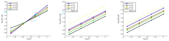
Figure 1. The convergence orders of Example 1.

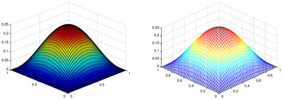
Figure 2. The exact solution u (left) and numerical solution $u_h$ (right) at $t=0.5$. Example 1.

Example 2.

The data are as follows:

$$\begin{array}{cc}\hfill & u(x,t)=\left(E_{\alpha }(-t^{\alpha })+t^3\right)sin(\pi x_1)sin(\pi x_2),\varphi (u(x,t))=u^3(x,t),\hfill \\ \hfill & \mathit{p}(x,t)=\left(\begin{array}{c}\pi \left(E_{\alpha }(-t^{\alpha })+t^3\right)\mathit{cos}(\pi x_1)\mathit{sin}(\pi x_2)\hfill \\ \pi \left(E_{\alpha }(-t^{\alpha })+t^3\right)\mathit{sin}(\pi x_1)\mathit{cos}(\pi x_2)\hfill \end{array}\right),\hfill \\ \hfill & f(x,t)=D_t^{\alpha }u(x,t)-div(\mathit{p}(x,t))+\varphi (u(x,t)),\hfill \end{array}$$

where $E_{\alpha }(z)={\displaystyle \sum _{i=0}^{\infty }}{z}^i/\Gamma (i\alpha +1)$ is the Mittag-Leffler function. The solution $u(x,t)$ displays typical layer behavior near $t=0$.

Errors $\left|\right||u-u_h\left|\right||$, $\left|\right||\nabla (u-u_h)|\left|\right|$ and $\left|\right||\mathit{p}-{\mathit{p}}_h\left|\right||$ are shown in Table 2. The relationships between ${log}_{10}(error)$ and ${log}_{10}(node)$ of $\left|\right||u-u_h\left|\right||$, $\left|\right||\nabla \left(u-u_h\right)\left|\right||$ and $\left|\right||\mathit{p}-{\mathit{p}}_h\left|\right||$ are show in Figure 3. The numerical results and convergent rates are consistent with our theoretical results. In Figure 4, we show the profiles of the exact solution u and the numerical solution $u_h$ with $\alpha =0.6$, $N=40$, $h=1/40$ and $t=0.5$.

Table 2. Errors $\left|\right||u-u_h\left|\right||$, $\left|\right||\mathit{p}-{\mathit{p}}_h\left|\right||$ and $\left|\right||\nabla \left(u-u_h\right)\left|\right||$ for different $\alpha$, Example 2.

$\mathit{\alpha }$	N	10	20	40	80
	$\mathbf{h}$	$\mathbf{1}/\mathbf{10}$	$\mathbf{1}/\mathbf{20}$	$\mathbf{1}/\mathbf{40}$	$\mathbf{1}/\mathbf{80}$
	$\left|\right||u-u_h\left|\right||$	$8.36251\times {10}^{-2}$	$2.40198\times {10}^{-2}$	$6.82853\times {10}^{-3}$	$1.94998\times {10}^{-3}$
0.2	$\left|\right||\nabla \left(u-u_h\right)\left|\right||$	$6.45852\times {10}^{-2}$	$3.23041\times {10}^{-2}$	$1.61823\times {10}^{-2}$	$8.07615\times {10}^{-3}$
	$\left|\right||\mathit{p}-{\mathit{p}}_h\left|\right||$	$6.85127\times {10}^{-2}$	$3.42632\times {10}^{-2}$	$1.71315\times {10}^{-2}$	$8.56524\times {10}^{-3}$
	$\left|\right||u-u_h\left|\right||$	$7.42563\times {10}^{-2}$	$2.43186\times {10}^{-2}$	$7.96018\times {10}^{-3}$	$2.58369\times {10}^{-3}$
0.4	$\left|\right||\nabla \left(u-u_h\right)\left|\right||$	$5.85276\times {10}^{-2}$	$2.93641\times {10}^{-2}$	$1.46403\times {10}^{-2}$	$7.32116\times {10}^{-3}$
	$\left|\right||\mathit{p}-{\mathit{p}}_h\left|\right||$	$6.25463\times {10}^{-2}$	$3.12746\times {10}^{-2}$	$1.56407\times {10}^{-2}$	$7.82533\times {10}^{-3}$
	$\left|\right||u-u_h\left|\right||$	$5.86504\times {10}^{-2}$	$2.21237\times {10}^{-2}$	$8.41062\times {10}^{-3}$	$3.20240\times {10}^{-3}$
0.6	$\left|\right||\nabla \left(u-u_h\right)\left|\right||$	$4.63425\times {10}^{-2}$	$2.32720\times {10}^{-2}$	$1.16814\times {10}^{-2}$	$5.89105\times {10}^{-3}$
	$\left|\right||\mathit{p}-{\mathit{p}}_h\left|\right||$	$5.42638\times {10}^{-2}$	$2.72328\times {10}^{-2}$	$1.37642\times {10}^{-2}$	$6.96223\times {10}^{-3}$
	$\left|\right||u-u_h\left|\right||$	$4.96425\times {10}^{-2}$	$2.16054\times {10}^{-2}$	$9.30749\times {10}^{-3}$	$3.99852\times {10}^{-3}$
0.8	$\left|\right||\nabla \left(u-u_h\right)\left|\right||$	$3.84265\times {10}^{-2}$	$1.92145\times {10}^{-2}$	$9.62712\times {10}^{-3}$	$4.83315\times {10}^{-3}$
	$\left|\right||\mathit{p}-{\mathit{p}}_h\left|\right||$	$4.51456\times {10}^{-2}$	$2.26731\times {10}^{-2}$	$1.14805\times {10}^{-2}$	$5.74137\times {10}^{-3}$

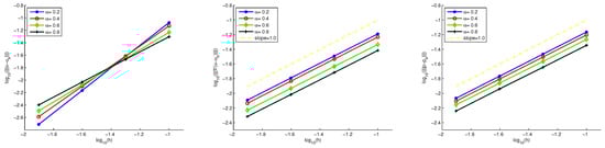
Figure 3. The convergence orders of Example 2.

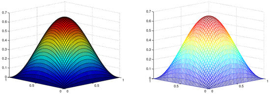
Figure 4. The exact solution u (left) and numerical solution $u_h$ (right) at $t=0.5$. Example 2.

6. Discussion

In this paper, an ICPMFE for STFDEs was investigated. Compared to classic MFEM, it can significantly improve computational efficiency. We derived the unconditional stability and convergence results $∥u^n-u_h^n∥=\mathcal{O}\left(h^{k+1}+N^{-min\{2-\alpha ,r(1+\alpha )\}}\right)$, $∥{\mathit{p}}^n-{\mathit{p}}_h^n∥=\mathcal{O}\left(h^k+N^{-min\{2-\alpha ,r(1+\alpha )\}}\right)$, $∥\nabla \left(u^n-u_h^n\right)∥=\mathcal{O}\left(h^k+N^{-min\{2-\alpha ,r(1+\alpha )\}}\right)$. In future work, we can use a two-grid method and a fast algorithm based on the sum-of-exponential technique combined with FEM or MFEM to solve this problem.

References

- Podlubny, I. Fractional Differential Equations; Academic Press: San Diego, CA, USA, 1999. [Google Scholar]
- Li, C.; Chen, A. Numerical methods for fractional partial differential equations. Int. J. Comput. Math. 2018, 95, 1048–1099. [Google Scholar] [CrossRef]
- Li, C.; Zeng, F. Numerical Methods for Fractional Calculas; Chapman and Hall/CRC Press: Boca Raton, FL, USA, 2015. [Google Scholar]
- Liu, F.; Zhuang, P.; Liu, Q. Numerical Methods for Fractional Partial Differential Equations and Their Applications; Science Press: Beijing, China, 2015. [Google Scholar]
- Li, X.; Xu, C. A space-time spectral method for the time fractional diffusion equation. SIAM J. Numer. Anal. 2009, 47, 2108–2131. [Google Scholar] [CrossRef]
- Lin, Y.; Xu, C. Finite difference/spectral approximation for the time-fractional diffusion equation. J. Comput. Phys. 2007, 225, 1533–1552. [Google Scholar] [CrossRef]
- Stynes, M.; O’Riordan, E.; Gracia, J. Error analysis of a finite difference method on graded meshes for a time-fractional diffusion equation. SIAM J. Numer. Anal. 2017, 55, 1057–1079. [Google Scholar] [CrossRef]
- Jin, B.; Lazarov, R.; Pasciak, J.; Zhou, Z. Error analysis of semidiscrete finite element methods for inhomogeneous time-fractional diffusion. IMA J. Numer. Anal. 2015, 35, 561–582. [Google Scholar] [CrossRef]
- Nochetto, R.; Otárola, E.; Salgado, A. A PDE approach to space-time fractional parabolic problems. SIAM J. Numer. Anal. 2016, 54, 848–873. [Google Scholar] [CrossRef]
- Feng, R.; Liu, Y.; Hou, Y.; Li, H.; Fang, Z. Mixed element algorithm based on a second-order time approximation scheme for a two-dimensional nonlinear time fractional coupled sub-diffusion model. Eng. Comput. 2022, 38, 51–68. [Google Scholar] [CrossRef]
- Shi, Z.; Zhao, Y.; Liu, F.; Tang, Y.; Wang, F.; Shi, Y. High accuracy analysis of an H1-Galerkin mixed finite element method for two-dimensional time fractional diffusion equations. Comput. Math. Appl. 2017, 74, 1903–1914. [Google Scholar] [CrossRef]
- Li, B.; Luo, H.; Xie, X. A space-time finite element method for fractional wave problems. Numer. Algor. 2020, 85, 1095–1121. [Google Scholar] [CrossRef]
- Li, B.; Wang, T.; Xie, X. Numerical analysis of two Galerkin discretizations with graded temporal grids for fractional evolution equations. J. Sci. Comput. 2020, 85, 59. [Google Scholar] [CrossRef]
- Liu, F.; Zhuang, P.; Turner, I.; Burrage, K.; Anh, V. A new fractional finite volume method for solving the fractional diffusion equation. Appl. Math. Model. 2014, 38, 3871–3878. [Google Scholar] [CrossRef]
- Li, M.; Zhao, J.; Huang, C.; Chen, S. Nonconforming virtual element method for the time fractional reaction-subdiffusion equation with non-smooth data. J. Sci. Comput. 2019, 81, 1823–1859. [Google Scholar] [CrossRef]
- Gu, X.; Sun, H.; Zhang, Y.; Zhao, Y. Fast implicit difference schemes for time-space fractional diffusion equations with the integral fractional Laplacian. Math. Methods Appl. Sci. 2021, 44, 441–463. [Google Scholar] [CrossRef]
- Jiang, S.; Zhang, J.; Zhang, Q.; Zhang, Z. Fast evaluation of the Caputo fractional derivative and its applications to fractional diffusion equations. Commun. Comput. Phys. 2017, 21, 650–678. [Google Scholar] [CrossRef]
- Shen, J.; Sun, Z.; Du, R. Fast finite difference schemes for time-fractional diffusion equations with a weak singularity at initial time. East Asian J. Appl. Math. 2018, 8, 834–858. [Google Scholar] [CrossRef]
- Alikhanov, A.; Huang, C. A high-order L2 type difference scheme for the time-fractional diffusion equation. Appl. Meth. Comput. 2021, 411, 126545. [Google Scholar] [CrossRef]
- Ren, J.; Liao, H.; Zhang, J.; Zhang, Z. Sharp H1-norm error estimates of two time-stepping schemes for reaction-subdiffusion problems. J. Comput. Appl. Math. 2021, 389, 113352. [Google Scholar] [CrossRef]
- Li, D.; Wu, C.; Zhang, Z. Linearized Galerkin fems for nonlinear time fractional parabolic problems with non-smooth solutions in time direction. J. Sci. Comput. 2019, 80, 403–419. [Google Scholar] [CrossRef]
- Zhao, Y.; Gu, X.; Ostermann, A. A preconditioning technique for an all-at-once system from Volterra subdiffusion equations with graded time steps. J. Sci. Comput. 2021, 88, 11. [Google Scholar] [CrossRef]
- Afolabi, Y.; Biala, T.; Iyiola, O.; Khaliq, A.; Wade, B. A second-order Crank-Nicolson-type scheme for nonlinear space-time reaction-diffusion equations on time-graded meshes. Fractal Fract. 2023, 7, 40. [Google Scholar] [CrossRef]
- Qin, H.; Chen, X.; Zhou, B. A family of transformed difference schemes for nonlinear time-fractional equations. Fractal Fract. 2023, 7, 96. [Google Scholar] [CrossRef]
- Xu, J. Two-Grid discretization techniques for linear and nonlinear PDEs. SIAM J. Numer. Anal. 1996, 33, 1759–1777. [Google Scholar] [CrossRef]
- Zlámal, M. Finite element methods for nonlinear parabolic equations. RAIRO Model. Anal. Numer. 1997, 11, 93–107. [Google Scholar] [CrossRef]
- Larsson, S.; Thomée, V.; Zhang, N. Interpolation of coefficients and transformation of dependent variable in element methods for the nonlinear heat equation. Math. Meth. Appl. Sci. 1989, 11, 105–124. [Google Scholar] [CrossRef]
- Xie, Z.; Chen, C. The interpolated coefficient FEM and its application in computing the multiple solutions of semilinear elliptic problems. Int. J. Numer. Anal. Model. 2005, 2, 97–106. [Google Scholar]
- Pani, A. An H1-Galerkin mixed finite element methods for parabolic partial differential equations. SIAM J. Numer. Anal. 1998, 35, 712–727. [Google Scholar] [CrossRef]
- Yang, D. A splitting positive definite mixed element method for miscible displacement of compressible flow in porous media. Numer. Methods Partial Differ. Eq. 2001, 17, 229–249. [Google Scholar] [CrossRef]
- Chen, S.; Chen, H. New mixed element schemes for a second-order elliptic problem. Math. Numer. Sin. 2010, 32, 213–218. (In Chinese) [Google Scholar]
- Hou, T.; Jiang, W.; Yang, Y.; Leng, H. Two-grid − P1 mixed finite element methods combined with Crank-Nicolson scheme for a class of nonlinear parabolic equations. Appl. Numer. Math. 2019, 137, 136–150. [Google Scholar] [CrossRef]
- Li, Q.; Chen, Y.; Huang, Y.; Wang, Y. Two-grid methods for semilinear time fractional reaction diffusion equations by expanded mixed finite element method. Appl. Numer. Math. 2020, 157, 38–54. [Google Scholar] [CrossRef]
- Henry, B.; Wearne, S. Fractional reaction-diffusion. Physica A 2000, 276, 448–455. [Google Scholar] [CrossRef]
- Angstmann, C.; Henry, B. Time fractional Fisher-KPP and Fitzhugh-Nagumo equations. Entropy 2020, 22, 1035. [Google Scholar] [CrossRef]
- Brezzi, F.; Fortin, M. Mixed and Hybrid Finite Element Methods; Springer: Berlin, Germany, 1999. [Google Scholar]
- Lord, G.; Powell, C.; Shardlow, T. An Introduction to Computational Stochastic PDEs; Cambridge University Press: Cambridge, UK, 2014. [Google Scholar]
- Huang, C.; Stynes, M. Optimal spatial H1-norm analysis of a finite element method for a time-fractional diffusion equation. J. Comput. Appl. Math. 2020, 367, 112435. [Google Scholar] [CrossRef]
- Huang, C.; Stynes, M. Superconvergence of a finite element method for the multi-term time-fractional diffusion problem. J. Sci. Comput. 2020, 82, 10. [Google Scholar] [CrossRef]
- Ciarlet, P. The Finite Element Method for Elliptic Problems; North-Holland: Amsterdam, The Netherlands, 1978.
Disclaimer/Publisher’s Note: The statements, opinions and data contained in all publications are solely those of the individual author(s) and contributor(s) and not of MDPI and/or the editor(s). MDPI and/or the editor(s) disclaim responsibility for any injury to people or property resulting from any ideas, methods, instructions or products referred to in the content. |
© 2023 by the authors. Licensee MDPI, Basel, Switzerland. This article is an open access article distributed under the terms and conditions of the Creative Commons Attribution (CC BY) license (https://creativecommons.org/licenses/by/4.0/).