Article

Modeling the Transmission Dynamics of Coronavirus Using Nonstandard Finite Difference Scheme

1
Department of Mathematics, Institute of Numerical Sciences, Gomal University, Dera Ismail Khan 29050, Pakistan
2
School of Mathematics and Data Sciences, Changji University, Changji 831100, China
3
Department of Mathematics, Faculty of Science, University of Maragheh, Maragheh 83111-55181, Iran
*
Author to whom correspondence should be addressed.
Fractal Fract. 2023, 7(6), 451; https://doi.org/10.3390/fractalfract7060451
Submission received: 17 April 2023 / Revised: 28 May 2023 / Accepted: 30 May 2023 / Published: 31 May 2023

Abstract

:
A nonlinear mathematical model of COVID-19 containing asymptomatic as well as symptomatic classes of infected individuals is considered and examined in the current paper. The largest eigenvalue of the next-generation matrix known as the reproductive number is obtained for the model, and serves as an epidemic indicator. To better understand the dynamic behavior of the continuous model, the unconditionally stable nonstandard finite difference (NSFD) scheme is constructed. The aim of developing the NSFD scheme for differential equations is its dynamic reliability, which means discretizing the continuous model that retains important dynamic properties such as positivity of solutions and its convergence to equilibria of the continuous model for all finite step sizes. The Schur–Cohn criterion is used to address the local stability of disease-free and endemic equilibria for the NSFD scheme; however, global stability is determined by using Lyapunov function theory. We perform numerical simulations using various values of some key parameters to see more characteristics of the state variables and to support our theoretical findings. The numerical simulations confirm that the discrete NSFD scheme maintains all the dynamic features of the continuous model.

1. Introduction

Infectious diseases, earthquakes, destructive floods, climate change, and world wars are just a few of the many challenges and difficulties that humanity has faced throughout history. These events have a significant negative impact on people’s lives and on civilizations. Among these difficulties, infectious diseases are major problem for humanity and have a negative impact on the economies, education, and tourism industry of many nations. The human immunodeficiency virus (HIV), hepatitis B virus (HBV), Ebola, Lassa fever, cholera, influenza, malaria, smallpox, and most recently COVID-19 are deadly diseases that have plagued human life [1,2,3]. In December 2019, the Chinese city of Wuhan announced the first case of a new COVID-19, which is exceedingly hazardous and contagious [4]. The virus immediately spread around the world. COVID-19 [5,6,7] has spread swiftly around the globe, since it has been shown to have a greater heightened level of infection and to be a greater pandemic danger than SARS. The WHO classified the COVID-19 outbreak as a worldwide pandemic on March 11, due to the sudden increase in transmission. Some of the symptoms of COVID-19 include fever, cough, congestion, tiredness, vomiting, headache, diarrhea, dyspnea, and lymphopenia [8]. The incubation period for COVID-19 persists for 5 days on average, although it can last up to 14 days [9].
Researchers are employing fractional- and integer-order mathematical models to describe various physical phenomena [10,11,12,13,14,15]. Numerous researchers have developed a wide variety of mathematical models to assess the dynamic behavior and transmission of COVID-19 [16,17,18,19,20]. By using a mathematical model, we can focus on how an infectious disease spreads throughout a population. These models may be utilized to enhance all of their sources and to more successfully carry out control operations [21,22,23]. The authors in [24] investigated the COVID-19 mathematical model combined with the resistive compartment and quarantine class. The model is completely different from the previous models that have been described in the literature, due to the quarantine and resistive classes. Peter et al. [25] evaluated the COVID-19 disease model by focusing on real data that evaluate the effect of various management techniques on the transmission of COVID-19 in a human population. Researchers [26,27,28] have extensively studied the novel COVID-19 through mathematical models from various perspectives. They focused on local and global dynamics, numerical methods, and stability theory.
Recently, Sabir et al. [29] studied and analyzed a COVID-9 mathematical model by focusing on the genuine information that appraises the contact of some administration techniques on the transmission of COVID-19 in a human populace. The authors employed a scaled conjugate gradient neural networks (SCGNNs) procedure to examine the numerical presentation of a nonlinear COVID-19 mathematical model. In order to analyze biological sustainability as well as various aspects of the model, the discrete NSFD scheme is developed for the continuous model. At present, the primary concern of the qualitative theory of differential equations is to deal with persistent objects, i.e., equilibrium points and their dynamic features such as stability and instability, as well as other global aspects such as domain invariance and variational structures. As a result, the notion of developing numerical schemes does not focus on approximation issues, but instead deals with certain dynamic information arising, leading to dynamic numerical schemes. The idea of an NSFD scheme was, in fact, commenced by Mickens [30]. He used the term NSFD scheme to distinguish the new numerical scheme from the old SFD (standard finite difference) schemes. The SFD schemes cannot precisely retain the basic dynamic aspects of the differential models, resulting in numerical solutions that differ from the solutions of the original systems. On the other hand, the NSFD scheme is introduced to compensate for the weaknesses of the SFD schemes. The positivity and boundedness properties of solutions are performed to better comprehend the dynamics of the model. The local and global stability of disease-free and endemic equilibria is discussed for the NSFD scheme by using a variety of theories and criteria. The results demonstrate that the aforementioned scheme is unconditionally stable and suitable for the continuous model, which produces incredibly accurate and efficient results.
The following is the layout of the paper: in Section 2, the mathematical model for the COVID-19 epidemic disease is presented. The equilibria of the model and the most important basic reproduction number are explained in Section 3. In Section 4, the discrete NSFD scheme is constructed and some basic properties, such as positivity and boundedness, are explored in Section 4.1. Our results demonstrate that the NSFD scheme is an efficient and potent method that clearly depicts the continuous model. In Section 4.2, the local stability of both the equilibria is evaluated by using Schur–Cohn criterion; however the theory of the Lyapunov function is utilized to discuss global stability in Section 4.3. Numerical simulations are performed which confirm our theoretical results. To summarize the whole manuscript, a Conclusion section is provided at the end.

2. Mathematical Model

The COVID-19 dynamic system [29], including six differential equations, is provided as follows:
d S d t = 𝜕 p + δ S β S E d E d t = β S E θ + δ + u + ϱ E d Q d t = p S + θ E φ + υ + δ Q d A d t = ϱ E + φ Q δ + r 1 A d D d t = u E + υ Q ω + δ + r 2 D d R d t = r 1 A + r 2 D δ R .
Six classes are used to categories the entire population N t , i.e., susceptible   S t , exposed E t , asymptotically diseased persons A t , symptomatic diseased persons D t , quarantined Q t and recovered R t , where N t = S t + E t + Q t + A t + D t + R t .
Model (1) is given in the following Table 1.
Figure 1 is the flow chart for mathematical Model (1) which consists of the six aforementioned categories, S t , E t , A t , D t , Q t , and R t .
We assume that all of the parameters in Model (1) attain positive constant values. As the first five equations of Model (1) are independent of   R t , therefore, for the upcoming calculation, our focus of discussion will be the following reduced model.
d S d t = 𝜕 p + δ S β S E d E d t = β S E θ + δ + u + ϱ E d Q d t = p S + θ E φ + υ + δ Q d A d t = ϱ E + φ Q δ + r 1 A d D d t = u E + υ Q ω + δ + r 2 D

3. Equilibria and Basic Reproduction Number ( R 0 )

3.1. Equilibria of Model

The disease-free equilibrium (DFE) point is attained by equating the right side of Model (2) to zero. If we represent DFE by E 0 = S 0 , E 0 , Q 0 ,   A 0 , D 0 for Model (2), then it is simple to determine DFE as E 0 = 𝜕 p + δ , 0 , 0 , 0 , 0 . The proposed Model (2) is simultaneously solved for the state variables S , E , Q , A , and D to find the disease endemic equilibrium (DEE) point. If the DEE point is represented by E * S * , E * , Q * , A * , D * , then model (2) yields S * = β S * E * 𝜕 p + δ , E * = β S * E * θ + δ + u + ϱ , Q * = p S * + θ E * φ + υ + δ , A * = ϱ E * + ϕ Q * δ + r 1 , and D * = u E * + υ Q * ω + δ + r 2 .

3.2. Basic Reproduction Number ( R 0 )

The spread of the disease, the size of the population, and the length of the sickness period all have a direct impact on the transmissibility of secondary infections. Although a precise estimate of secondary infections cannot be given, epidemiological studies can yield an approximate estimate, known as the basic reproduction number [31]. To calculate R 0 , we utilize the translation V x and transmission F x matrices, respectively. Let x = E , Q ,   A ,   D , then for System (2) these can be represented as
F x = β S E 0 0 0 ,   and   V x = θ + δ + u + ϱ E p S θ E + φ + υ + δ Q ϱ E ϕ Q + δ + r 1 A u E υ Q + ω + δ + r 2 D .
As R 0 = ρ F V 1 , therefore, the simple calculation employs
R 0 = 𝜕 β p + δ θ + δ + u + ϱ

4. The NSFD Scheme

The NSFD scheme is used to provide a broad way of creating discrete models and finding the numerical solution of ordinary as well as partial differential equations. According to Shokri et al. [32], the investigation of the NSFD scheme depends on two factors. First, how to approximate nonlinear terms in the most appropriate way, and second, how to discretized the derivative. Usually, the first order derivative d f d x is written as f x + h f x h , where h stands for step size. According to Mickens [33,34], this term can be written as f x + h f x φ h , where φ h is an increasing function known as the denominator function. In order to better comprehend the dynamics of the COVID-19 disease, we will focus on the simplest denominator function φ h = h in the current work, rather than the general denominator functions that can be seen in [33,34].
The numerical estimates of S t , E t , Q t , A t   and   D t at t = n h for model (2) are denoted as S n ,   E n , Q n ,   A n , D n , where n is a nonnegative integer and h specifies the time step size, which should also be nonnegative [35]. Model (2) afterwards enables us to write
S n + 1 S n h = 𝜕 p + δ S n + 1 β S n + 1 E n E n + 1 E n h = β S n + 1 E n θ + δ + u + ϱ E n + 1 Q n + 1 Q n h = p S n + 1 + θ E n + 1 φ + υ + δ Q n + 1 A n + 1 I A n h = ϱ E n + 1 + ϕ Q n + 1 δ + r 1 A n + 1 D n + 1 D n h = u E n + 1 + υ Q n + 1 ω + δ + r 2 D n + 1
After simplification, the explicit form of the NSFD scheme (3) becomes
S n + 1 = h 𝜕 + S n 1 + h p + δ + β E n E n + 1 = E n + h β S n + 1 E n 1 + h θ + δ + u + ϱ Q n + 1 = h p S n + 1 + θ E n + 1 + Q n 1 + h φ + υ + δ A n + 1 = h ϱ E n + 1 + φ Q n + 1 + A n 1 + h δ + r 1 D n + 1 = h u E n + 1 + υ Q n + 1 + D n 1 + h ω + δ + r 2

4.1. Positivity and Boundedness of NSFD Scheme

We assume that the initial values of discrete scheme (4) are nonnegative, i.e., S 0 0 , E 0 0 , Q 0 0 , A 0 0 , D 0 0 . These variables have estimated quantities which are also nonnegative, due to the assumptions S n 0 ,   E n 0 , Q n 0 , A n 0 , D n 0 . Therefore, the solutions of the NSFD scheme (4) imply the positivity of scheme (4), i.e., S n + 1 0 , E n + 1 0 , Q n + 1 0 , A n + 1 0 , D n + 1 0 . In order to discuss the boundedness of the solutions of the NSFD system (4), we consider T n = S n + E n + Q n + A n + D n . Then
T n + 1 T n h = 𝜕 p + δ T n + 1
i.e.,
  ( 1 + p + δ ) T n + 1 = h 𝜕 + T n
Therefore, we obtain
T n + 1 h 𝜕 1 + h p + δ + T n 1 + h p + δ h k + 1 n 1 ( 1 + h p + δ k + T 0 1 ( 1 + h p + δ n
If 0 < T 0 < 𝜕 p + δ , then by employing Gronwall’s inequality, we obtain
T n 𝜕 p + q 1 1 1 + h p + δ n + T 0 1 ( 1 + h p + δ n = 𝜕 p + δ + T 0 𝜕 p + δ 1 ( 1 + h p + δ n
Since 1 ( 1 + h p + δ n < 1 , so we obtain T n 𝜕 p + δ as n . This shows that the solutions of the system (4) are bounded, and the feasible region becomes
B = S n + E n + Q n + A n + D n : 0 S n + E n + Q n + A n + D n 𝜕 p + δ
In order to verify the local stability of both equilibria for the NSFD scheme (4), we consider
S n + 1 = h 𝜕 + S n 1 + h p + δ + β E n = g 1 E n + 1 = E n + h β S n + 1 E n 1 + h θ + δ + u + ϱ = g 2 Q n + 1 = h p S n + 1 + θ E n + 1 + Q n 1 + h φ + υ + δ = g 3 A n + 1 = h ϱ E n + 1 + φ Q n + 1 + A n 1 + h δ + r 1 = g 4 D n + 1 = h u E n + 1 + υ Q n + 1 + D n 1 + h ω + δ + r 2 = g 5

4.2. Local Stability of Equilibria

To prove that the DFE point is locally asymptotically stable, we will use the Schur–Cohn criterion [36,37], stated in the following Lemma 1.
Lemma 1. 
The roots of Γ 2 B Γ + C = 0 guarantee Γ j < 1   f o r   j = 1 , 2 , if and only if the requirements given in the following are fulfilled.
  • C < 1 ,
  • 1 + B + C > 0 ,
  • 1 B + C > 0 , where B denotes trace and C indicates determinant of the Jacobian matrix.
Theorem 1. 
For all h > 0 , the DFE point is locally asymptotically stable for the NSFD Model (4) whenever R 0 < 1 .
Proof. 
Based on the information provided above, the Jacobian matrix can be expressed as
J S , E , Q , A , D = 𝜕 g 1 𝜕 S 𝜕 g 1 𝜕 E 𝜕 g 1 𝜕 Q 𝜕 g 1 𝜕 A 𝜕 g 1 𝜕 D 𝜕 g 2 𝜕 S 𝜕 g 2 𝜕 E 𝜕 g 2 𝜕 Q 𝜕 g 2 𝜕 A 𝜕 g 2 𝜕 D 𝜕 g 3 𝜕 S 𝜕 g 3 𝜕 E 𝜕 g 3 𝜕 Q 𝜕 g 3 𝜕 A 𝜕 g 3 𝜕 D 𝜕 g 4 𝜕 S 𝜕 g 4 𝜕 E 𝜕 g 4 𝜕 Q 𝜕 g 4 𝜕 A 𝜕 g 4 𝜕 D 𝜕 g 5 𝜕 S 𝜕 g 5 𝜕 E 𝜕 g 5 𝜕 Q 𝜕 g 5 𝜕 A 𝜕 g 5 𝜕 D
where g 1 , g 2 , g 3 , g 4   and g 5 are provided in (5). We first perceive all the derivatives used in (6) as follows:
g 1 S = 1 1 + h p + δ + β E n , g 1 E = h 1 + h p + δ + β E n 2 , g 1 A = 0 , g 1 D = 0 ,   g 1 Q = 0 , g 2 S = 0 , g 2 E = 1 + h β S n + 1 1 + h θ + δ + u + ϱ , g 1 A = 0 , g 2 D = 0 ,   g 2 Q = 0 , g 3 S = h p 1 + h φ + υ + δ , g 3 E = h θ 1 + h φ + υ + δ , g 3 Q = 1 1 + h φ + υ + δ , g 3 A = 0 ,   g 3 D = 0 , g 4 S = 0 , g 4 E = h ϱ 1 + h δ + r 1 ,   g 4 Q = h ϕ 1 + h δ + r 1 ,   g 4 A = 1 + h ϱ 1 + h δ + r 1 , g 4 D = 0 , g 5 S = 0 ,   g 5 E = h υ 1 + h ω + δ + r 2 ,     g 5 Q = h φ 1 + h ω + δ + r 2 ,   g 5 A = 0 ,   g 5 D = 1 1 + h ω + δ + r 2 .  
Putting all the above derivatives in (6), we obtain
J = 1 1 + h p + δ + β E n h 𝜕 1 + h p + δ + β E n 2 0 0 0 0 1 + h β S n + 1 1 + h θ + δ + u + ϱ 0 0 0 h p 1 + h φ + υ + δ h θ 1 + h φ + υ + δ 1 1 + h φ + υ + δ 0 0 0 h ϱ 1 + h δ + r 1 h ϕ 1 + h δ + r 1 1 + h ϱ 1 + h δ + r 1 0 0 h υ 1 + h ω + δ + r 2 h φ 1 + h ω + δ + r 2 0 1 1 + h ω + δ + r 2
At DFE point E 0 = 𝜕 p + δ , 0 , 0 , 0 , 0 , the matrix (7) becomes
J E 0 = 1 1 + h p + δ h 𝜕 1 + h p + δ 2 0 0 0 0 1 + h β 𝜕 p + δ 1 + h θ + δ + u + ϱ 0 0 0 h p 1 + h φ + υ + δ h θ 1 + h φ + υ + δ 1 1 + h φ + υ + δ 0 0 0 h ϱ 1 + h δ + r 1 h ϕ 1 + h δ + r 1 1 + h ϱ 1 + h δ + r 1 0 0 h υ 1 + h ω + δ + r 2 h φ 1 + h ω + δ + r 2 0 1 1 + h ω + δ + r 2
In order to explain the eigenvalues, we assume
J E 0 Γ I = 0
i.e.,
1 1 + h p + δ Γ h 𝜕 1 + h p + δ 2 0 0 0 0 1 + h β 𝜕 p + δ 1 + h θ + δ + u + ϱ Γ 0 0 0 h p 1 + h φ + υ + δ h θ 1 + h φ + υ + δ 1 1 + h φ + υ + δ Γ 0 0 0 h ϱ 1 + h δ + r 1 h ϕ 1 + h δ + r 1 1 + h ϱ 1 + h δ + r 1 Γ 0 0 h υ 1 + h ω + δ + r 2 h φ 1 + h ω + δ + r 2 0 1 1 + h ω + δ + r 2 Γ = 0
After simple calculations, (8) yields
Γ 1 1 1 + h ω + δ + r 2 Γ 2 1 + h ϱ 1 + h δ + r 1 Γ 3 1 1 + h φ + υ + δ 1 1 + h p + δ Γ h 𝜕 1 + h p + δ 2 0 1 + h β 𝜕 p + δ 1 + h θ + δ + u + ϱ Γ = 0
The Equation (9) provides Γ 1 = 1 1 + h ω + δ + r 2 < 1 , Γ 2 = 1 + h ϱ 1 + h δ + r 1 < 1 and Γ 3 = 1 1 + h φ + υ + δ < 1 . To find other eigenvalues, we take
1 1 + h p + δ Γ h 𝜕 1 + h p + δ 2 0 1 + h β 𝜕 p + δ 1 + h θ + δ + u + ϱ Γ = 0
i.e.,
Γ 2 Γ 1 1 + h p + δ + 1 + 𝜕 h β p + δ 1 + h θ + δ + u + ϱ + 1 + 𝜕 h β p + δ 1 + h p + δ 1 + h θ + δ + u + ϱ = 0
Comparing Equation (10) with Γ 2 B Γ + C = 0 , we obtain B = 1 1 + h p + δ + 1 + 𝜕 h β p + δ 1 + h θ + δ + u + ϱ and C = 1 + 𝜕 h β p + δ 1 + h p + δ 1 + h θ + δ + u + ϱ . If R 0 < 1 ,   i.e., 𝜕 β < p + δ θ + δ + u + ϱ .
  • C = 1 + h β 𝜕 p + δ 1 + h p + δ 1 + h θ + δ + u + ϱ < 1 .
  • 1 + B + C = 1 + 1 1 + h p + δ + 1 + 𝜕 h β p + δ 1 + h θ + δ + u + ϱ + 1 + 𝜕 h β p + δ 1 + h p + δ 1 + h θ + δ + u + ϱ > 0 .
  • 1 B + C = 1 1 1 + h p + δ 1 + 𝜕 h β p + δ 1 + h θ + δ + u + ϱ + 1 + 𝜕 h β p + δ 1 + h p + δ 1 + h θ + δ + u + ϱ > 0 .
As a result, whenever R 0 < 1 , all of the requirements of the Schur–Cohn criterion mentioned in Lemma 1 are satisfied. Therefore, provided that R 0 < 1 , the DFE point E 0 of the discrete NSFD scheme (4) is locally asymptotically stable. □
Theorem 2. 
For all cases of h > 0 , the DEE point is locally asymptotically stable for the NSFD model (4) whenever R 0 > 1 .
Proof. 
We derive the Jacobian matrix similarly to Theorem 1, as follows:
J = 1 1 + h p + δ + β E n h 𝜕 1 + h p + δ + β E n 2 0 0 0 0 1 + h β S n + 1 1 + h θ + δ + u + ϱ 0 0 0 h p 1 + h φ + υ + δ h θ 1 + h φ + υ + δ 1 1 + h φ + υ + δ 0 0 0 h ϱ 1 + h δ + r 1 h ϕ 1 + h δ + r 1 1 + h ϱ 1 + h δ + r 1 0 0 h υ 1 + h ω + δ + r 2 h φ 1 + h ω + δ + r 2 0 1 1 + h ω + δ + r 2
By including DEE point E * , Equation (11) becomes
J E * = 1 1 + h p + δ + β E n * h 𝜕 1 + h p + δ + β E n * 2 0 0 0 0 1 + h β S n + 1 * 1 + h θ + δ + u + ϱ 0 0 0 h p 1 + h φ + υ + δ h θ 1 + h φ + υ + δ 1 1 + h φ + υ + δ 0 0 0 h ϱ 1 + h δ + r 1 h ϕ 1 + h δ + r 1 1 + h ϱ 1 + h δ + r 1 0 0 h υ 1 + h ω + δ + r 2 h φ 1 + h ω + δ + r 2 0 1 1 + h ω + δ + r 2
To discuss the eigenvalues, we take
J E * Γ I = 0 ,
i.e.,
1 1 + h p + δ + β E n * Γ h 𝜕 1 + h p + δ + β E n * 2 0 0 0 0 1 + h β S n + 1 * 1 + h θ + δ + u + ϱ Γ 0 0 0 h p 1 + h φ + υ + δ h θ 1 + h φ + υ + δ 1 1 + h φ + υ + δ Γ 0 0 0 h ϱ 1 + h δ + r 1 h ϕ 1 + h δ + r 1 1 + h ϱ 1 + h δ + r 1 Γ 0 0 h υ 1 + h ω + δ + r 2 h φ 1 + h ω + δ + r 2 0 1 1 + h ω + δ + r 2 Γ = 0
After simplification, (12) yields
1 1 + h ω + δ + r 2 Γ 1 + h ϱ 1 + h δ + r 1 Γ 1 1 + h φ + υ + δ Γ 1 1 + h p + δ Γ h 𝜕 1 + h p + δ 2 0 1 + h γ β S * E * 𝜕 p + δ 1 + h θ + δ + u + ϱ Γ = 0
The three roots of the Equation (13) are Γ 1 = 1 1 + h ω + δ + r 2 < 1 , Γ 2 = 1 + h ϱ 1 + h δ + r 1 < 1 and Γ 3 = 1 1 + h φ + υ + δ < 1 . To discuss other eigenvalues, we take
1 1 + h p + δ Γ h 𝜕 1 + h p + δ 2 0 1 + h γ β S * E * 𝜕 p + δ 1 + h θ + δ + u + ϱ Γ = 0
i.e.,
Γ 2 Γ 1 1 + h p + δ + 1 + h β γ S * E * 𝜕 p + δ 1 + h θ + δ + u + ϱ + 1 + h β β S * E * 𝜕 p + δ 1 + h p + δ 1 + h θ + δ + u + ϱ = 0
Comparing (14) with (10), we obtain B = 1 1 + h p + δ + 1 + h β β S * E * 𝜕 p + δ 1 + h θ + δ + u + ϱ and C = 1 + h β β S * E * 𝜕 p + δ 1 + h p + δ 1 + h θ + δ + u + ϱ . If R 0 > 1 ,   i.e., 𝜕 β > p + δ θ + δ + u + ϱ , then
  • C = 1 + h β β S * E * 𝜕 p + δ 1 + h p + δ 1 + h θ + δ + u + ϱ < 1 .
  • 1 + B + C = 1 + 1 1 + h p + δ + 1 + h β β S * E * 𝜕 p + δ 1 + h θ + δ + u + ϱ + 1 + h β β S * E * 𝜕 p + δ 1 + h p + δ 1 + h θ + δ + u + ϱ > 0 .
  • 1 B + C = 1 1 1 + h p + δ 1 + h β β S * E * 𝜕 p + δ 1 + h θ + δ + u + ϱ + 1 + h β β S * E * 𝜕 p + δ 1 + h p + δ 1 + h θ + δ + u + ϱ > 0 .
As a result, whenever R 0 > 1 , all of the requirements of the Schur–Cohn criterion stated in Lemma 1 are fulfilled. Therefore, provided that R 0 > 1 , the DEE point E * of the discrete NSFD scheme (4) is locally asymptotically stable. □

4.3. Global Stability of Equilibria

To prove the global stability of the DFE and DEE points for the NSFD scheme (4), we define the function H x 0 such that H x = y ln y 1 and, consequently ln y y 1 .
Theorem 3. 
For all cases of  h > 0 , the DFE point is globally asymptotically stable for the NSFD model (4) whenever   R 0 1 .
Proof. 
Construct a discrete Lyapunov function
P n S n ,   E n , Q n , A n , D n = S 0 H S n S 0 + ϕ 1 E n + ϕ 2 Q n + ϕ 3 A n + ϕ 4 D n
where ϕ i > 0 for all i = 1 ,   2 ,   3 ,   4 . Hence, P n > 0 for all S n > 0 ,   E n > 0 ,   Q n > 0 ,   A n > 0 , and Q n > 0 . In addition, P n = 0 , if and only if, S n = S 0 , E n = E 0 ,   A n = A 0 , D n = D 0 , and Q n = Q 0 . We take
Δ P n = P n + 1 P n
i.e.,
Δ P n = S 0 F S n + 1 S 0 + ϕ 1 E n + 1 + ϕ 2 Q n + 1 + ϕ 3 A n + 1 + ϕ 4 D n + 1 S 0 F S n S 0 + ϕ 1 E n + ϕ 3 A n + ϕ 4 D n + ϕ 3 Q n = S 0 S n + 1 S 0 S n S 0 + ln S n   S n + 1 + ϕ 1 E n + 1 E n + ϕ 2 Q n + 1 Q n + ϕ 4 D n + 1 D n
Using the inequality ln y y 1 , (15) becomes
Δ P n S n + 1 S n + S 0 1 + S n   S n + 1 + 1 + E n   E n + 1 ϕ 1 E n + 1 E n + 1 + Q n   Q n + 1 ϕ 2 Q n + 1 Q n + 1 + A n A n + 1 ϕ 3 A n + 1 A n + 1 + D n D n + 1 ϕ 4 D n + 1 D n = 1 S 0 S n + 1 S n + 1 S n 1 E n   E n + 1 ϕ 1 E n + 1 E n 1 Q n   Q n + 1 ϕ 2 Q n + 1 Q n                         1 A n A n + 1 ϕ 3 A n + 1 A n 1 D n D n + 1 ϕ 4 D n + 1 D n
By utilizing system (3), (16) can be written as
Δ P n 1 S 0 S n + 1 𝜕 p + δ S n + 1 β S n + 1 E n + 1 E n   E n + 1 ϕ 1 β S n + 1 E n θ + δ + u + ϱ E n + 1 + 1 Q n   Q n + 1 ϕ 2 p S n + 1 + θ E n + 1 φ + υ + δ Q n + 1 1 A n A n + 1 ϕ 3 ϱ E n + 1 + ϕ Q n + 1 δ + r 1 A n + 1 + 1 D n D n + 1 ϕ 4 u E n + 1 + υ Q n + 1 ω + δ + r 2 D n + 1
Let ϕ i for i = 1, 2, 3, 4 be selected so that
𝜕 p + δ S n + 1 β S n + 1 E n = ϕ 1 β S n + 1 E n θ + δ + u + ϱ E n + 1 ,   ϕ 2 p S n + 1 + θ E n + 1 φ + υ + δ Q n + 1 = ϕ 3 ϱ E n + 1 + υ Q n + 1 δ + r 1 A n + 1 ,   u E n + 1 + φ Q n + 1 ω + δ + r 2 D n + 1 = ϕ 5 r 1 A n + r 2 D n δ R n + 1 .
By including the above values, from (17) we obtain
Δ P n 1 S 0 S n + 1 𝜕 p + δ S n + 1 β S n + 1 E n + 1 E n E n + 1 ϕ 1 β S n + 1 E n θ + δ + u + ϱ E n + 1 + 1 Q n Q n + 1 ϕ 2 p S n + 1 + θ E n + 1 φ + v + δ Q n + 1 + 1 A n A n + 1 ϕ 3 ϱ E n + 1 + ϕ Q n + 1 δ + r 1 A n + 1 + 1 D n D n + 1 ϕ 4 u E n + 1 + v Q n + 1 ω + δ + r 2 D n + 1 .
Simple calculations yield
Δ P n 1 S 0 S n + 1 𝜕 + ϕ 1 β S n + 1 E n 1 A n A n + 1 ϕ 1 θ + δ + u + ϱ E n + 1 + 1 E n   E n + 1   ϕ 2 p S n + 1 + ϕ 2 θ E n + 1 + ϕ 3 ϱ E n + 1 + ϕ 3 ϕ Q n + 1 + 1 Q n   Q n + 1 ϕ 3 δ + r 1 A n + 1 + ϕ 4 u E n + 1 + ϕ 4 φ Q n + 1 + 1 D n D n + 1 ϕ 4 ω + δ + r 2 D n + 1 1 S 0   S n + 1 𝜕 1 A n A n + 1 ϕ 1 θ + δ + u + ϱ + 1 E n   E n + 1   ϕ 2 p S n + 1 1 Q n   Q n + 1 ϕ 3 δ + r 1 A n + 1 + 1 D n D n + 1 ϕ 4 φ Q n + 1
As S 0 = 𝜕 p + q , this implies S 0 p + δ = 𝜕 . By substituting 𝜕 in (18), we obtain
Δ P n 1 S 0 S n + 1 S 0 p + δ p + δ S n + 1 1 A n A n + 1 ϕ 1 θ + δ + u + ϱ + 1 E n   E n + 1   ϕ 2 p S n + 1 1 Q n   Q n + 1 ϕ 3 δ + r 1 A n + 1 + 1 D n D n + 1 ϕ 4 φ Q n + 1 = p + δ S n + 1 ( S n + 1 S 0 2 1 A n A n + 1 ϕ 1 θ + δ + u + ϱ E n + ϕ 2 p p + δ θ + δ + u + ϱ 𝜕 β R 0 ϕ 3 δ + r 1 A n + 1 + ϕ 4 φ Q n + 1 )
Hence, if R 0 1 , then from Equation (19) we employ Δ P n 0 for all n 0 . Consequently, P n is a non-increasing sequence. Therefore, there exists a constant P , such that lim n P n = P ,which suggests that lim n P n + 1 P n = 0 . From system (3) and lim n Δ P n = 0 we have lim n S n = S 0 . For the case R 0 < 1 , we have lim n S n + 1 = S 0 and lim n E n = 0 ,   lim n A n = 0 . From system (3), we achieve lim n E n = 0 , lim n D = 0 and lim n Q n = 0 . For the case R 0 = 1 , we have lim n S n + 1 = S 0 . Thus, from System (3), we obtain lim n R n = 0 , lim n Q n = 0 , lim n E n = 0 , lim n A n = 0 and lim n D n = 0 . Hence, E 0 is globally asymptotically stable.
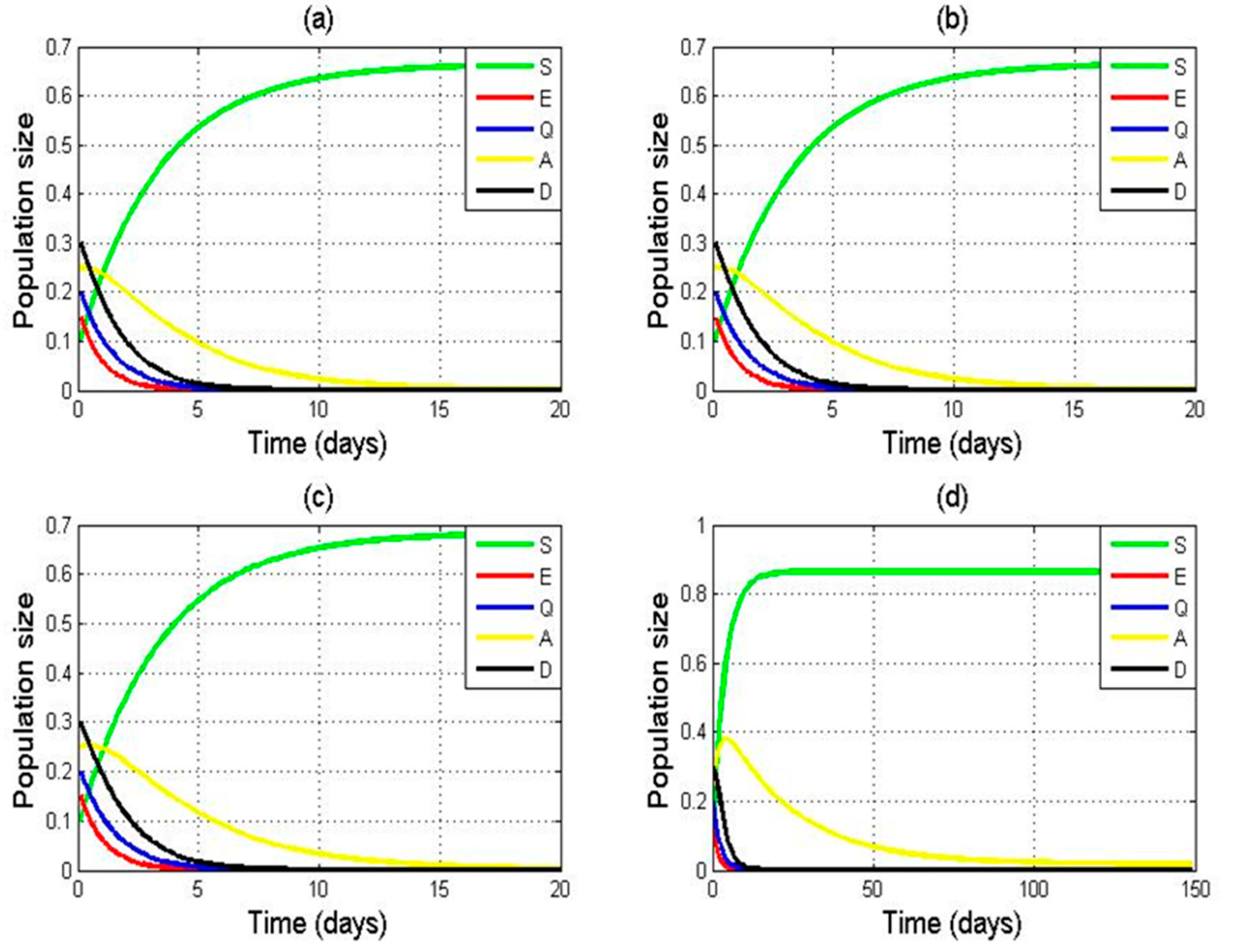
Figure 2a–d demonstrate that the solutions of the NSFD scheme (4) tend to the DFE point for any step size whenever R 0 1 . This demonstrates that the DFE point of the discrete NSFD scheme (4) is unconditionally convergent. Also, see Figure 3. □
Theorem 4. 
For all cases of h > 0 , the DEE point is globally asymptotically stable for the NSFD Model (4) whenever R 0 > 1 .
Proof. 
Let us define
V n S n ,   E n , Q n , A n , D n = S * H S n S * + ϕ 1 E * H E n E * + ϕ 2 Q * H Q n Q * + ϕ 3 A * H A n A * + ϕ 4 D * H D n D *
where ϕ i > 0 , i = 1 ,   2 ,   3 ,   4 which we will select later. It is clear that V n S n ,   E n , Q n , A n , D n > 0 for all S n > 0 ,   E n > 0 , Q n > 0 ,   A n > 0 ,   D n > 0 and V n S * , E * , Q * , A * ,   D * = 0 . Let us take
V n = V n + 1 V n ,
we obtain
V n = S * H S n + 1 S * + ϕ 1 E * H E n + 1 E * + ϕ 2 Q * H Q n + 1 Q * + ϕ 3 A * H A n + 1 A * + ϕ 4 D * H D n + 1 D *     S * H S n S * + ϕ 1 E * H E n E * + ϕ 2 Q * H Q n Q * + ϕ 3 A * H A n A * + ϕ 4 D * H D n D *
= S * S n + 1 S * S n S * + ln S n   S n + 1 + ϕ 1 E * E n + 1 E * E n E * + ln E n E n + 1 + ϕ 2 Q * Q n + 1 Q *   Q n Q * + ln Q n Q n + 1 + ϕ 3 A * A n + 1 A * A n A * + ln A n A n + 1 + ϕ 4 D * D n + 1 D * D n D * + ln D n D n + 1
By employing inequality ln y y 1 , (20) can be written as
V n S * S n + 1 S n S * + S n   S n + 1 1 + ϕ 1 E * E n + 1 E n E * + E n E n + 1 1 + ϕ 2 Q * Q n + 1 Q n Q * + Q n Q n + 1 1 +                         ϕ 3 A * A n + 1 A n A * + A n A n + 1 1 + ϕ 4 A * D n + 1 D n D * + D n D n + 1 1 = 1 S * S n + 1 S n + 1 S n + ϕ 1 1 E * E n + 1 E n + 1 E n + ϕ 2 1 Q * Q n + 1 Q n + 1   Q n + ϕ 3 1 A * A n + 1 A n + 1 A n + ϕ 4 1 D * D n + 1 D n + 1 D n
By utilizing system (3), (21) becomes
V n 1 S * S n + 1 𝜕 p + δ S n + 1 β S n + 1 E n + ϕ 1 1 E * E n + 1 β S n + 1 E n θ + δ + u + ϱ E n + 1 + ϕ 3 1 A * A n + 1 ϱ E n + 1 + ϕ Q n + 1 δ + r 1 A n + 1 + ϕ 4 1 D * D n + 1 u E n + υ Q n + 1 ω + δ + r 2 D n + 1 + ϕ 2 1 Q * Q n + 1 p S n + 1 + θ E n + 1 φ + υ + δ Q n + 1
By replacing 𝜕 = p + δ S * + γ S * E * in (22), we obtain
Δ V n 1 S * S n + 1 p + δ S * + β S * E * p + δ S n + 1 γ S n + 1 E n + ϕ 1 1 E * E n + 1 β S E                         θ + δ + υ + ϱ E * )   + ϕ 3 1 A * A n + 1 ϱ E + ϕ Q δ + r 1 A + ϕ 4 1 D * D n + 1 υ E n +                       φ Q n + 1 ω + δ + r 2 D n + 1 + ϕ 2 1 Q * Q n + 1 p S + θ E φ + υ + δ Q = 1 S * S n + 1 p + δ S * p + δ S n + 1 + ϕ 1 1 E * E n + 1 β S E θ + δ + u + ϱ E * ) + ϕ 2 1 Q * Q n + 1 p S + θ E φ + υ + δ Q + ϕ 3 1 A * A n + 1 ϱ E + ϕ Q δ +                           r 1 A + ϕ 4 1 D * D n + 1 u E n + 1 + υ Q n + 1 ω + δ + r 2 D n + 1
By substituting p + δ S * + β S * E * = ϕ 1 θ + δ + u + ϱ E * ,   θ E * = ϕ 2 δ + r 1 A * ,   ω D * = ϕ 3   ω + δ + r 2 D * in (23), we obtain
Δ V n θ S n + 1 S n + 1 S * 2 + 1 S * S n + 1 θ + δ + u + ϱ E * θ + δ + u + ϱ E * S n + 1 D n E * S * E n + 1 + ϕ 2 θ E * S n + 1 D n A * S * D * A n + 1 ϕ 1 p + δ S * + β S * E * A * E n + 1 A n + 1 E * + ϕ 2 δ + r 1 A * ϕ 3 ω D * S n + 1 D n Q * S * Q n + 1 + ϕ 3 ω D * ϕ 2 δ + r 1 A * D * D n + 1 A n + 1 D * ϕ 3 ω A * D * Q * D n + 1 = p + δ S n + 1 S n + 1 S * 2 ϕ 1 D * H S * S n + 1 + H S n + 1 D n E * S * D * E n + 1 + H A * E n + 1 A n + 1 E * + H D * A n + 1 D n + 1 A * ϕ 2 θ E * H S * S n + 1 + H S n + 1 D n D * S * D * D n + 1 + H D * D n + 1 D n + 1 A * ϕ 3 ω A * H S * S n + 1 + H S n + 1 D n Q * S * D * Q n + 1 +               H Q n + 1 D * Q * D n + 1 .
Thus, V n is a non-increasing sequence and there is a constant V , such that lim n V n = V . Therefore, lim n V n = 0 ,which implies lim n S n = S * , lim n E n = E * , lim n Q n   = Q * , lim n A n = A * ,   and   lim n D n = D * .
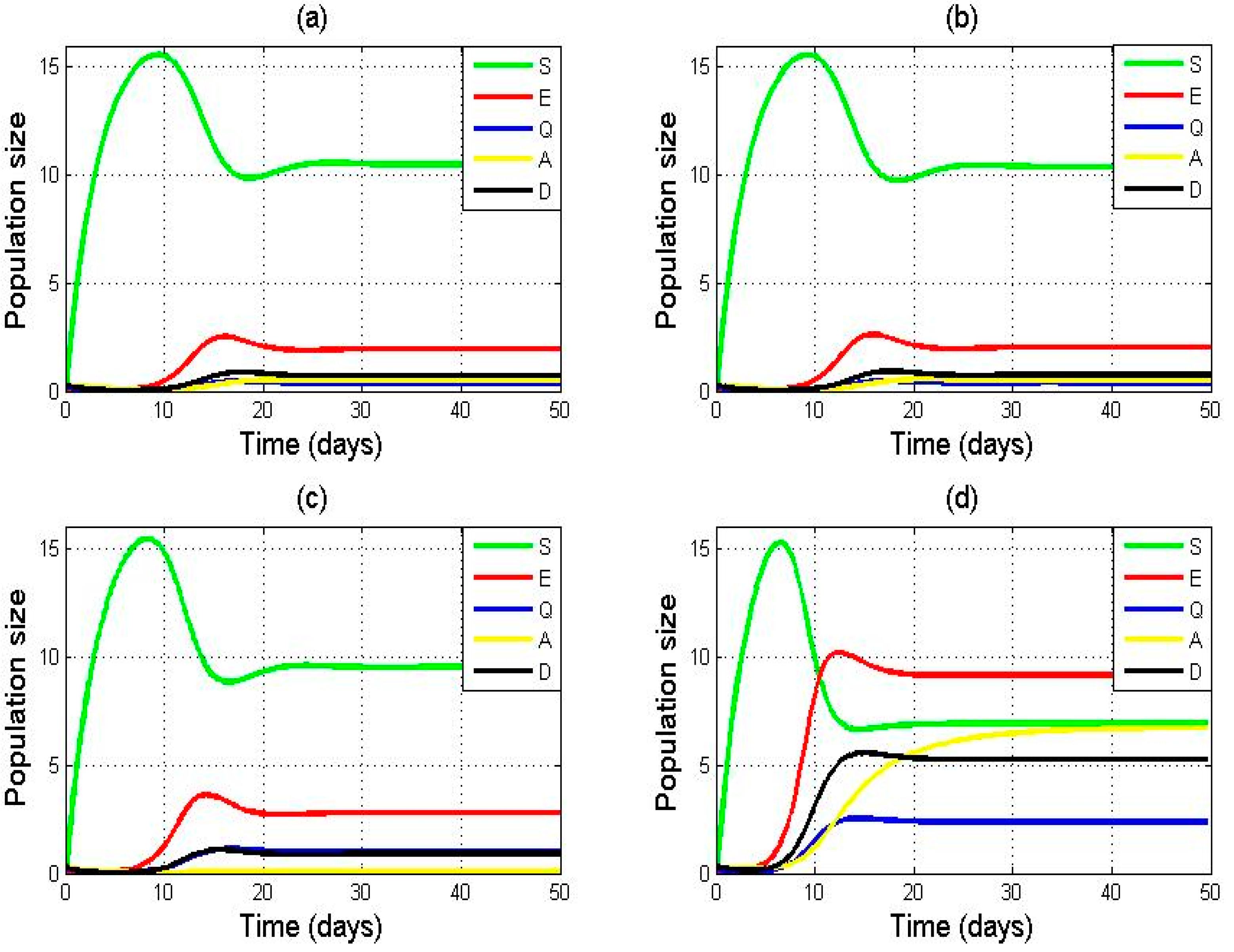
Figure 3a–d shows that whenever R 0 > 1 , the solutions of the NSFD scheme (4) tend to the DEE point for any step size. This proves the unconditional convergence of the DEE point for the discrete NSFD scheme (4) whenever R 0 > 1 .

5. Conclusions

A nonlinear mathematical model of the COVID-19 disease that includes asymptomatic as well as symptomatic classes of infected individuals is employed and analyzed in the current work. In order to properly investigate the stability of the DFE and DEE points, the critical threshold quantity   R 0 is obtained for the continuous model. The NSFD scheme is developed, which offers accurate results for all finite step sizes while maintaining key aspects of the continuous model. The boundedness and positivity of solutions for the discrete NSFD scheme are thoroughly examined. For the NSFD scheme, multiple conditions and criteria have been devised to check the local and global stability of the equilibria. It is demonstrated that the proposed discrete NSFD scheme [38,39] has the same dynamics as the continuous model, irrespective of the time step size. The outcomes present the fact that the spread of the COVID-19 epidemic disease can be effectively monitored by utilizing the NSFD scheme. The information offered in this research is useful for humanity and for the area of medicine as well. The results provided in the present paper can be used as a useful tool to forecast the emergence of the COVID-19 epidemic disease. All the aforementioned qualitative features are also verified by numerical simulations.
In our future study, we intend to investigate additional generalized epidemic models with characteristics comparable to the one under consideration in order to gain a deeper understanding of disease transmission dynamics. The dynamic behavior of the epidemic models will be investigated using the Euler, RK-4, and NSFD numerical schemes.

Author Contributions

Conceptualization, I.U.K.; methodology, I.U.K.; software, I.U.K. and A.H.; validation, S.L. and A.S.; formal analysis, A.H.; writing—original draft preparation, A.H.; writ-ing—review and editing, S.L. and A.S.; visualization, S.L.; funding acquisition, A.S. All authors have read and agreed to the published version of the manuscript.

Funding

This research received no external funding.

Data Availability Statement

Not applicable.

Acknowledgments

The authors wish to thank the anonymous referees for their careful reading of the manuscript and their fruitful comments and suggestions which improved the presentation of this paper.

Conflicts of Interest

The authors declare no conflict of interest.

References

  1. Soresina, A.; Moratto, D.; Chiarini, M.; Paolillo, C.; Baresi, G.; Focà, E.; Badolato, R. Two X-linked agammaglobulinemia patients develop pneumonia as COVID-19 manifestation but recover. Pediatr. Allergy Immunol. 2020, 31, 565–569. [Google Scholar] [CrossRef]
  2. Liu, C.; Zhou, Q.; Li, Y.; Garner, L.V.; Watkins, S.P.; Carter, L.J.; Smoot, J.; Gregg, A.C.; Daniels, A.D.; Jervey, S.; et al. Research and development on therapeutic agents and vaccines for COVID-19 and related human coronavirus diseases. ACS Cent. Sci. 2020, 6, 315–331. [Google Scholar] [CrossRef]
  3. Bootsma, M.C.; Ferguson, N.M. The effect of public health measures on the 1918 influenza pandemic in US cities. Proc. Natl. Acad. Sci. USA 2007, 104, 7588–7593. [Google Scholar] [CrossRef]
  4. Imperial College COVID-19 Response Team. Impact of Non-Pharmaceutical Interventions (NPIs) to Reduce COVID-19 Mortality and Healthcare Demand; Imperial College: London, UK, 2020. [Google Scholar]
  5. Aba Oud, M.A.; Ali, A.; Alrabaiah, H.; Ullah, S.; Khan, M.A.; Islam, S. A fractional order mathematical model for COVID-19 dynamics with quarantine, isolation, and environmental viral load. Adv. Differ. Equ. 2021, 2021, 106. [Google Scholar] [CrossRef]
  6. Mahmoudi, M.R.; Heydari, M.H.; Qasem, S.N.; Mosavi, A.; Band, S.S. Principal component analysis to study the relations between the spread rates of COVID-19 in high risks countries. Alex. Eng. J. 2021, 60, 457–464. [Google Scholar] [CrossRef]
  7. Xu, R.; Cui, B.; Duan, X.; Zhang, P.; Zhou, X.; Yuan, Q. Saliva: Potential diagnostic value and transmission of 2019-n CoV. Int. J. Oral Sci. 2020, 12, 1–6. [Google Scholar] [CrossRef]
  8. Huang, C.; Wang, Y.; Li, X.; Ren, L.; Zhao, J.; Hu, Y.; Cao, B. Clinical features of patients infected with 2019 novel coronavirus in Wuhan, China. Lancet 2020, 395, 497–506. [Google Scholar] [CrossRef]
  9. Linton, N.M.; Kobayashi, T.; Yang, Y.; Hayashi, K.; Akhmetzhanov, A.R.; Jung, S.M.; Yuan, B.; Kinoshita, R.; Nishiura, H. Incubation Period and Other Epidemiological Characteristics of 2019 Novel Coronavirus Infections with Right Truncation: A Statistical Analysis of Publicly Available Case Data. J. Clin. Med. 2020, 9, 538. [Google Scholar] [CrossRef]
  10. Aliev, F.A.; Aliyev, N.A.; Hajiyeva, N.S.; Mahmudov, N.I. Some Mathematical Problems and Their Solutions for the Oscillating Systems with Liquid Dampers: A Review. Appl. Comput. Math. 2021, 20, 339–365. [Google Scholar]
  11. Adıgüzel, R.S.; Aksoy, U.; Karapınar, E.; Erhan, I.M. On the Solutions of Fractional Differential Equations via Geraghty Type Hybrid Contractions. Appl. Comput. Math. 2021, 20, 313–333. [Google Scholar]
  12. Pankov, P.S.; Zheentaeva, Z.K.; Shirinov, T. Asymptotic reduction of solution space dimension for dynamical systems. TWMS J. Pure Appl. Math. 2021, 12, 243–253. [Google Scholar]
  13. Musaev, H.K. The Cauchy problem for degenerate parabolic convolution equation. TWMS J. Pure Appl. Math. 2021, 12, 278–288. [Google Scholar]
  14. Tiantian, L.; Yakui, X. Global stability analysis of a delayed SEIQR epidemic model with quarantine and latent. Appl. Math. 2013, 4, 38059. [Google Scholar]
  15. Li, S.; Hussain, A.; Khan, I.U.; El Koufi, A.; Mehmood, A. The Continuous and Discrete Stability Characterization of Hepatitis B Deterministic Model. Math. Probl. Eng. 2022, 2022, 1893665. [Google Scholar] [CrossRef]
  16. Ahmed, I.; Modu, G.U.; Yusuf, A.; Kumam, P.; Yusuf, I. A mathematical model of Coronavirus Disease (COVID-19) containing asymptomatic and symptomatic classes. Results Phys. 2021, 21, 103776. [Google Scholar] [CrossRef]
  17. Ali, A.; Rabiei, F.; Shah, K.; Khodadadi, T. Qualitative analysis of fractal-fractional order COVID-19 mathematical model with case study of Wuhan. Alex. Eng. J. 2021, 60, 477–489. [Google Scholar] [CrossRef]
  18. Moore, S.; Hill, E.M.; Tildesley, M.J.; Dyson, L.; Keeling, M.J. Vaccination and non-pharmaceutical interventions for COVID-19: A mathematical modelling study. Lancet Infect. Dis. 2021, 21, 793–802. [Google Scholar] [CrossRef]
  19. Noeiaghdam, S.; Micula, S.; Nieto, J.J. A novel technique to control the accuracy of a nonlinear fractional order model of COVID-19: Application of the CESTAC method and the CADNA library. Mathematics 2021, 9, 1321. [Google Scholar] [CrossRef]
  20. Ahmed, A.; Salam, B.; Mohammad, M.; Akgul, A.; Khoshnaw, S.H. Analysis coronavirus disease (COVID-19) model using numerical approaches and logistic model. Aims Bioeng 2020, 7, 130–146. [Google Scholar] [CrossRef]
  21. Higazy, M. Novel fractional order SIDARTHE mathematical model of COVID-19 pandemic. Chaos Solitons Fractals 2020, 138, 110007. [Google Scholar] [CrossRef]
  22. Contreras, S.; Priesemann, V. Risking further COVID-19 waves despite vaccination. Lancet Infect. Dis. 2021, 21, 745–746. [Google Scholar] [CrossRef]
  23. Adak, D.; Majumder, A.; Bairagi, N. Mathematical perspective of COVID-19 pandemic: Disease extinction criteria in deterministic and stochastic models. Chaos Solitons Fractals 2021, 142, 110381. [Google Scholar] [CrossRef]
  24. Ahmad, S.; Owyed, S.; Abdel-Aty, A.H.; Mahmoud, E.E.; Shah, K.; Alrabaiah, H. Mathematical analysis of COVID-19 via new mathematical model. Chaos Solitons Fractals 2021, 143, 110585. [Google Scholar]
  25. Peter, O.J.; Qureshi, S.; Yusuf, A.; Al-Shomrani, M.; Idowu, A.A. A new mathematical model of COVID-19 using real data from Pakistan. Results Phys. 2021, 24, 104098. [Google Scholar] [CrossRef]
  26. Lin, Q.; Zhao, S.; Gao, D.; Lou, Y.; Yang, S.; Musa, S.S.; Wang, M.H.; Cai, Y.; Wang, W.; Yang, L.; et al. A conceptual model for the coronavirus disease 2019 (COVID-19) outbreak in Wuhan, China with individual reaction and governmental action. Int. J. Infect. Dis. 2020, 93, 211–216. [Google Scholar] [CrossRef]
  27. Abdo, M.S.; Shah, K.; Wahash, H.A.; Panchal, S.K. On a comprehensive model of the novel coronavirus (COVID-19) under Mittag-Leffler derivative. Chaos Solitons Fractals 2020, 135, 109867. [Google Scholar] [CrossRef]
  28. Yousaf, M.; Zahir, S.; Riaz, M.; Hussain, S.M.; Shah, K. Statistical analysis of fore- casting COVID-19 for upcoming month in Pakistan. Chaos Solitons Fractals 2020, 138, 109926. [Google Scholar] [CrossRef]
  29. Sabir, Z.; Asmara, A.; Dehraj, S.; Raja, M.A.Z.; Altamirano, G.C.; Salahshour, S.; Ali, M.R. A mathematical model of coronavirus transmission by using the heuristic computing neural networks. Eng. Anal. Bound. Elem. 2023, 146, 473–482. [Google Scholar] [CrossRef]
  30. Mickens, R.E. Nonstandard Finite Difference Models of Differential Equations; World Scientific: Singapore, 1994. [Google Scholar]
  31. Arino, J.; Driessche, P.V.D. The basic reproduction number in a multi-city compartmental epidemic model. In Positive Systems; Springer: Berlin/Heidelberg, Germany, 2023; pp. 135–142. [Google Scholar]
  32. Shokri, A.; Khalsaraei, M.M.; Molayi, M. Nonstandard dynamically consistent numerical methods for MSEIR model. J. Appl. Comput. Mech. 2022, 8, 196–205. [Google Scholar]
  33. Mickens, R.E. Applications of Nonstandard Finite Difference Schemes; World Scientific: Singapore, 2000. [Google Scholar]
  34. Mickens, R.E. Nonstandard finite difference schemes for differential equations. J. Differ. Equ. Appl. 2002, 8, 823–847. [Google Scholar] [CrossRef]
  35. Mickens, R.E. Dynamic consistency: A fundamental principle for constructing nonstandard finite difference schemes for differential equations. J. Differ. Equ. Appl. 2005, 11, 645–653. [Google Scholar] [CrossRef]
  36. Elaydi, S. An Introduction to Difference Equations, 3rd ed.; Springer: New York, NY, USA, 2005. [Google Scholar]
  37. Brauer, F.; Castillo-Chavez, C.; Castillo-Chavez, C. Mathematical Models in Population Biology and Epidemiology; Springer: New York, NY, USA, 2012; Volume 2, p. 508. [Google Scholar]
  38. Mehdizadeh Khalsaraei, M.; Shokri, A.; Noeiaghdam, S.; Molayi, M. Nonstandard finite difference schemes for an SIR epidemic model. Mathematics 2021, 9, 3082. [Google Scholar] [CrossRef]
  39. Shokri, A.; Mehdizadeh Khalsaraei, M.; Molayi, M. Dynamically consistent NSFD methods for predator-prey system. J. Appl. Comput. Mech. 2021, 7, 1565–1574. [Google Scholar]
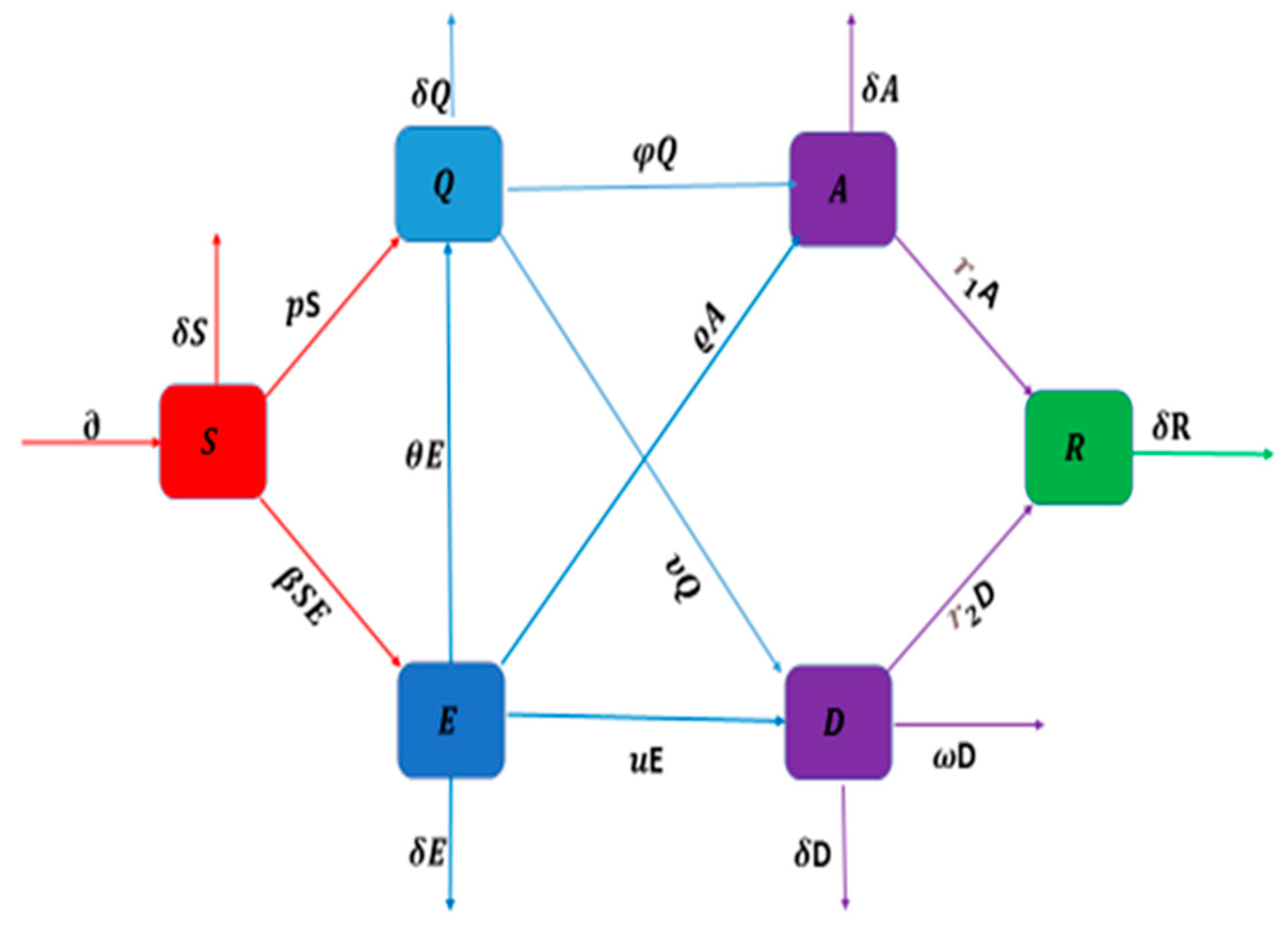
Figure 1. COVID-19 flow chart for mathematical model (1).
Fractalfract 07 00451 g001
Figure 2. Numerical simulation for model (2) using the NSFD scheme with a   h = 0.001 , b     h = 0.01 , c   h = 0.1 , and   d   h = 1 . Other parameters remain fixed: p = 0.001 ,   β = 0.1 ,   ω = 0.14 ,   θ = 0.15 , u = 0.25 , φ = 0.4 , δ = 0.3 ,   υ = 0.12 ,   ϱ = 0.35 ,   r 1 = 0.35 ,   r 2 = 0.45 , and   𝜕 = 0.2 .
Fractalfract 07 00451 g002
Figure 3. Numerical simulation for model (2) using the NSFD scheme with a h = 0.001 ,   b   h = 0.01 , c   h = 0.1 , and   d   h = 0.5 . Other parameters remain fixed: p = 0.001 ,   β = 0.1 ,   ω = 0.14 ,   θ = 0.15 , u = 0.25 ,   φ = 0.4 , δ = 0.3 ,   υ = 0.12 , ϱ = 0.35 ,   r 1 = 0.35 ,   r 2 = 0.45 , and   𝜕 = 5.2 .
Fractalfract 07 00451 g003
Table 1. Parameters and their biological descriptions.
ParametersParameters’ Description
β Rate of contact between susceptible and exposed people
𝜕 Recruitment rate of mortality
θ The rate of transmission from exposed to quarantined persons
υ The rate of transmission from quarantined to symptomatic persons
p The rate of transmission from susceptible to quarantined persons
ω The rate of mortality in symptomatic infected persons
δ The rate of natural fatality
φ The rate of transmission from quarantined to asymptomatic persons
u The rate of transmission from exposed to symptomatic persons
r 1 The rate of recovered persons from asymptomatic disease
r 2 The rate of recovered persons from symptomatic disease
ϱ Transfer rate of exposed persons to asymptomatic persons
Disclaimer/Publisher’s Note: The statements, opinions and data contained in all publications are solely those of the individual author(s) and contributor(s) and not of MDPI and/or the editor(s). MDPI and/or the editor(s) disclaim responsibility for any injury to people or property resulting from any ideas, methods, instructions or products referred to in the content.