Stability, Data Dependence, and Convergence Results with Computational Engendering of Fractals via Jungck–DK Iterative Scheme

Abstract

We have developed a Jungck version of the DK iterative scheme called the Jungck–DK iterative scheme. Our analysis focuses on the convergence and stability of the Jungck–DK scheme for a pair of non-self-mappings using the more general contractive condition. We demonstrate that this iterative scheme converges faster than all other leading Jungck-type iterative schemes. To further illustrate its effectiveness, we provide an example to verify the rate of convergence and prove the data dependence result for the Jungck–DK iterative scheme. Finally, we calculate the escape criteria for generating Mandelbrot and Julia sets for polynomial functions and present visually appealing images of these sets by our modified iteration.

1. Introduction

Fixed-point theory occupies a prominent position in both pure and applied mathematics, owing to its numerous applications in areas such as differential and integral equations, variational inequalities, approximation theory, equilibrium problems, fractal generation, and many others.

The Banach contraction theorem, introduced by Banach in 1922, is one of the fundamental results in fixed-point theory. This theorem guarantees the existence and uniqueness of fixed points for contraction mappings in metric fixed-point theory. Additionally, it allows various iterative schemes to converge to a fixed point. The theorem has also become a widely used method for solving existence problems in many mathematical fields.

While there have been numerous studies regarding fixed points of contractive maps, such as those discussed in [1,2,3,4], relatively little research has focused on the convergence of iterative approximations to these common fixed points.

When it comes to approximating fixed points, the well-known Banach contraction theorem employs the Picard iteration method. However, in many cases, obtaining the exact solution to a fixed-point problem is infeasible. Hence, as a result, a wide range of iterative algorithms have been developed and studied for approximating solutions to fixed-point problems [5,6,7,8,9,10,11,12,13,14].

The investigation of iterative methods for approximating fixed points using various types of self-mappings has gained significant attention in recent years. Researchers have introduced several iterative schemes and studied their qualitative features, including convergence, stability, and data dependency. However, non-self-mappings are typically more intricate than self-mappings and are therefore often overlooked in many cases [5,6,7].

Jungck introduced the Jungck iteration scheme [15] to approximate the fixed points for the non-self-mapping $\mathcal{U}$, $\mathcal{V}:\mathcal{A}\to \mathcal{W},$ where $\mathcal{W}$ is a Banach space and $\mathcal{A}$ is an arbitrary set such that $\mathcal{V}\left(\mathcal{A}\right)\subseteq \mathcal{U}\left(\mathcal{A}\right)$ satisfies the following Jungck contraction:

$$\begin{array}{cc}\hfill d(\mathcal{V}u,\mathcal{V}v)& \le \alpha d(\mathcal{U}u,\mathcal{U}v),0\le \alpha <1.\hfill \end{array}$$

(1)

In 2005, the Jungck–Mann iteration scheme and its stability for two contractive maps were first presented and discussed by Singh et al. [12]. Within this framework, Olatinwo and Imoru [8] and Olatinwo [16,17] introduced the Jungck–Ishikawa and Noor iteration schemes and exhibited how their convergence could be utilised for pairs of some generalized contractive operator for approximating the common fixed point. Chugh and Kumar [9] presented the Jungck–SP iterative scheme, which is defined as follows:

$$\begin{array}{cc}\hfill \mathcal{U}{u}_{n+1}=& (1-{\rho }_n)\mathcal{U}{v}_n+{\rho }_n\mathcal{V}{v}_n\hfill \\ \hfill \mathcal{U}{v}_n=& (1-{\varrho }_n)\mathcal{U}{w}_n+{\varrho }_n\mathcal{V}{w}_n\hfill \\ \hfill \mathcal{U}{w}_n=& (1-{\sigma }_n)\mathcal{U}{u}_n+{\sigma }_n\mathcal{V}{u}_n,\hfill \end{array}$$

(2)

where ${\rho }_n,{\varrho }_n,{\sigma }_n$ are in $[0,1]$.

Nawab Hussain et al. [10] presented the Jungck–CR scheme and used the more general contractive condition of Olatino [16] to prove the stability, data dependency, and convergence of the Jungck–CR iterative scheme. The general contractive condition of Olatino [16] is defined as follows:

Let $r\in [0,1)$ be a real number and let $\lambda :{\mathbb{R}}^{+}\to {\mathbb{R}}^{+}$ be a monotone function such that $\lambda \left(0\right)=0$. If, for all $u,v$ belongs to A, we have

$$\begin{array}{cc}\hfill \parallel \mathcal{V}u-\mathcal{V}v\parallel & \le \lambda (\parallel \mathcal{U}u-\mathcal{V}u\parallel )+r\parallel \mathcal{U}u-\mathcal{U}v\parallel .\hfill \end{array}$$

(3)

The Jungck–CR iterative scheme is defined by the sequence $\left\{u_n\right\}$

$$\begin{array}{cc}\hfill \mathcal{U}{u}_{n+1}=& (1-{\rho }_n)\mathcal{U}{v}_n+{\rho }_n\mathcal{V}{v}_n\hfill \\ \hfill \mathcal{U}{v}_n=& (1-{\varrho }_n)\mathcal{V}{u}_n+{\varrho }_n\mathcal{V}{w}_n\hfill \\ \hfill \mathcal{U}{w}_n=& (1-{\sigma }_n)\mathcal{U}{u}_n+{\sigma }_n\mathcal{V}{u}_n,\hfill \end{array}$$

(4)

where ${\rho }_n,{\varrho }_n,$ and ${\sigma }_n$ are sequences of positive numbers in $[0,1]$.

Motivated by the above literature, we propose the following Jungck type iterative scheme. For ${\rho }_n,{\varrho }_n\in [0,1],$ we have

$$\begin{array}{cc}\hfill \mathcal{U}{u}_{n+1}=& (1-{\rho }_n)\mathcal{U}{w}_n+{\rho }_n\mathcal{V}{v}_n\hfill \\ \hfill \mathcal{U}{v}_n=& (1-{\varrho }_n)\mathcal{U}{u}_n+{\varrho }_n\mathcal{V}{w}_n\hfill \\ \hfill \mathcal{U}{w}_n=& \mathcal{V}{u}_n\hfill \end{array}$$

(5)

which we call the Jungck–DK iterative scheme.

In this paper, we present the Jungck–DK iterative scheme for analyzing the convergence and stability of a non-self-mapping in a normed linear space. Our work is motivated by previous research in the field. To demonstrate the superior convergence rate of the Jungck–DK iterative scheme compared to other Jungck-type iterative schemes, we provide an example. Additionally, we prove data dependence results. In the final section, we showcase the practical application of the Jungck–DK iterative scheme by generating Mandelbrot and Julia sets of polynomial functions for visualizing images on both sets.

2. Preliminaries

In this section, we set out some lemmas, propositions, and definitions that are used in this paper.

Definition 1

([18]). Suppose that $\left\{x_n\right\}$ and $\left\{y_n\right\}$ are two real convergent sequences with limits x and y, respectively. Then, $\left\{x_n\right\}$ is said to converge faster than $\left\{y_n\right\}$ if

$$\begin{array}{c}\hfill \underset{n\to \infty }{lim}\left|\frac{x_n-x}{y_n-y}\right|=0.\end{array}$$

Definition 2

([19]). Let $f_1$ and $f_2$ be two self-maps on $\mathcal{W}$. A point u in $\mathcal{W}$ is called the coincidence point of a pair of mappings $(f_1,f_2)$ if $f_{1}u=f_{2}u$ and a common fixed point of a pair $(f_1,f_2)$ if $u=f_{1}u=f_{2}u$. If $v=f_{1}u=f_{2}u$ for some $u\in \mathcal{W}$, then the point v is coincident point of $f_1$ and $f_2$. A pair $(f_1,f_2)$ is weakly compatible if $f_1$ & $f_2$ commute at v.

Lemma 1

([11]). If $\upsilon \in \mathbb{R}$ such that $0\le \upsilon <1$ and $\left\{{\epsilon }_{}\right\}$ is a sequence of positive numbers such that $\underset{n\to \infty }{lim}{\epsilon }_n=0,$ then for any sequence of positive numbers $\left\{a_n\right\}$ satisfying

$$a_{n+1}\le \upsilon a_n+{\epsilon }_n,n=0,1,2,\dots ,$$

one has $\underset{n\to \infty }{lim}{a}_n=0.$

Definition 3

([12]). Let $\mathcal{U},\mathcal{V}:\mathcal{A}\to \mathcal{W}$ be two non-self operators for an arbitrary set $\mathcal{A}$ such that $\mathcal{V}\left(\mathcal{A}\right)\subseteq \mathcal{U}\left(\mathcal{A}\right)$ and $g^{*}$ is a point of coincidence of $\mathcal{U}$ and $\mathcal{V}.$ Let $\mathcal{U}{u}_n\subset \mathcal{W},$ be the sequence generated by an iterative scheme

$$\mathcal{U}{u}_{n+1}=f(\mathcal{V},u_n),n=0,1,2,\dots ,$$

where $u_0\in \mathcal{W}$ is the initial approximation and f is some function. Suppose that $\left\{\mathcal{U}{u}_n\right\}$ converges to $g^{*}$. If $\left\{\mathcal{U}{v}_n\right\}\subset \mathcal{W}$ is an arbitrary sequence and if ${\epsilon }_n=d(\mathcal{U}{v}_n,f(\mathcal{V},u_n)),n=0,1,2,\dots$, then the defined iterative scheme is said to be stable or $(\mathcal{U},\mathcal{V})-$ stable ⇔$\underset{n\to \infty }{lim}{\epsilon }_n=0$⇒ $\underset{n\to \infty }{lim}\mathcal{U}{v}_n=g^{*}.$

Ostrowski [13] found the first stability result for T-stable mappings in 1967, when he talked about the stability of the Picard iteration using the contraction mapping. Harder [14] established how stability results can be used to solve first-order differential equations. Osilike and Udomene [20] came up with a shorter method to show that results are stable. Berinde [21], Imoru and Olatinwo [16], and many others (see [8,9,10]) have also used this method.

Definition 4

([22]). Consider two self-operators $S,S_1:\mathcal{W}\to \mathcal{W}$ and let $S_1$ be an appropriate operator of S if, for all $u\in \mathcal{W}$ and for a fixed $\epsilon >0,$ we have

$$\parallel Su-S_{1}u\parallel \le \epsilon .$$

Lemma 2

([22]). Let $\left\{a_n\right\}$ be a sequence in ${\mathbb{R}}_{+}\cup \left\{0\right\}$, and let $n,n_0\in \mathbb{N}$ be a number such that for every $n\ge n_0$, the following inequality holds:

$$a_{n+1}\le (1-p_n)a_n+p_n{q}_n,\forall n\in \mathbb{N},$$

where $p_n\in (0,1)$, ${\displaystyle \sum _{n=1}^{\infty }}{p}_n=\infty$ and $q_n\ge 0,for all n\in \mathbb{N}$. Then, $0\le \underset{n\to \infty }{lim\; sup}{a}_n\le \underset{n\to \infty }{lim\; sup}{q}_n$.

3. Convergence, Data Dependence, and Stability in an Arbitrary Banach Space

This section deals with the convergence, stability, and data dependence of the Jungck–DK iterative scheme.

Theorem 1.

Let $\mathcal{A}$ be an arbitrary set of an arbitrary Banach space $(\mathcal{W},|·\left|\right)$ and let there be two non-self-operators $\mathcal{U},\mathcal{V}:\mathcal{A}\to \mathcal{W}$, which satisfy the condition (3). Consider $\mathcal{V}\left(\mathcal{A}\right)\subseteq \mathcal{V}\left(\mathcal{A}\right)$, where $\mathcal{V}\left(\mathcal{A}\right)$ is a complete subspace of $\mathcal{W}$ and $\mathcal{U}\left(p\right)=\mathcal{V}\left(p\right)=u^{*}$ (say). For $u_0\in \mathcal{A},$ a sequence $\left\{\mathcal{U}\left(u_n\right)\right\}$ is the sequence of the Jungck–DK iterative scheme defined by (5), where $0\le {\rho }_n,{\varrho }_n,{\sigma }_n\le 1$, with $\left\{{\rho }_n\right\}$ satisfying ${\displaystyle \sum _{n=0}^{\infty }}\left\{{\rho }_n\right\}<\infty$. Then, the scheme (5) converges strongly to $u^{*}$. Moreover, if $\mathcal{A}=\mathcal{W}$ with $\mathcal{U}$ and $\mathcal{V}$ satisfy the weak compatibility property, then $u^{*}$ is also a unique common fixed point of both operators.

Proof. 

In the beginning, we demonstrated that the Jungck–DK iterative scheme (5) converges to $u^{*}$, where $u^{*}$ is a fixed point of $\mathcal{U}$ and $\mathcal{V}$.

From (5)

$$\begin{array}{cc}\hfill \parallel \mathcal{U}{u}_{n+1}-u^{*}\parallel =& \parallel (1-{\rho }_n)\mathcal{U}{w}_n+{\rho }_n\mathcal{V}{v}_n-u^{*}\parallel \hfill \end{array}$$

$$\begin{array}{cc}\hfill \le & (1-{\rho }_n)\parallel \mathcal{U}{w}_n-u^{*}\parallel +{\rho }_n\parallel \mathcal{V}{v}_n-u^{*}\parallel \hfill \\ \hfill \parallel \mathcal{V}{v}_n-u^{*}\parallel =& \parallel \mathcal{V}{v}_n-\mathcal{V}p\parallel \hfill \\ \hfill \le & \lambda (\parallel \mathcal{U}p-\mathcal{V}p\parallel )+r\parallel \mathcal{U}p-\mathcal{U}{v}_n\parallel \hfill \\ \hfill \le & r\parallel \mathcal{U}p-\mathcal{U}{v}_n\parallel \hfill \end{array}$$

(6)

$$\begin{array}{cc}\hfill =& r\parallel \mathcal{U}{v}_n-u^{*}\parallel .\hfill \\ \hfill \parallel \mathcal{U}{v}_n-u^{*}\parallel =& \parallel (1-{\varrho }_n)\mathcal{U}{u}_n+{\varrho }_n\mathcal{V}{w}_n-u^{*}\parallel \hfill \end{array}$$

(7)

$$\begin{array}{cc}\hfill \le & (1-{\varrho }_n)\parallel \mathcal{U}{u}_n-u^{*}\parallel +{\varrho }_n\parallel \mathcal{V}{w}_n-u^{*}\parallel \hfill \\ \hfill \parallel \mathcal{V}{w}_n-u^{*}\parallel =& \parallel \mathcal{V}p-\mathcal{V}{w}_n\parallel \hfill \\ \hfill \le & \lambda (\parallel \mathcal{U}p-\mathcal{V}p\parallel )+r\parallel \mathcal{U}p-\mathcal{U}{w}_n\parallel \hfill \\ \hfill \le & r\parallel \mathcal{U}p-\mathcal{U}{w}_n\parallel \hfill \end{array}$$

(8)

$$\begin{array}{cc}\hfill =& r\parallel \mathcal{U}{w}_n-u^{*}\parallel \hfill \end{array}$$

(9)

$$\begin{array}{cc}\hfill \parallel \mathcal{U}{w}_n-u^{*}\parallel =& \parallel \mathcal{V}{u}_n-\mathcal{V}p\parallel \hfill \\ \hfill \le & \lambda (\parallel \mathcal{U}p-\mathcal{V}p\parallel )+r\parallel \mathcal{U}p-\mathcal{U}{u}_n\parallel \hfill \\ \hfill \le & r\parallel \mathcal{U}p-\mathcal{U}{u}_n\parallel \hfill \\ \hfill =& r\parallel \mathcal{U}{u}_n-u^{*}\parallel .\hfill \end{array}$$

(10)

From (10) and (9), we have

$$\parallel \mathcal{V}{w}_n-u^{*}\parallel \le r^2\parallel \mathcal{U}{u}_n-u^{*}\parallel .$$

(11)

Replacing (11) in (8) we obtain

$$\begin{array}{cc}\hfill \parallel \mathcal{U}{v}_n-\mathcal{U}{u}^{*}\parallel \le & (1-{\varrho }_n)\parallel \mathcal{U}{u}_n-u^{*}\parallel +{\varrho }_n{r}^2\parallel \mathcal{U}{u}_n-u^{*}\parallel \hfill \\ \hfill \le & (1-{\varrho }_n(1-r^2))\parallel \mathcal{U}{u}_n-u^{*}\parallel .\hfill \end{array}$$

(12)

Equation (7) implies

$$\parallel \mathcal{V}{u}_n-u^{*}\parallel \le r(1-{\varrho }_n(1-r^2))\parallel \mathcal{U}{u}_n-u^{*}\parallel .$$

(13)

From Equation (6), we obtain

$$\begin{array}{cc}\hfill \parallel \mathcal{U}{u}_{n+1}-u^{*}\parallel \le & (1-{\rho }_n)r\parallel \mathcal{U}{u}_n-u^{*}\parallel +{\rho }_{n}r(1-{\varrho }_n(1-r^2))\parallel \mathcal{U}{u}_n-u^{*}\parallel \hfill \\ \hfill \le & r(1-{\rho }_n(1-(1-{\varrho }_n(1-r^2))))\parallel \mathcal{U}{u}_n-u^{*}\parallel \hfill \\ \hfill \le & r\prod _{k=0}^n(1-{\rho }_k(1-{\varrho }_k(1-r^2)))\parallel \mathcal{U}{u}_0-u^{*}\parallel \hfill \\ \hfill \le & e^{-(1-(1-{\varrho }_k(1-r^2))){\Sigma }_{k=0}^{\infty }{\rho }_k}\parallel \mathcal{U}{u}_0-u^{*}\parallel .\hfill \end{array}$$

(14)

Since $0\le r<1,$${\rho }_k\in [0,1]$ and $\sum _{k=0}^{\infty }{\rho }_k=\infty$, therefore,

$$e^{-(1-(1-{\varrho }_k(1-r^2)))\sum _{k=0}^{\infty }{\rho }_k}\to 0\mathrm{as}n\to \infty .$$

As a result, it follows from (14) that

$$\underset{n\to \infty }{lim}\parallel \mathcal{U}{u}_{n+1}-u^{*}\parallel =0.$$

Consequently, $\left\{\mathcal{U}{u}_n\right\}\to u^{*}.$

Next, our claim is to show that $u^{*}$ is a unique common fixed point of $\mathcal{U}$ and $\mathcal{V}$. We consider that $u^{**}$ is also a coincidence point. Then, there is $v^{*}\in \mathcal{W}$ such that $\mathcal{U}{v}^{*}=\mathcal{V}{v}^{*}=u^{**}$. However, according to (3), we have

$$\begin{array}{cc}\hfill 0\le \parallel u^{*}-u^{**}\parallel =& \parallel \mathcal{V}v-\mathcal{V}{v}^{*}\parallel \hfill \\ \hfill \le & \lambda (\parallel \mathcal{U}v-\mathcal{V}v\parallel )+r\parallel \mathcal{U}v-\mathcal{U}{v}^{*}\parallel \hfill \\ \hfill =& r\parallel u^{*}-u^{**}\parallel ,\hfill \end{array}$$

which means that $u^{*}=u^{**}$ as $0\le r<1.$

Since $\mathcal{U}$ and $\mathcal{V}$ are weakly compatible with $u^{*}=\mathcal{V}v=\mathcal{U}v$ (so $\mathcal{V}{u}^{*}=\mathcal{VV}v=\mathcal{VU}v=\mathcal{UV}v$ and hence $\mathcal{V}{u}^{*}=\mathcal{U}{u}^{*}$), $\mathcal{V}{u}^{*}$ is a point of coincidence of $\mathcal{U}$ and $\mathcal{V}$, which is unique. Then, $u^{*}=\mathcal{V}{u}^{*}$. Thus, $\mathcal{U}{u}^{*}=\mathcal{V}{u}^{*}=u^{*}$, and both $\mathcal{U}$ and $\mathcal{V}$ shared a unique fixed point $u^{*}$.    □

The next result deals with the stability of the Jungck–DK-type iterative scheme (5).

Theorem 2.

Let $\mathcal{U},\mathcal{V}$, and $\left\{u_n\right\}$ satisfy all the hypotheses and requirements of Theorem 1. Then, the Jungck–DK scheme (5) is $(\mathcal{U},\mathcal{V})$-stable.

Proof. 

Suppose there is an arbitrary sequence $\left\{j_n\right\}\subset \mathcal{W}$, ${\epsilon }_n=\parallel \mathcal{U}{j}_{n+1}-(1-{\rho }_n)\mathcal{U}{b}_n-{\rho }_n\mathcal{V}{a}_n\parallel$ for $n=0,1,2,\dots ,$ where $\mathcal{U}{a}_n=(1-{\varrho }_n)\mathcal{U}{j}_n+{\varrho }_n\mathcal{V}{b}_n$ and $\mathcal{U}{b}_n=\mathcal{V}{j}_n$. Let $\underset{n\to \infty }{lim}{\epsilon }_n=0.$

Then, from the Jungck–DK iterative scheme (5), we have

$$\begin{array}{cc}\hfill \parallel \mathcal{U}{j}_{n+1}-u^{*}\parallel \le & \parallel \mathcal{U}{j}_{n+1}-(1-{\rho }_n)\mathcal{U}{b}_n-{\rho }_n\mathcal{V}{a}_n\parallel +\parallel (1-{\rho }_n)\mathcal{U}{b}_n-{\rho }_n\mathcal{V}{a}_n-u^{*}\parallel \hfill \\ \hfill \le & {\epsilon }_n+(1-{\rho }_n)\parallel \mathcal{U}{b}_n-u^{*}\parallel +{\rho }_n\parallel \mathcal{V}{a}_n-u^{*}\parallel \hfill \\ \hfill \le & {\epsilon }_n+(1-{\rho }_n)\parallel \mathcal{U}{b}_n-u^{*}\parallel +{\rho }_{n}r\parallel \mathcal{U}{a}_n-u^{*}\parallel .\hfill \end{array}$$

(15)

$$\begin{array}{cc}\hfill \parallel \mathcal{U}{b}_n-u^{*}\parallel =& \parallel \mathcal{V}{j}_n-\mathcal{V}p\parallel \hfill \\ \hfill \le & \lambda (\parallel \mathcal{U}p-\mathcal{V}p\parallel )+r\parallel \mathcal{U}p-\mathcal{U}{j}_n\parallel \hfill \\ \hfill \le & r\parallel \mathcal{U}{j}_n-u^{*}\parallel .\hfill \end{array}$$

(16)

$$\begin{array}{cc}\hfill \parallel \mathcal{U}{a}_n-u^{*}\parallel =& \parallel (1-{\varrho }_n)\mathcal{U}{j}_n+{\varrho }_n\mathcal{V}{b}_n-u^{*}\parallel \hfill \\ \hfill \le & (1-{\varrho }_n)\parallel \mathcal{U}{j}_n-u^{*}\parallel +{\varrho }_n\parallel \mathcal{V}{b}_n-\mathcal{V}p\parallel \hfill \\ \hfill \le & (1-{\varrho }_n)\parallel \mathcal{U}{j}_n-u^{*}\parallel +r{\varrho }_n\parallel \mathcal{U}{j}_n-u^{*}\parallel \hfill \\ \hfill \le & (1-{\varrho }_n(1-r^2))\parallel \mathcal{U}{j}_n-u^{*}\parallel .\hfill \end{array}$$

(17)

Putting (17) & (16) in (15), we obtain

$$\begin{array}{cc}\hfill \parallel \mathcal{U}{j}_{n+1}-u^{*}\parallel \le & {\epsilon }_n+(1-{\rho }_n)r\parallel \mathcal{U}{j}_n-u^{*}\parallel +{\rho }_{n}r(1-{\varrho }_n(1-r^2))|\mathcal{U}{j}_n-u^{*}\parallel \hfill \\ \hfill \le & {\epsilon }_n+r(1-{\rho }_n(1-(1-{\varrho }_n(1-r^2))))\parallel \mathcal{U}{j}_n-u^{*}\parallel .\hfill \end{array}$$

Using that $\rho \le {\rho }_n$ and $r\in [0,1)$, we have

$$\left[r(1-{\rho }_n(1-(1-{\varrho }_n(1-r^2))))\right]<1.$$

Hence, using Lemma 1 implies

$$\underset{n\to \infty }{lim}\mathcal{U}{j}_{n+1}=u^{*}.$$

Conversely, let us consider that $\underset{n\to \infty }{lim}\mathcal{U}{j}_{n+1}=u^{*}$. Then, using the condition (3) and the triangular inequality, we have

$$\begin{array}{cc}\hfill {\epsilon }_n=& \parallel \mathcal{U}{j}_{n+1}-(1-{\rho }_n)\mathcal{U}{b}_n-{\rho }_n\mathcal{V}{a}_n\parallel \hfill \\ \hfill \le & \parallel \mathcal{U}{j}_{n+1}-u^{*}\parallel +(1-{\rho }_n)\parallel \mathcal{U}{b}_n-u^{*}\parallel +{\rho }_n\parallel \mathcal{V}{a}_n-u^{*}\parallel .\hfill \end{array}$$

From (17) & (16), we obtain

$${\epsilon }_n\le \parallel \mathcal{U}{j}_{n+1}-u^{*}\parallel +r(1-{\rho }_n(1-(1-{\varrho }_n(1-r^2))))\parallel \mathcal{U}{j}_n-u^{*}\parallel .$$

Hence, $\underset{n\to \infty }{lim}{\epsilon }_n=0$⇒ the Jungck–DK scheme is $(\mathcal{U},\mathcal{V})$- stable.    □

In the next theorem, we will compare the convergence behaviour of the Jungck–DK-type iterative scheme (5) with the Jungck–CR-type iterative scheme, which converges faster than all Jungck-type (Picard, Mann, Ishikawa, Noor, S, and SP) iterative schemes.

Theorem 3.

Let $\mathcal{U},\mathcal{V}$, and $\left\{u_n\right\}$ satisfy all the hypotheses of Theorem 1. For $u_0\in \mathcal{A}$, the Jungck–DK scheme (5) converges faster than the Jungck–CR scheme (4) to a fixed point $u^{*}.$

Proof. 

Let $u^{*}=\mathcal{U}\left(p\right)=\mathcal{V}\left(p\right)$ (say). By using the contractive condition (3), and from the iterative scheme of Jungck–CR [10], we have

$$\parallel \mathcal{U}{u}_{n+1}-u^{*}\parallel \le r(1-{\rho }_n(1-r))\parallel \mathcal{U}{u}_n-u^{*}\parallel =b_n.$$

Additionally, from Theorem 1 of the Jungck–DK iterative scheme, we have

$$\parallel \mathcal{U}{u}_{n+1}-u^{*}\parallel \le r(1-{\rho }_n(1-(1-{\varrho }_n(1-r^2))))\parallel \mathcal{U}{u}_n-u^{*}\parallel =a_n.$$

Now,

$$\begin{array}{cc}\hfill \frac{a_n}{b_n}=& \prod _{i=0}^n\left[\frac{r(1-{\rho }_i(1-(1-{\varrho }_i(1-r^2))))}{r(1-{\rho }_i(1-r))}\right]\parallel \mathcal{U}{u}_0-u^{*}\parallel \hfill \\ \hfill \frac{a_n}{b_n}=& \prod _{i=0}^n\left[\frac{1-{\rho }_i(1-(1-{\varrho }_i(1-r^2))))}{1-{\rho }_i(1-r)}\right]\parallel \mathcal{U}{u}_0-u^{*}\parallel .\hfill \end{array}$$

(18)

Since $r\in [0,1)$, $\underset{n\to \infty }{lim}{\rho }_n=0=\underset{n\to \infty }{lim}{\varrho }_n$. Hence, from (18), we have

$$\underset{n\to \infty }{lim}\parallel \frac{a_n}{b_n}\parallel \to 0.$$

In conclusion, the Jungck–DK iterative scheme converges faster than the Jungck–CR scheme.    □

The previous Theorem 3 can be demonstrated by the following example.

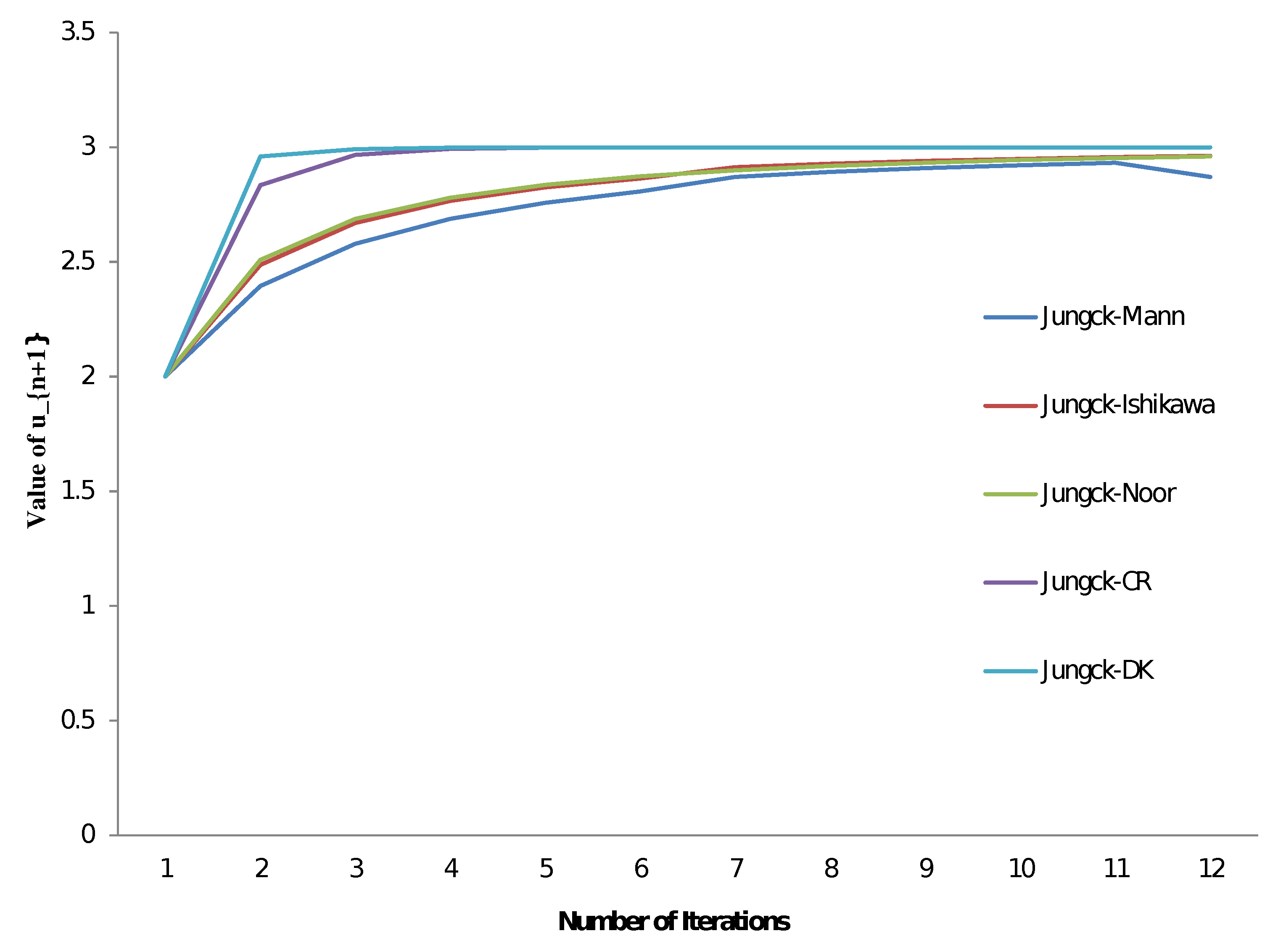
Example 1.

Consider $\mathcal{U},\mathcal{V}:[1,4]\to [1,16]$ such that $\mathcal{V}u=2u+3$ and $\mathcal{U}u=u^2.$ It is not difficult to remark that $\mathcal{U}$ and $\mathcal{V}$ are two quasi-contractive operators accomplishing the (3) condition, with 9 as their coincidence point. Take $u_0=2$ as the initial approximation; then, with $\lambda \left(t\right)=2at$ and ${\rho }_n={\varrho }_n={\sigma }_n=\frac{1}{\sqrt{2n+1}},n\ge 0$, we construct

Table 1. Convergence of various Jungck-type schemes to the coincidence point $u^{*}=9=\mathcal{V}3=\mathcal{U}3$, $u_0=2$, ${\rho }_n={\varrho }_n=\frac{1}{\sqrt{2n+1}}$.

n	Jungck–Mann Iterative Scheme			Jungck–Ishikawa Iterative Scheme			Jungck–Noor Iterative Scheme			Jungck–CR Iterative Scheme			Jungck–DK Iterative Scheme
	$\mathcal{V}{\mathit{u}}_{\mathit{n}}$	$\mathcal{U}{\mathit{u}}_{\mathit{n}}$	${\mathit{u}}_{\mathit{n}+\mathit{1}}$	$\mathcal{V}{\mathit{u}}_{\mathit{n}}$	$\mathcal{U}{\mathit{u}}_{\mathit{n}}$	${\mathit{u}}_{\mathit{n}+\mathit{1}}$	$\mathcal{V}{\mathit{u}}_{\mathit{n}}$	$\mathcal{U}{\mathit{u}}_{\mathit{n}}$	${\mathit{u}}_{\mathit{n}+\mathit{1}}$	$\mathcal{V}{\mathit{u}}_{\mathit{n}}$	$\mathcal{U}{\mathit{u}}_{\mathit{n}}$	${\mathit{u}}_{\mathit{n}+\mathit{1}}$	$\mathcal{V}{\mathit{u}}_{\mathit{n}}$	$\mathcal{U}{\mathit{u}}_{\mathit{n}}$	${\mathbf{u}}_{\mathit{n}+\mathit{1}}$
0	7.00000	4.00000	2.39417	7.00000	4.00000	2.48741	7.00000	4.00000	2.50896	7.00000	4.00000	2.83474	7.00000	4.00000	2.95956
1	7.78834	5.73205	2.57908	7.97482	6.18720	2.66946	8.01791	6.29486	2.68722	8.66949	8.03578	2.96628	8.91912	8.75900	2.99051
2	8.15816	6.65165	2.68720	8.33892	7.12601	2.76556	8.37444	7.22116	2.77952	8.93255	8.79879	2.99238	8.98102	8.94315	2.99740
3	8.37441	7.22106	2.75781	8.53113	7.64835	2.82449	8.55903	7.72571	2.83556	8.98476	8.95435	2.99817	8.99480	8.98441	2.99924
4	8.51562	7.60551	2.80712	8.64898	7.97774	2.86384	8.67111	8.04039	2.87276	8.99634	8.98903	2.99954	8.99848	8.99544	2.99976
5	8.68633	8.08358	2.87040	8.78328	8.36157	2.91207	8.74553	8.25277	2.89894	8.99908	8.99725	2.99988	8.99952	8.99856	2.99993
6	8.74080	8.23921	2.89152	8.82414	8.48015	2.92754	8.79787	8.40384	2.91812	8.99976	8.99929	2.99997	8.99986	8.99958	2.99998
7	8.78303	8.36086	2.90822	8.85509	8.57051	2.93954	8.83624	8.51541	2.93261	8.99994	8.99981	2.99999	8.99996	8.99988	3.00000
8	8.81643	8.45772	2.92164	8.87908	8.64090	2.94902	8.86522	8.60021	2.94383	8.99998	8.99995	3.00000	8.99998	8.99998	3.00000
9	8.84328	8.53599	2.93259	8.89804	8.69673	2.95663	8.88766	8.66612	2.95268	9.00000	8.99999	3.00000	9.00000	9.00000	3.00000
10	8.68633	8.08358	2.87040	8.78328	8.36157	2.96207	8.90536	8.71831	2.95977	9.00000	9.00000	3.00000	9.00000	9.00000	3.00000

. Studying the table, we can observe the convergence of the various Jungck0type schemes to the same point $u^{*}=9=\mathcal{V}3=\mathcal{U}3.$

Remark 1.

We find that the Jungck–DK iterative scheme converges to the coincidence point in just 8 iterations, while the Jungck–Mann iterative scheme takes 229 iterations to obtain the same results. Similarly, the Jungck–Ishikawa iterative scheme takes 205 iterations, the Jungck–Noor iterative scheme takes 200 iterations, and the Jungck–CR iterative scheme takes 10 iterations. Figure 1 provides a visual representation of our convergence comparisons.

Now, let us give a data dependence result for the Jungck–DK scheme.

Definition 5.

Let $\mathcal{A}$ be an arbitrary set of an arbitrary Banach space $(\mathcal{W},|·\left|\right)$ and let $(\mathcal{U},\mathcal{V}),({\mathcal{U}}_1,{\mathcal{V}}_1):\mathcal{A}\to \mathcal{W}$ be two non-self-operator pairs such that $\mathcal{V}\left(\mathcal{A}\right)\subseteq \mathcal{U}\left(\mathcal{A}\right)$ and ${\mathcal{V}}_1\left(\mathcal{A}\right)\subseteq {\mathcal{U}}_1\left(\mathcal{A}\right)$. The pair $(\mathcal{U},\mathcal{V})$ is called an approximative operator pair of $({\mathcal{U}}_1,{\mathcal{V}}_1)$ if, for every $u\in \mathcal{W}$ and some fixed ${ϵ}_1>0$ and ${ϵ}_2>0$, we have

$$\parallel \mathcal{V}u-{\mathcal{V}}_{1}u\parallel \le {ϵ}_1,\parallel \mathcal{U}u-{\mathcal{U}}_{1}u\parallel \le {ϵ}_2.$$

Theorem 4.

Let $(\mathcal{W},\parallel ·\parallel )$ be a Banach space, such that $(\mathcal{U},\mathcal{V}),({\mathcal{U}}_1,{\mathcal{V}}_1):\mathcal{A}\to \mathcal{W}$ satisfies condition (3), where $\mathcal{V}\left(\mathcal{A}\right)\subseteq \mathcal{U}\left(\mathcal{A}\right)$ and ${\mathcal{V}}_1\left(\mathcal{A}\right)\subseteq {\mathcal{U}}_1\left(\mathcal{A}\right)$. ${\mathcal{U}}_1\left(\mathcal{A}\right)$ is a complete subset of $\mathcal{W}$. Assume that there exists a $p\in C(\mathcal{U},\mathcal{V})$ and $p\in C({\mathcal{U}}_1,{\mathcal{V}}_1)$ such that $\mathcal{U}p=\mathcal{V}p=u^{*}$ and ${\mathcal{U}}_1{p}_1={\mathcal{V}}_1{p}_1=u^{**}.$ Let $\left\{\mathcal{U}{u}_n\right\}$ be an iterative sequence (5) with $\left\{{\rho }_n\right\},\left\{{\varrho }_n\right\}\subset [0,1]$ satisfying ${\displaystyle \sum _{n=0}^{\infty }}{\rho }_n{\varrho }_n=\infty$, and let $\left\{{\mathcal{U}}_1{a}_{n+1}\right\}$ be a sequence defined by   

$$\begin{array}{c}\hfill \left\{\begin{array}{cc}\hfill & {\mathcal{U}}_1{a}_{n+1}=(1-{\rho }_n){\mathcal{U}}_1{c}_n+{\rho }_n{\mathcal{V}}_1{b}_n\hfill \\ \hfill & {\mathcal{U}}_1{b}_n=(1-{\varrho }_n){\mathcal{U}}_1{a}_n+{\varrho }_n{\mathcal{V}}_1{c}_n\hfill \\ \hfill & {\mathcal{U}}_1{c}_n={\mathcal{V}}_1{a}_n.\hfill \end{array}\right.\end{array}$$

(19)

Assume that $\left\{\mathcal{U}{u}_{n+1}\right\}$ and $\left\{{\mathcal{U}}_1{a}_{n+1}\right\}$ converge to $u^{*}$ and $u^{**}$. Then, we have $\parallel u^{*}-u^{**}\parallel =\frac{4ϵ}{1-r^2}$, where $ϵ=max\{{ϵ}_1,{ϵ}_2\}$.

Proof. 

Using the iterative sequence (5), the iterative scheme (19), the condition (3), and Definition 5, we obtain

$$\parallel \mathcal{U}{u}_{n+1}-{\mathcal{U}}_1{a}_{n+1}\parallel \le (1-{\rho }_n)\parallel \mathcal{U}{w}_n-{\mathcal{U}}_1{c}_n\parallel +{\rho }_n\parallel \mathcal{V}{v}_n-{\mathcal{V}}_1{b}_n\parallel ,$$

(20)

$$\begin{array}{cc}\hfill \parallel \mathcal{V}{v}_n-{\mathcal{V}}_1{b}_n\parallel \le & \parallel \mathcal{V}{v}_n-\mathcal{V}{b}_n\parallel +\parallel \mathcal{V}{b}_n-{\mathcal{V}}_1{b}_n\hfill \\ \hfill \le & \parallel \mathcal{V}{v}_n-\mathcal{V}{b}_n\parallel +{ϵ}_1\hfill \\ \hfill \le & \lambda \parallel \mathcal{U}{v}_n-\mathcal{V}{v}_n\parallel +r\parallel \mathcal{U}{v}_n-\mathcal{U}{b}_n\parallel +{ϵ}_1\hfill \\ \hfill \le & \lambda \parallel \mathcal{U}{v}_n-\mathcal{V}{v}_n\parallel +r\{\parallel \mathcal{U}{v}_n-{\mathcal{U}}_1{b}_n\parallel +\parallel {\mathcal{U}}_1{b}_n-\mathcal{U}{b}_n\parallel \}+{ϵ}_1\hfill \\ \hfill \le & \lambda \parallel \mathcal{U}{v}_n-\mathcal{V}{v}_n\parallel +r\parallel \mathcal{U}{v}_n-{\mathcal{U}}_1{b}_n\parallel +r{ϵ}_2+{ϵ}_1,\hfill \end{array}$$

(21)

$$\begin{array}{cc}\hfill \parallel \mathcal{U}{v}_n-\mathcal{V}{y}_n\parallel \le & \parallel \mathcal{U}{v}_n-\mathcal{U}p\parallel +\parallel \mathcal{V}p-\mathcal{V}{y}_n\parallel \hfill \\ \hfill \le & \parallel \mathcal{U}{v}_n-u^{*}\parallel +\lambda (\parallel \mathcal{U}p-\mathcal{V}p\parallel )+r\parallel \mathcal{U}p-\mathcal{U}{y}_n\parallel \hfill \\ \hfill \le & (1+r)\parallel \mathcal{U}{v}_n-u^{*}\parallel .\hfill \end{array}$$

It is easy to show that $\parallel \mathcal{U}{v}_n-u^{*}\parallel \le \parallel \mathcal{U}{u}_n-u^{*}\parallel$, which implies

$$\parallel \mathcal{U}{v}_n-\mathcal{V}{y}_n\parallel \le (1+r)\parallel \mathcal{U}{u}_n-u^{*}\parallel .$$

(22)

$$\begin{array}{cc}\hfill \parallel \mathcal{U}{v}_n-{\mathcal{U}}_1{b}_n\parallel \le & (1-{\varrho }_n)\parallel \mathcal{U}{u}_n+{\varrho }_n\mathcal{V}{w}_n-(1-{\varrho }_n){\mathcal{U}}_1{a}_n-{\varrho }_n\mathcal{V}{c}_n\parallel \hfill \\ \hfill \le & (1-{\varrho }_n\parallel \mathcal{U}{u}_n-{\mathcal{U}}_1{a}_n\parallel +{\varrho }_n\parallel \mathcal{V}{w}_n-{\mathcal{V}}_1{c}_n\parallel \hfill \\ \hfill \le & (1-{\varrho }_n)\parallel \mathcal{U}{u}_n-{\mathcal{U}}_1{a}_n\parallel +{\varrho }_n\{\parallel \mathcal{V}{w}_n-\mathcal{V}{c}_n\parallel +\parallel \mathcal{V}{c}_n-{\mathcal{V}}_1{c}_n\parallel \}\hfill \\ \hfill \le & (1-{\varrho }_n)\parallel \mathcal{U}{u}_n-{\mathcal{U}}_1{a}_n\parallel +{\varrho }_n\{\lambda \parallel \mathcal{U}{w}_n-\mathcal{V}{w}_n\parallel +r\parallel \mathcal{U}{w}_n-\mathcal{U}{c}_n\parallel +{ϵ}_1\}\hfill \\ \hfill \le & (1-{\varrho }_n)\parallel \mathcal{U}{u}_n-{\mathcal{U}}_1{a}_n\parallel +{\varrho }_n\{\lambda \parallel \mathcal{U}{w}_n-\mathcal{V}{w}_n\parallel +r(\parallel \mathcal{U}{w}_n-{\mathcal{U}}_1{c}_n\parallel \hfill \\ & +\parallel {\mathcal{U}}_1{c}_n-\mathcal{U}{c}_n\parallel )+{ϵ}_1\}\hfill \\ \hfill \le & (1-{\varrho }_n)\parallel \mathcal{U}{u}_n-{\mathcal{U}}_1{a}_n\parallel +{\varrho }_n\lambda \parallel \mathcal{U}{w}_n-\mathcal{V}{w}_n\parallel +{\varrho }_{n}r\parallel \mathcal{U}{w}_n-{\mathcal{U}}_1{c}_n\parallel +r{\varrho }_n{ϵ}_2+{\varrho }_n{ϵ}_1\}\hfill \\ \hfill \le & (1-{\varrho }_n)\parallel \mathcal{U}{u}_n-{\mathcal{U}}_1{a}_n\parallel +{\varrho }_n\lambda \parallel \mathcal{U}{w}_n-\mathcal{V}{w}_n\parallel +{\varrho }_{n}r\parallel \mathcal{U}{w}_n-{\mathcal{U}}_1{c}_n\parallel +r{\varrho }_n({ϵ}_1+r{ϵ}_2).\hfill \end{array}$$

(23)

Next, we consider the following estimation:

$$\begin{array}{cc}\hfill \parallel \parallel \mathcal{U}{w}_n-{\mathcal{U}}_1{c}_n\parallel =& \parallel \mathcal{V}{u}_n-{\mathcal{V}}_1{a}_n\parallel \hfill \\ \hfill \le & \parallel \mathcal{V}{u}_n-\mathcal{V}{a}_n\parallel +\parallel \mathcal{V}{a}_n-{\mathcal{V}}_1{a}_n\parallel \hfill \\ \hfill \le & \lambda (\parallel \mathcal{U}{u}_n-\mathcal{V}{u}_n\parallel )+r\parallel \mathcal{U}{u}_n-\mathcal{U}{a}_n\parallel +{ϵ}_1\hfill \\ \hfill \le & \lambda (\parallel \mathcal{U}{u}_n-\mathcal{V}{u}_n\parallel )+r\parallel \mathcal{U}{u}_n-{\mathcal{U}}_1{a}_n\parallel +r{ϵ}_2+{ϵ}_1\hfill \\ \hfill \le & \lambda \{\parallel \mathcal{U}{u}_n-u^{*}\parallel +\parallel \mathcal{V}p-\mathcal{V}{u}_n\parallel \}+r\parallel \mathcal{U}{u}_n-{\mathcal{U}}_1{a}_n\parallel +r{ϵ}_2+{ϵ}_1\hfill \\ \hfill \le & \lambda \{\parallel \mathcal{U}{u}_n-u^{*}\parallel +\parallel \mathcal{V}p-\mathcal{V}{u}_n\parallel \}+r\parallel \mathcal{U}{u}_n-\hfill \\ & {\mathcal{U}}_1{a}_n\parallel +r{ϵ}_2+{ϵ}_1\hfill \\ \hfill \le & \lambda \{\parallel \mathcal{U}{u}_n-u^{*}\parallel +\lambda \parallel \mathcal{U}p-\mathcal{V}p\parallel +r\parallel \mathcal{U}p-\mathcal{U}{u}_n\parallel \}+r\parallel \mathcal{U}{u}_n-{\mathcal{U}}_1{a}_n\parallel +r{ϵ}_2+{ϵ}_1\hfill \\ \hfill \le & (\lambda +r)\parallel \mathcal{U}{u}_n-u^{*}\parallel +r\parallel \mathcal{U}{u}_n-{\mathcal{U}}_1{a}_n\parallel +r{ϵ}_2+{ϵ}_1,\hfill \end{array}$$

(24)

$$\begin{array}{cc}\hfill \parallel \mathcal{U}{u}_n-\mathcal{V}{u}_n\parallel \le & \parallel \mathcal{U}{w}_n-\mathcal{U}p\parallel +\parallel \mathcal{V}p-\mathcal{V}{w}_n\parallel \hfill \\ \hfill \le & \parallel \mathcal{U}{w}_n-u^{*}\parallel +\lambda \parallel \mathcal{U}p-\mathcal{V}p\parallel +r\parallel \mathcal{U}p-\mathcal{U}{w}_n\parallel \hfill \\ \hfill \le & (1+r)\parallel \mathcal{U}{w}_n-u^{*}\parallel \hfill \\ \hfill \le & (1+r)\parallel \mathcal{V}{u}_n-u^{*}\parallel \hfill \\ \hfill \le & (1+r)\{\lambda \parallel \mathcal{U}p-\mathcal{V}p\parallel +r\parallel \mathcal{U}p-\mathcal{U}{u}_n\parallel \}\hfill \\ \hfill \le & r(1+r)\parallel \mathcal{U}{u}_n-u^{*}\parallel .\hfill \end{array}$$

(25)

From (25) and (24), replacing (23), we obtain

$$\parallel \mathcal{U}{v}_n-{\mathcal{U}}_1{b}_n\parallel \le (1-{\varrho }_n(1-r^2)\parallel \mathcal{U}{u}_n-{\mathcal{U}}_1\parallel +{\varrho }_{n}r(1+r)(\lambda +r)\lambda \parallel \mathcal{U}{u}_n-u^{*}\parallel +{\varrho }_n(1+r)({ϵ}_1+r{ϵ}_2).$$

(26)

Putting (26) and (22) in (21), we obtain (27), as follows:

$$\begin{array}{cc}\hfill \parallel \mathcal{V}{v}_n-{\mathcal{V}}_1{b}_n\parallel \le & \lambda (1+r)\left[{\varrho }_{n}r(\lambda +r)\right]\parallel \mathcal{U}{u}_n-u^{*}\parallel +r(1-{\varrho }_n(1-r^2))\parallel \mathcal{U}{u}_n-{\mathcal{U}}_1{a}_n\parallel +\hfill \\ & (1+{\varrho }_n(1+r))({ϵ}_1+r{ϵ}_2).\hfill \end{array}$$

(27)

Putting (27) in (20), we obtain

$$\begin{array}{cc}\hfill \parallel \mathcal{U}{u}_{n+1}-{\mathcal{U}}_1{a}_{n+1}\parallel \le & \left[(1-{\rho }_n)(\lambda +r)+{\rho }_n\lambda (1+r)({\varrho }_{n}r(\lambda +r)\right]\parallel \mathcal{U}{u}_n-u^{*}\parallel +\hfill \\ & r{\rho }_n(1-{\varrho }_n(1-r^2))\parallel \mathcal{U}{u}_n-{\mathcal{U}}_1{a}_n\parallel +{\rho }_n(1+{\varrho }_n(1+r))({ϵ}_1+r{ϵ}_2).\hfill \end{array}$$

Here, $x_n=\parallel \mathcal{U}{u}_n-{\mathcal{U}}_1{a}_n\parallel ,p_n=r(1-{\varrho }_n(1-r^2)){\rho }_n,$$q_n=\frac{\left({\rho }_n(1+{\varrho }_n(1+r))\right)({ϵ}_1+r{ϵ}_2)}{1-r}$.

Taking the limit on both sides, it can be seen that $\underset{n\to \infty }{lim}\parallel \mathcal{U}{u}_n-u^{*}\parallel =0.$ Hence, using Lemma 2, we obtain

$$\parallel u^{*}-u^{**}\parallel =\frac{4ϵ}{1-r^2},$$

which completes the proof.    □

4. Escape Criteria for Complex Fractal Generation

The iterative process of a complex function $\mathcal{V}:\mathbb{C}\to \mathbb{C}$ is a frequently used method for producing fractal patterns on the complex plane

$$z_{n+1}=\mathcal{V}\left(z_n\right),$$

where $\mathcal{V}$ depends on some constants and a point $z_0\in \mathbb{C}$ from an area of the complex plane considered [23]. The Mandelbrot and Julia sets are two of the most well-known and extensively studied examples of fractals generated by the iterative processes of a complex function.

Benoit Mandelbrot [24] introduced the Mandelbrot set in the 1970s, while Pierre Fatou [25] and Gaston Julia [25] independently created the Julia set in the early 20th century. The Julia set was initially introduced by [26].

During his time at IBM, Mandelbrot became interested in the iterative process of complex functions and studied the works of other mathematicians in the field. He specifically explored the behavior of the Julia sets generated by the function $z^2+c$, and from these studies, he was able to construct the Mandelbrot set. The resulting fractal was so remarkable that Mandelbrot was astonished by its beauty and complexity [27,28].

Since then, a multitude of researchers have investigated various properties of the Mandelbrot and Julia sets and proposed several generalizations. One of the earliest and most apparent generalizations involved replacing Mandelbrot’s quadratic function with the $z^p+c$ function [29] therein.

Fixed-point theory has been instrumental in the study of the Mandelbrot and Julia sets, which are two of the most prominent examples of fractals generated by the iterative process of a complex function. Over time, mathematicians have developed several generalizations of these sets, including the use of different iteration methods derived from fixed-point theory. These techniques have been utilized to generalize Julia and Mandelbrot sets [30,31,32,33,34].

In this study, we introduced the Jungck–DK iterative scheme to investigate complex fractals such as Julia sets and Mandelbrot sets. To extend the feedback process utilized in generating these sets, we propose a novel escape criterion for the Jungck–DK iterative scheme applied to p-degree complex polynomial functions. Our proof is also applicable to complex polynomials $z^p+az+c$, where $a,c\in \mathbb{C}$.

The following are the basic definitions for this section.

Definition 6 

(Julia Set). Let ${\mathcal{Q}}_c:\mathbb{C}\to \mathbb{C}$ be a polynomial function that depends on $c\in \mathbb{C}$. The filled Julia set ${\mathcal{K}}_{{\mathcal{Q}}_c}$ of the function ${\mathcal{Q}}_c$ is defined as

$${\mathcal{K}}_{{\mathcal{Q}}_c}=\{z\in \mathbb{C}:|{\mathcal{Q}}_c^n\left(z\right)|\nrightarrow \infty \mathrm{as}n\to \infty \},$$

(28)

where ${\mathcal{Q}}_c^n\left(z\right)$ is the n-th iteration of the function ${\mathcal{Q}}_c$. The Julia set ${\mathcal{J}}_{{\mathcal{Q}}_c}$ of the function ${\mathcal{Q}}_c$ is defined as the boundary of ${\mathcal{K}}_{{\mathcal{Q}}_c},$ i.e., ${\mathcal{J}}_{{\mathcal{Q}}_c}$ = $\partial {\mathcal{K}}_{{\mathcal{Q}}_c}$.

Definition 7

(Mandelbrot Set). For any polynomial function ${\mathcal{Q}}_c:\mathbb{C}\to \mathbb{C}$, the Mandelbrot set M is the set of all parameters c for which the Julia set is filled, i.e.,

$$M=\{c\in \mathbb{C}:{\mathcal{K}}_{{\mathcal{Q}}_c}\mathrm{is}\mathrm{connected}\}.$$

(29)

The Mandelbrot set can also be described in the ways below:

$$M=\{c\in \mathbb{C}:|{\mathcal{Q}}_c^n\left(z^{*}\right)|\nrightarrow \infty \mathrm{as}n\to \infty \},$$

(30)

where $z^{*}$ is any critical point of ${\mathcal{Q}}_c,$ i.e., ${\mathcal{Q}}_c^{\prime }\left(z^{*}\right)=0.$

The escape time algorithm is used by most scientists to make pictures of Julia and Mandelbrot sets. In the algorithm, the colour of each point is related to the iterations needed to figure out if the orbit sequence tends to infinity or not. The escape criterion is what we use to decide if the orbit escapes or not. For example, for the classic Mandelbrot and Julia sets, which are defined by ${\mathcal{Q}}_c\left(z\right)=z^2+c$, the escape criteria is the following: if there is some $k\ge 0$ such that

$$|{\mathcal{Q}}_c^k\left(z\right)|>max\{\left|c\right|,2\}.$$

(31)

The part of (31) on the right is called the escape threshold (or bailout value). The threshold value used in determining whether an orbit sequence has escaped is a critical factor in the creation of Mandelbrot and Julia sets. This value may vary for each ${\mathcal{Q}}_c$ function and plays a significant role in determining the overall appearance of the fractal.

Escape time algorithms are commonly used in the generation of Mandelbrot and Julia sets. Algorithm 1 represents the escape time algorithm for creating the Mandelbrot set, while Algorithm 2 depicts the corresponding method for generating Julia sets. These algorithms rely on the determination of the number of iterations needed for the orbit sequence of each point to escape, which is then used to assign a color value to the corresponding point on the fractal.

In fixed-point theory, there are many theorems and ways to find the fixed points. Iteratively drawing closer to fixed points is the main idea behind this theory. We use iterative processes of the Jungck–DK (5) type, as in the following:

$$\begin{array}{cc}\hfill \mathcal{U}{u}_{n+1}=& (1-{\rho }_n)\mathcal{U}{w}_n+{\rho }_n\mathcal{V}{v}_n\hfill \\ \hfill \mathcal{U}{v}_n=& (1-{\varrho }_n)\mathcal{U}{u}_n+{\varrho }_n\mathcal{V}{w}_n\hfill \\ \hfill \mathcal{U}{w}_n=& \mathcal{V}{u}_n\hfill \end{array}$$

(32)

Algorithm 1: Generation of a Mandelbrot set.

Require: A polynomial function ${\mathcal{Q}}_c:\mathbb{C}\to \mathbb{C}$, with area $\mathcal{A}\subset \mathbb{C}$, K no of iterations, where $\rho$ and $\varrho$ are fixed parameters, and colormap[0..$C-1$] is a colormap with C colors.

Ensure: Mandelbrot set for the area $\mathcal{A}$

For $z_0\in \mathcal{A}$  do

R= Calculate escape threshold

$n=0$

$z_0$ critical point of ${\mathcal{Q}}_c$

While$n\le K$  do

$\mathcal{U}{z}_{n+1}=(1-{\rho }_n)\mathcal{U}{w}_n+{\rho }_n\mathcal{V}{v}_n$

$\mathcal{U}{v}_n=(1-{\varrho }_n)\mathcal{U}{z}_n+{\varrho }_n\mathcal{V}{w}_n$

$\mathcal{U}{w}_n=\mathcal{V}{z}_n$

If   $|z_{n+1}|>R$

break

$n=n+1$

else if$f\left(z_n\right)=Min\left[|{\Re }_z|,|{\Im }_z|\right]$

$i=\lfloor (C-1)\frac{n}{K}\rfloor$

colour $z_0$ with $colourmap\left[i\right]$

end for

Algorithm 2: Generation of Julia set.

Require: A polynomial function ${\mathcal{Q}}_c:\mathbb{C}\to \mathbb{C}$, with an area $\mathcal{A}\subset \mathbb{C}$, where K represents the number of iterations, $\rho$ and $\varrho$ are fixed parameters, and colormap[0..$C-1$]is a colormap with C colors.

Ensure: Mandelbrot set for area $\mathcal{A}$

For$z_0\in \mathcal{A}$  do

R= Calculate escape threshold

$n=0$

$z_0$ critical point of ${\mathcal{Q}}_c$

While$$do

$\mathcal{U}{z}_{n+1}=(1-{\rho }_n)\mathcal{U}{w}_n+{\rho }_n\mathcal{V}{v}_n$

$\mathcal{U}{v}_n=(1-{\varrho }_n)\mathcal{U}{z}_n+{\varrho }_n\mathcal{V}{w}_n$

$\mathcal{U}{w}_n=\mathcal{V}{z}_n$

If   $|z_{n+1}|>R$

break

$n=n+1$

else If$f\left(z_n\right)=Min\left[|{\Re }_z|,|{\Im }_z|\right]$

$i=\lfloor (C-1)\frac{n}{K}\rfloor$

colour $z_0$ with $colourmap\left[i\right]$

end for

It is worth noting that the Jungck–DK iteration is distinct from the previously mentioned iterations, such as the Picard, Jungck–Mann, Jungck–Ishikawa, Jungck–Noor, or Jungck–CR iterations. As such, applying the Jungck–DK iteration leads to the generation of a completely novel orbit, resulting in the creation of a new fractal set with unique characteristics.

In the case of the Jungck–DK iteration, there are two mappings involved, which means that the number of mappings used in the iteration must be taken into consideration when replacing the Picard orbit with the Jungck–DK orbit. To address this, we follow a specific procedure.

Let ${\mathcal{Q}}_c:\mathbb{C}\to \mathbb{C}$ be a polynomial function. We can break down ${\mathcal{Q}}_c$ into two mappings, $\mathcal{U}$ and $\mathcal{V}$, such that ${\mathcal{Q}}_c=\mathcal{V}-\mathcal{U}$ and $\mathcal{U}$ is an injective function. In addition to this reconstruction, a new escape criterion for the mappings and Equation (32) must also be derived.

The escape criterion for a specific class of polynomials, namely $z^p-az+c$, can be presented as follows.

Let $\mathcal{Q}c=z^p-az+c$, where $p\in 2,3,4,\dots$ and $a,c\in \mathbb{C}$. To reconstruct $\mathcal{Q}c$, we define $\mathcal{U}\left(z\right)=az$ and $\mathcal{V}\left(z\right)=z^p+c$.

Theorem 5.

Assume that $\left|z\right|\ge \left|c\right|>{(\frac{2}{1+\left|a\right|}-1)}^{\frac{1}{p-1}},$ $\left|z\right|\ge \left|c\right|>{(\frac{2(1+|a\left|\right)}{\varrho }-1)}^{\frac{1}{p-1}}$, and $\left|z\right|\ge \left|c\right|>{(\frac{2(1+|a|}{\rho }-1)}^{\frac{1}{p-1}}$, where $\rho ,\varrho \in (0,1]$. Define ${\left\{z_n\right\}}_{n\in \mathbb{N}}$ as above in (32), where $z_0=z$; then $|z_n|\to \infty$ as $n\to \infty .$

Proof. 

Since $\mathcal{V}\left(z\right)=z^p+c,$$\mathcal{U}\left(z\right)=az$ and $z_0=z$, we have

$$\begin{array}{cc}\hfill |\mathcal{U}{w}_0|=\mathcal{V}{z}_0\ge |z^p+c|\ge |z^p|-|c|& \ge |z^p|-|z|\ge {\left|z\right|\left(\right|z|}^{p-1}-1)\hfill \\ \hfill \left|aw\right|\ge & \left|z\right|\left(\right|z{|}^{p-1}-1)\hfill \\ \hfill \left|w\right|\ge & \left|z\right|(\frac{{\left|z\right|}^{p-1}}{\left|a\right|}-1)\hfill \\ \hfill \left|w\right|\ge & \left|z\right|,\hfill \\ \hfill \mathrm{because}\left|z\right|\ge \left|c\right|& >{(\frac{2}{1+\left|a\right|}-1)}^{\frac{1}{p-1}}\Rightarrow \frac{{\left|z\right|}^{p-1}}{\left|a\right|}-1>1.\hfill \end{array}$$

Now,

$$\begin{array}{cc}\hfill |\mathcal{U}{v}_0|=& |(1-\varrho )\mathcal{U}{w}_0+\varrho \mathcal{V}{z}_0|\hfill \\ \hfill \ge & |(1-\varrho )az+\varrho (z^p+c)|\hfill \\ \hfill \ge & |(1-\varrho )az+\varrho z^p|-|c|.\hfill \end{array}$$

As $1-\varrho \ge 0$, ${\left|z\right|}^p{(\frac{{\left|z\right|}^{p-1}}{\left|a\right|}-1)}^p\ge {\left|z\right|}^p.$ Hence, $|w_0{|}^p{>\left|z\right|}^p{(\frac{{\left|z\right|}^{p-1}}{\left|a\right|}-1)}^p\ge {\left|z\right|}^p$ implies that

$$\begin{array}{cc}\hfill |a{v}_0|& \ge {|az+\varrho |\left|z\right|}^p-\left|z\right|\Rightarrow \left|z\right|\ge \left|c\right|\hfill \\ \hfill \left|a\right||v_0|& \ge {\varrho \left|z\right|}^p-\left|a\right|\left|z\right|-\left|z\right|\hfill \\ \hfill |v_0|& \ge \left|z\right|(\frac{{\varrho \left|z\right|}^{p-1}}{1+\left|a\right|}-1)\Rightarrow 1+\left|a\right|\ge 1\hfill \\ \hfill \left|v\right|& \ge \left|z\right|.\hfill \end{array}$$

Since $\left|z\right|\ge {\left|c\right|>\left(2\right(1+\left|a\right|)-1)}^{\frac{1}{p-1}}$ and $\left|z\right|\ge \left|c\right|>{(\frac{2(1+|a\left|\right)}{\varrho }-1)}^{\frac{1}{p-1}}$, therefore, $\left|z\right|\ge {(\frac{2(1+|a\left|\right)}{\varrho }-1)}^{\frac{1}{p-1}}$. Thus, $|y_0{|}^p\ge {\left|z\right|}^p{\left(\frac{{\varrho \left|z\right|}^{p-1}}{1+\left|a\right|}-1\right)}^p\ge {\left|z\right|}^p\ge \varrho {\left|z\right|}^p$, which implies $\left|y\right|\ge \left|z\right|$.

In the third step of iteration, we have

$$\begin{array}{cc}\hfill |\mathcal{U}{z}_1|=& |(1-\rho )\mathcal{U}{w}_0+\rho \mathcal{V}{v}_0|\hfill \\ \hfill =& |(1-\rho )a{w}_0+\rho (y^p+c)|\hfill \\ \hfill =& |(1-\rho )a{w}_0+\rho y^p+\rho c|\hfill \\ \hfill \ge & \rho |y_0{|}^p-(1-\rho )\left|a\right||w_0|-\rho |c|\hfill \\ \hfill \ge & {\rho \left|z\right|}^p-(1-\rho )\left|a\right|\left|z\right|-\rho \left|z\right|\Rightarrow \left|y\right|\ge \left|z\right|,\left|w\right|\ge \left|z\right|\ge \left|c\right|\hfill \\ \hfill |a{z}_1|\ge & {\rho \left|z\right|}^p-\left|a\right|\left|z\right|-\left|z\right|\hfill \\ \hfill =& \left|z\right|\left({\rho \left|z\right|}^{p-1}-(1+|a\left|\right)\right)\hfill \\ \hfill |z_1|\ge & \left|z\right|\left(\frac{{\rho \left|z\right|}^{p-1}}{1+\left|a\right|}-1\right).\hfill \end{array}$$

As $|y_0|\ge |z|$ and $\left|z\right|\ge {\left(\frac{2(1+|a\left|\right)}{\rho }\right)}^{\frac{1}{p-1}},$ thus $\frac{{\rho \left|z\right|}^{p-1}}{1+\left|a\right|}>2$. By consequence, we have $|z_1|\ge |z|\left(\frac{{\rho \varrho \left|z\right|}^{p-1}}{1+\left|a\right|}-1\right)>1.$ Therefore, there exists $\lambda >0$ such that $\left(\frac{{\rho \varrho \left|z\right|}^{p-1}}{1+\left|a\right|}-1\right)>1+\lambda .$

Consequently, $|z_1|>(1+\lambda )|z|.$ In particular, $|z_1|>|z|.$

Thus, by applying the same argument repeatedly, $|z_n{|>(1+\lambda )}^n\left|z\right|$. In this way, the orbit of z tends to infinity. Hence, we obtain $|z_n|\to \infty$ as $n\to \infty$. □

4.1. Examples

In this section, we demonstrate the Jungck–DK iterative orbit and the escape criterion from Theorem 5 by generating several examples of images from the Mandelbrot and Julia sets. The pictures were made with $Mathematic{a}^{TM}$’s implementation of the escape algorithm.

4.1.1. Examples of Mandelbrot Sets in Jungck–DK Orbit

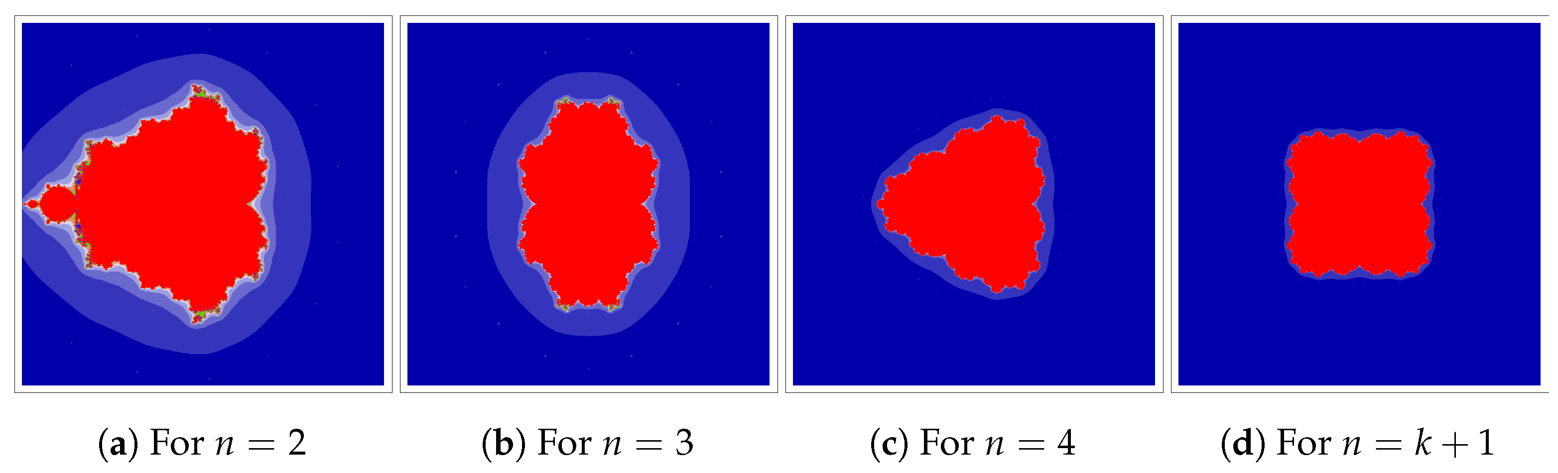
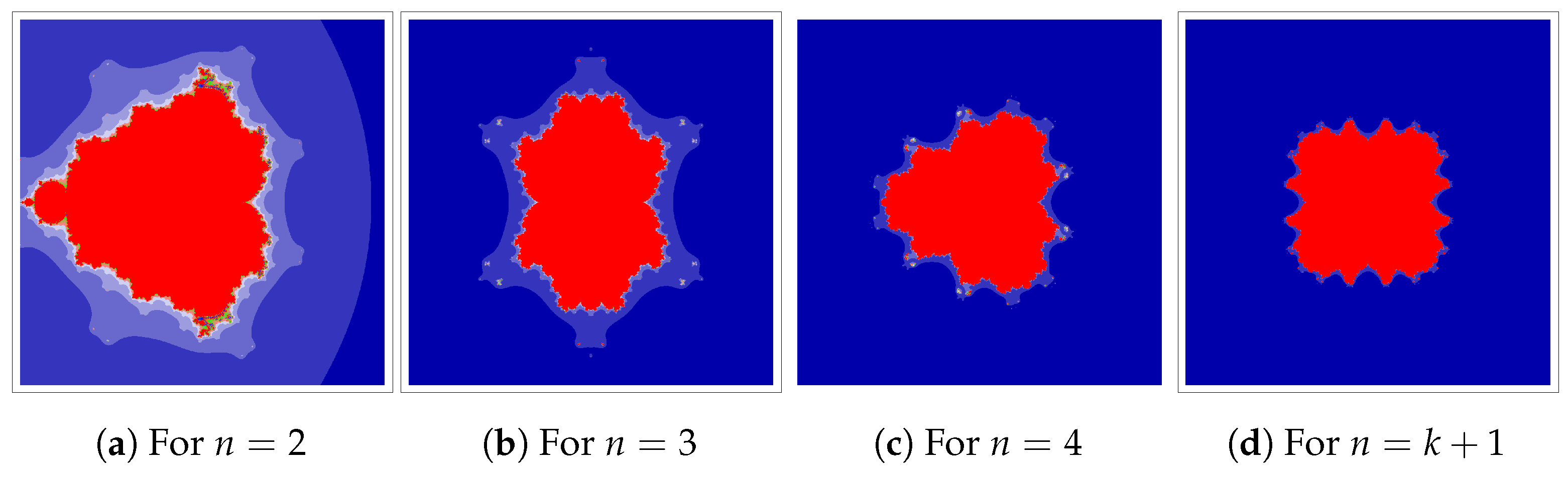
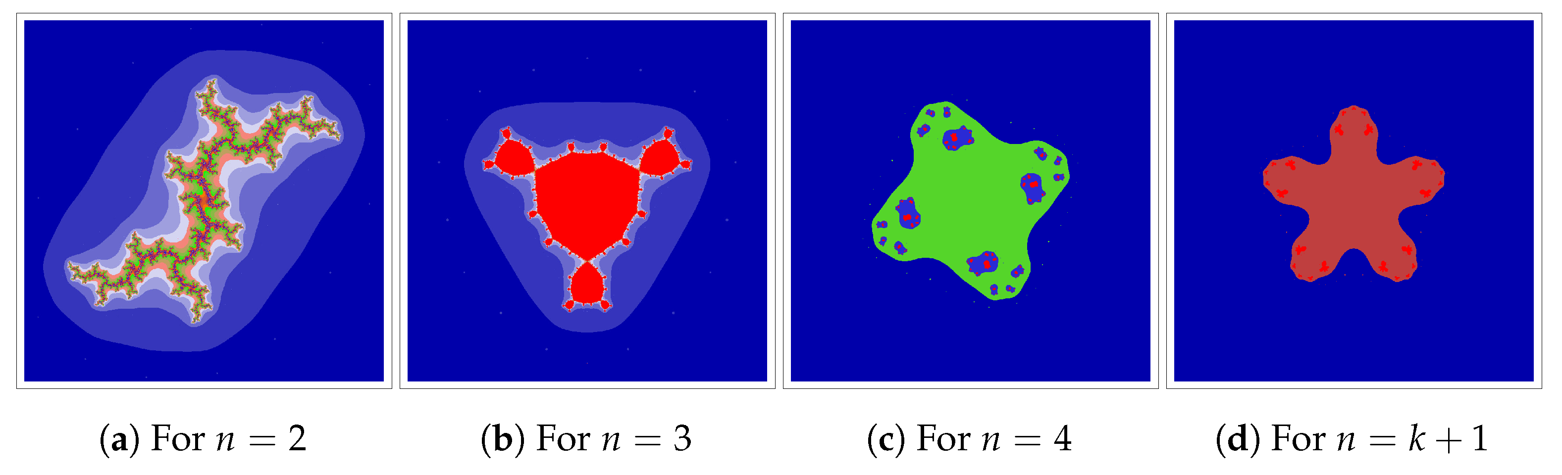
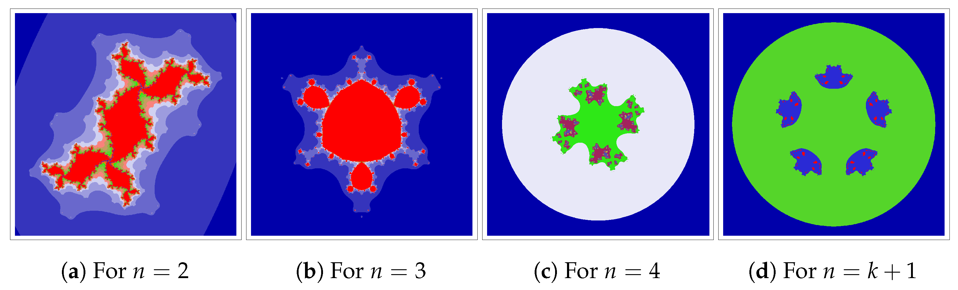
We start with an example outlining how the Jungck–DK iteration can be used. We will use ${\mathcal{Q}}_c\left(z\right)=z^{p+1}+1.5z+c,$ at $p=1,2,3$ and 4. In Figure 2, Figure 3, Figure 4 and Figure 5, we fix $A={[-2.5,2.5]}^2$ and change the parameters $\rho$ and $\varrho$ of iteration. We can observe that varying $\rho$ and $\varrho$ values in the Jungck–DK method has a substantial effect on the shape of the resulting set.

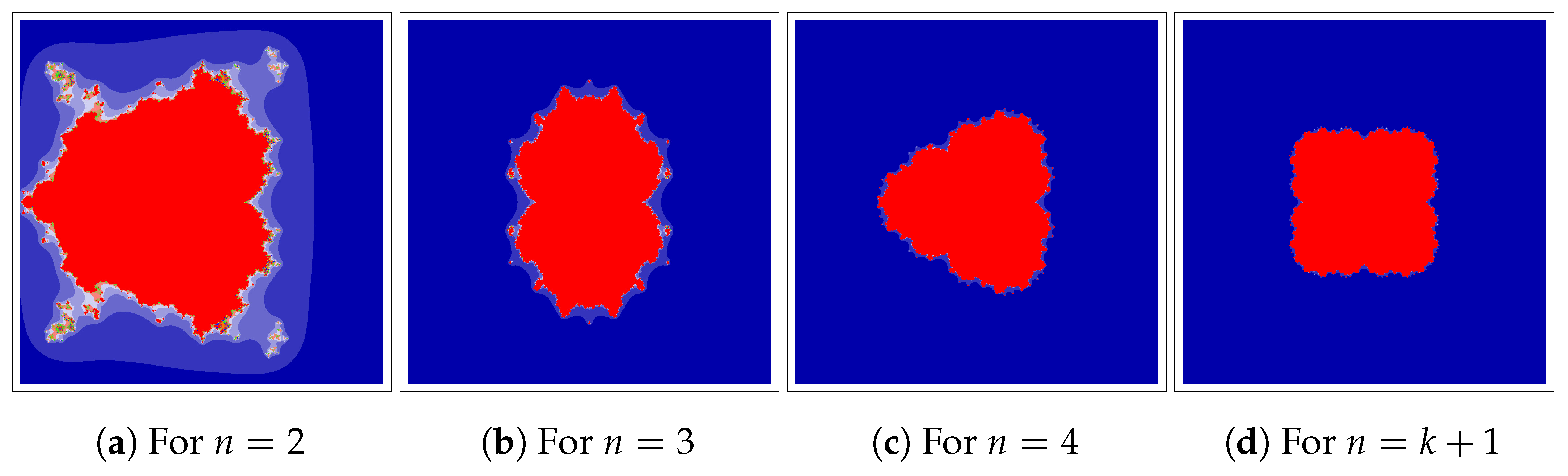
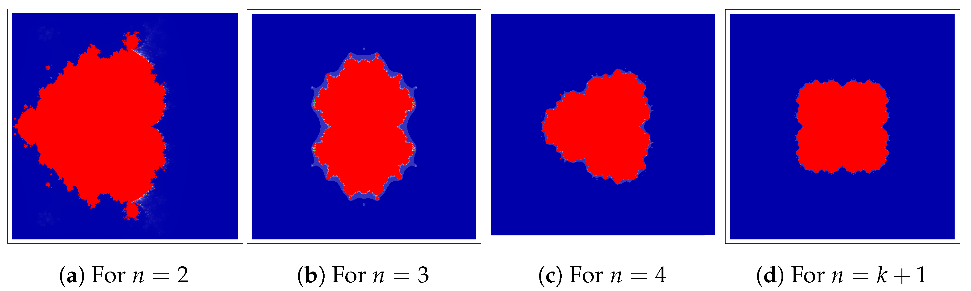
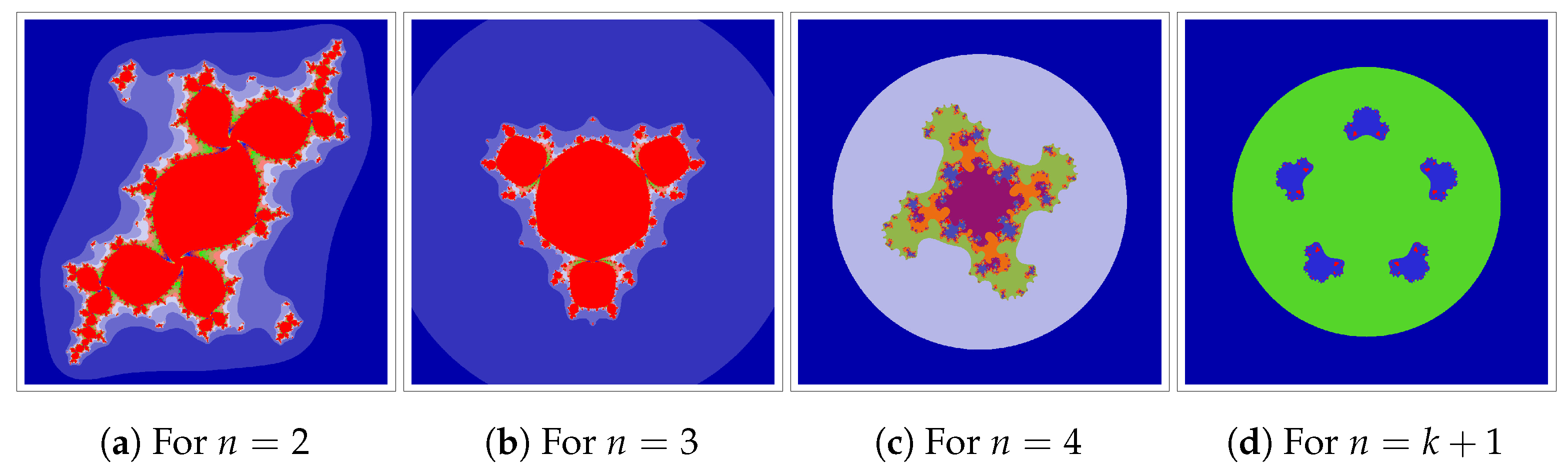
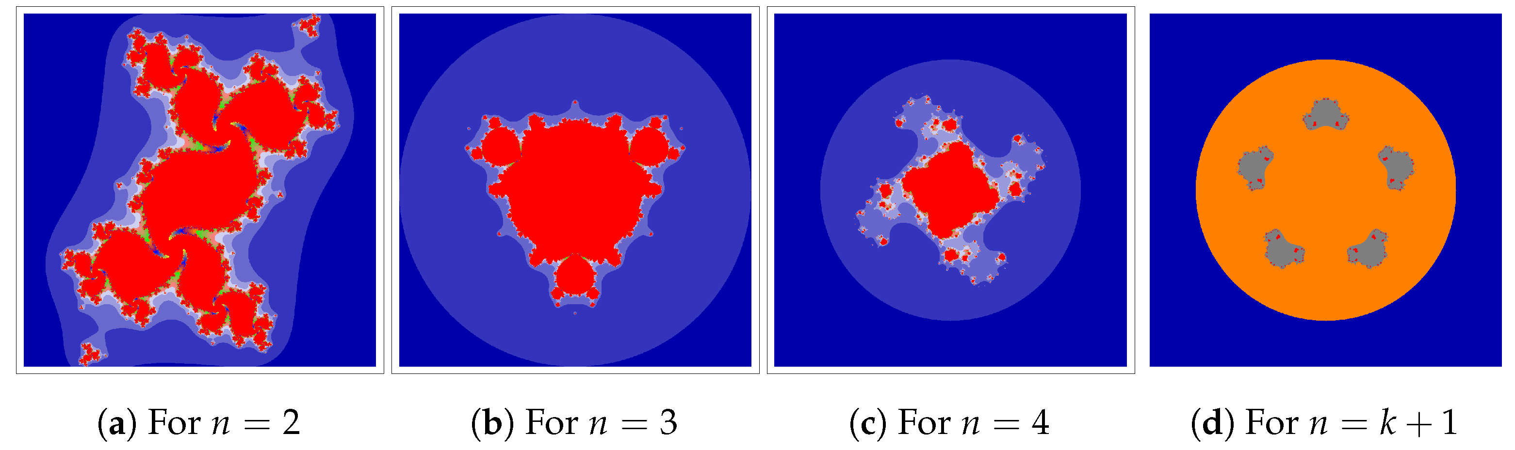
4.1.2. Examples of Julia Sets in Jungck–DK Orbit

In the following example, a Julia set for ${\mathcal{Q}}_c\left(z\right)=z^{p+1}+1.5z+c,$ at $p=1,2,3$ and 4, is generated using the Jungck–DK iteration. The images were obtained for $A={[-2.5,2.5]}^2$ and $c=1.85i$ and for different parameters $\rho$ and $\varrho .$ Changing the parameters of the Jungck–DK iteration allows us to obtain different Julia set shapes, as shown in Figure 6, Figure 7, Figure 8 and Figure 9, for the same generating polynomial.

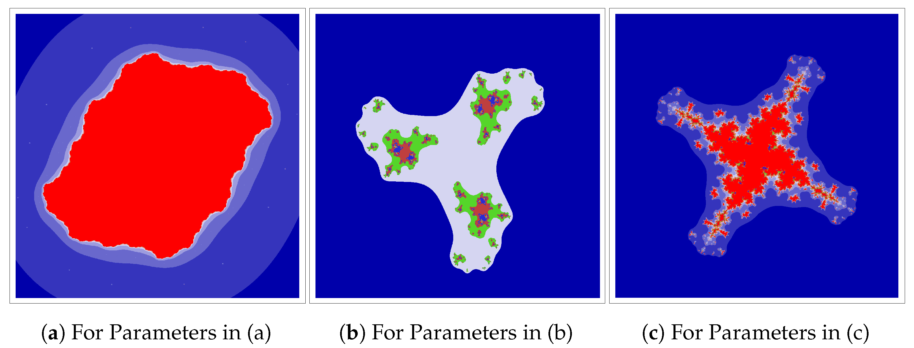
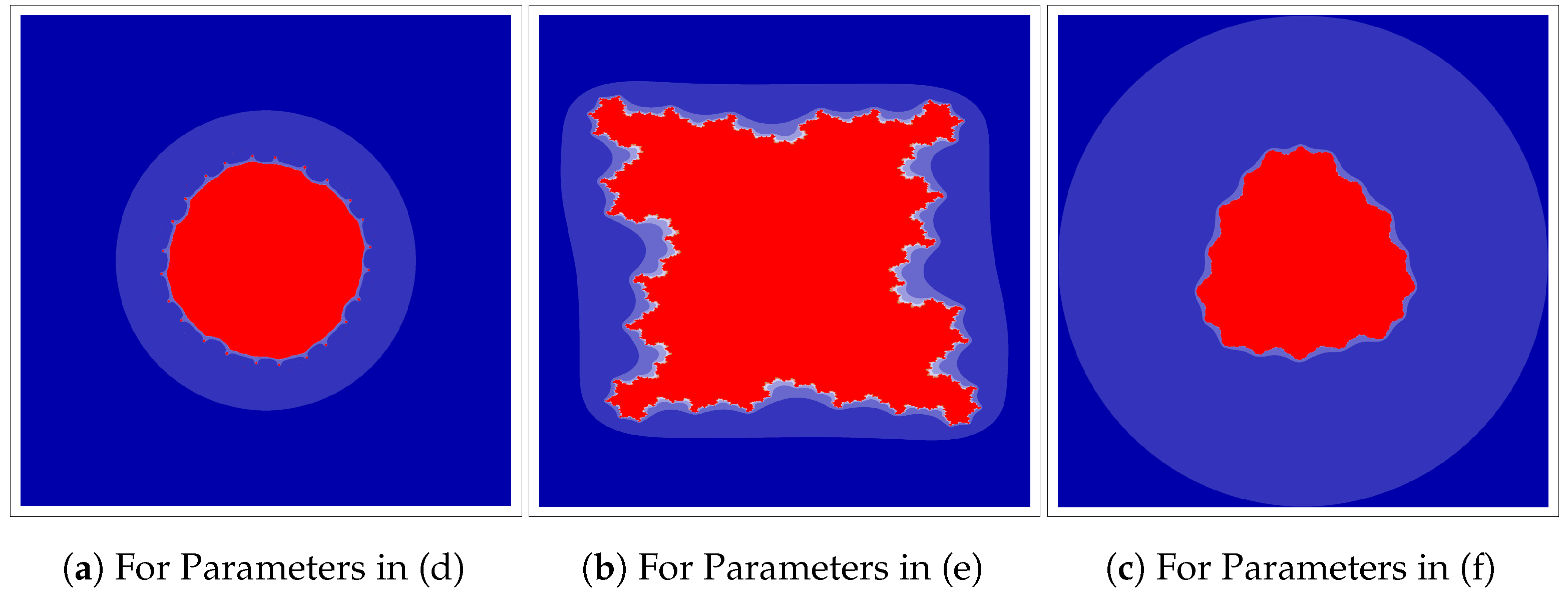
In the second example, various Julia sets generated using the Jungck–DK iteration are presented. The following parameters were utilised in order to generate the images of Julia sets shown in Figure 10 and Figure 11.

(a)

${\mathcal{Q}}_c\left(z\right)=z^2+2.32z+c,$$c=1.85i$, $A=[-3.5,3.5]\times [-3.2,3.2]$, a Jungck–DK iteration with $\rho =0.2=\varrho .$

(b)

${\mathcal{Q}}_c\left(z\right)=z^3+3.167z+c,$$c=5+6.3i$, $A=[-3.1,3.1]\times [-3.5,3.5]$, a Jungck–DK iteration with $\rho =0.5=\varrho .$

(c)

${\mathcal{Q}}_c\left(z\right)=z^4+3.75z+c,$$c=3.9-7i$, $A={[-2.5,2.5]}^2$, a Jungck–DK iteration with $\rho =0.6=\varrho .$

(d)

${\mathcal{Q}}_c\left(z\right)=z^5+5.25z+c,$$c=-0.5+7i$, $A={[-4.5,4.5]}^2$, a Jungck–DK iteration with $\rho =0.3=\varrho .$

(e)

${\mathcal{Q}}_c\left(z\right)=z^2+4.123z+c,$$c=5.2-3.1i$, $A=[-8.5,8.5]\times [-5.5,5.5]$, a Jungck–DK iteration with $\rho =0.3,\varrho =0.7.$

(f)

${\mathcal{Q}}_c\left(z\right)=z^3+6.80z+c,$$c=-2.2-6.1$, $A={[-6.5,6.5]}^2$, a Jungck–DK iteration with $\rho =0.4,\varrho =0.9.$

Using various combinations of the parameters, such as polynomials, Jungck–DK iteration parameters, etc., we are able to generate artistically applicable fractal patterns with a great deal of diversity.

5. Conclusions

In this paper, we propose and analyze the Jungck–DK iterative scheme for approximating fixed points. Our main contributions are summarized as follows. Firstly, we demonstrate the stability and faster convergence of the Jungck–DK iterative scheme compared to other Jungck-type schemes, such as the Jungck–CR, Jungck–SP, and Jungck–S schemes. Secondly, we provide a numerical example to illustrate the rate of convergence and prove the data dependence result for the Jungck–DK iterative scheme. Lastly, we apply the Jungck–DK iterative scheme to calculate the escape criteria of polynomial functions, generating distinct images of the Mandelbrot and Julia sets.

Therefore, these fractals have become useful in diverse scientific and engineering applications. Through our analysis of Julia sets, we have found that the size of the explored fractals is dependent on the parameters $\rho$ and $\varrho$, while the shape and symmetry are influenced by the parameters a and c. Furthermore, as we increase the value of n, the area occupied by the fractals decreases.

Concerning new directions of research, Nandal et al. [35] developed a generalized viscosity approximation method in the context of a Hilbert space, which was applied to a range of problems, such as variational inequalities, convex feasibility problems, and fixed-point problems. These applications demonstrated the versatility and usefulness of the proposed iterative method in fixed-point theory. Building on this, it will be very interesting to explore the potential of this method in generating fractals, particularly Julia and Mandelbrot sets. Moreover, using our iterative method, a new type of viscosity approximation method can be found, which can be used as an effective tool for generating fractals with complex structures.

References

1. Abbas, M.; Jungck, G. Common fixed point results for noncommuting mappings without continuity in cone metric spaces. J. Math. Anal. Appl. 2008, 341, 416–420. [Google Scholar] [CrossRef]
2. Bouhadjera, H. A unique common fixed point for contractive mappings under a new concept. In Bulletin of the Transilvania University of Brasov; Series III: Mathematics and Computer Science; Transilvania University Press: Brasov, Romania, 2022; pp. 33–46. [Google Scholar]
3. Kumar, S.; Aron, D. Common fixed-point theorems for non-linear non-self contractive mappings in convex metric spaces. Topol. Algebra Its Appl. 2023, 11, 20220122. [Google Scholar] [CrossRef]
4. Chandok, S.; Radenović, S. Existence of solution for orthogonal F-contraction mappings via Picard–Jungck sequences. J. Anal. 2022, 30, 677–690. [Google Scholar] [CrossRef]
5. Fan, H.; Wang, C. Stability and convergence rate of Jungck-type iterations for a pair of strongly demicontractive mappings in Hilbert spaces. Comput. Appl. Math. 2023, 14, 33. [Google Scholar] [CrossRef]
6. Maldar, S. An examination of data dependence for Jungck-Type iteration method. Erciyes Üniv. Fen Bilim. Enstitüsü Fen Bilim. Derg. 2020, 36, 374–384. [Google Scholar]
7. Jamil, Z.Z.; Hussein, Z. Common Fixed Point of Jungck Picard Itrative for Two Weakly Compatible Self-Mappings. Iraqi J. Sci. 2021, 62, 1695–1701. [Google Scholar]
8. Bosede, A.O. Strong convergence results for the Jungck-Ishikawa and Jungck-Mann iteration processes. Bull. Math. Anal. Appl. 2010, 2, 65–73. [Google Scholar]
9. Chugh, R.; Kumar, V. Strong Convergence and Stability results for Jungck-SP iterative scheme. Int. J. Comput. Appl. 2011, 36, 40–46. [Google Scholar]
10. Hussain, N.; Kumar, V.; Kutbi, M.A. On rate of convergence of Jungck-type iterative schemes. Abstr. Appl. Anal. 2013, 2013, 132626. [Google Scholar] [CrossRef]
11. Berinde, V. On the convergence of the Ishikawa iteration in the class of quasi contractive operators. Acta Math. Univ. Comen. New Ser. 2004, 73, 119–126. [Google Scholar]
12. Singh, S.L.; Bhatnagar, C.; Mishra, S.N. Stability of Jungck-type iterative procedures. Int. J. Math. Math. Sci. 2005, 19, 3035–3043. [Google Scholar] [CrossRef]
13. Ostrowski, A.M. The Round-off Stability of Iterations. ZAMM-J. Appl. Math. Mech./Z. Angew. Math. Mech. 1967, 47, 77–81. [Google Scholar] [CrossRef]
14. Harder, A.M. Fixed Point Theory and Stability Results for Fixed Point Iteration Process. Ph.D.Thesis, University of Missouri-Rolla, Rolla, MO, USA, 1987. [Google Scholar]
15. Jungck, G. Commuting mappings and fixed points. Am. Math. Mon. 1976, 83, 261–263. [Google Scholar] [CrossRef]
16. Olatinwo, M.O.; Imoru, C.O. Some convergence results for the Jungck–Mann and the Jungck–Ishikawa iteration processes in the class of generalized Zamfirescu operators. Acta Math. Univ. Comen. New Ser. 2008, 27, 299–304. [Google Scholar]
17. Olatinwo, M.O. A generalization of some convergence results using the Jungck-Noor three step iteration process in arbitrary Banach space. Fasc. Math. 2008, 40, 37–43. [Google Scholar]
18. Qing, Y.; Rhoades, B.E. Comments on the rate of convergence between Mann and Ishikawa iterations applied to Zamfirescu operators. Fixed Point Theory Appl. 2008, 2018, 387504. [Google Scholar] [CrossRef]
19. Jungck, G.; Hussain, N. Compatible maps and invariant approximations. J. Math. Anal. Appl. 2007, 325, 1003–1012. [Google Scholar] [CrossRef]
20. Osilike, M.O.; Udomene, A. Short proofs of stability results for fixed point iteration procedures for a class of contractive-type mappings. Indian J. Pure Appl. Math. 1999, 30, 1229–1234. [Google Scholar]
21. Berinde, V.; Takens, F. Iterative Approximation of Fixed Points; Springer: Berlin/Heidelberg, Germany, 2007; Volume 1912. [Google Scholar]
22. Şoltuz, Ş.M.; Grosan, T. Data dependence for Ishikawa iteration when dealing with contractive-like operators. Fixed Point Theory Appl. 2008, 2008, 242916. [Google Scholar] [CrossRef]
23. Shirriff, K. Fractals from simple polynomial composite functions. Comput. Graph. 1993, 17, 701–703. [Google Scholar] [CrossRef]
24. Mandelbrot, B.B. The Fractal Geometry of Nature; WH Freeman: New York, NY, USA, 1982. [Google Scholar]
25. Fatou, P. Sur les équations fonctionnelles. Bull. Soc. Math. Fr. 1919, 47, 161–271. [Google Scholar] [CrossRef]
26. Julia, G. Mémoire sur l’itération des fonctions rationnelles. J. Math. Pures Appl. 1918, 8, 47–245. [Google Scholar]
27. Antal, S.; Tomar, A.; Prajapati, D.J.; Sajid, M. Fractals as Julia sets of complex sine function via fixed point iterations. Fractal Fract. 2021, 5, 272. [Google Scholar] [CrossRef]
28. Tomar, A.; Kumar, V.; Rana, U.S.; Sajid, M. Fractals as Julia and Mandelbrot Sets of Complex Cosine Functions via Fixed Point Iterations. Symmetry 2023, 15, 478. [Google Scholar] [CrossRef]
29. Dhurandhar, S.V.; Bhavsar, V.C.; Gujar, U.G. Analysis of z-plane fractal images from z+ c for α<0. Comput. Graph. 1993, 17, 89–94. [Google Scholar]
30. Gdawiec, K. Fractal patterns from the dynamics of combined polynomial root finding methods. Nonlinear Dyn. 2017, 90, 2457–2479. [Google Scholar] [CrossRef]
31. Hamada, N.; Kharbat, F. Mandelbrot and Julia Sets of Complex Polynomials Involving Sine and Cosine Functions via Picard–Mann Orbit. Complex Anal. Oper. Theory 2023, 17, 13. [Google Scholar] [CrossRef]
32. Shahid, A.A.; Nazeer, W.; Gdawiec, K. The Picard–Mann iteration with s-convexity in the generation of Mandelbrot and Julia sets. Monatshefte Math. 2021, 195, 565–584. [Google Scholar] [CrossRef]
33. Antal, S.; Tomar, A.; Prajapati, D.J.; Sajid, M. Variants of Julia and Mandelbrot sets as fractals via Jungck-Ishikawa fixed point iteration system with s-convexity. AIMS Math. 2022, 7, 10939–10957. [Google Scholar] [CrossRef]
34. Tanveer, M.; Nazeer, W.; Gdawiec, K. On the Mandelbrot set of zp+ logct via the Mann and Picard–Mann iterations. Math. Comput. Simul. 2023, 209, 184–204. [Google Scholar] [CrossRef]
35. Nandal, A.; Chugh, R.; Postolache, M. Iteration process for fixed point problems and zeros of maximal monotone operators. Symmetry 2019, 11, 655. [Google Scholar] [CrossRef]
Figure 1. Convergence behaviour of Jungck-type iterative schemes.
Fractalfract 07 00418 g001
Figure 2. Mandelbrot sets for the parameters ρ = 0.01 and ϱ = 0.2 .
Fractalfract 07 00418 g002
Figure 3. Mandelbrot sets for the parameters ρ = 0.3 and ϱ = 0.6 .
Fractalfract 07 00418 g003
Figure 4. Mandelbrot sets for the parameters ρ = 0.5 and ϱ = 0.4 .
Fractalfract 07 00418 g004
Figure 5. Mandelbrot sets for the parameters ρ = 0.9 and ϱ = 0.09 .
Fractalfract 07 00418 g005
Figure 6. Julia sets for the parameters ρ = 0.01 and ϱ = 0.2 .
Fractalfract 07 00418 g006
Figure 7. Julia sets for the parameters ρ = 0.3 and ϱ = 0.6 .
Fractalfract 07 00418 g007
Figure 8. Julia sets for the parameters ρ = 0.5 and ϱ = 0.4 .
Fractalfract 07 00418 g008
Figure 9. Julia sets for the parameters ρ = 0.9 and ϱ = 0.09 .
Fractalfract 07 00418 g009
Figure 10. Julia sets for different parameters, e.g., polynomials, area, and values of c, ρ , and ϱ .
Fractalfract 07 00418 g010
Figure 11. Julia sets for different parameters, e.g., polynomials, area, and values of c, ρ , and ϱ .
Fractalfract 07 00418 g011