Stability Criteria and Λ-Fractional Mechanics

Abstract

Global stability criteria for Λ-fractional Mechanics are established. The fractional extension of a bar under axial loading is discussed. Globally minimizing the total energy function, non-smooth deformations are introduced. The co-existence of phases phenomenon is established in Λ-fractional elasticity. It is pointed out that global minimization only is valid in fractional analysis.

1. Introduction

Fractional derivative models have been introduced to describe the deformation of various models in mechanics. Bagley et al. [1,2] introduced fractional viscoelastic models, trying to simulate their experiments. Atanackovic [3] has presented a series of papers establishing the fractional deformation of the materials. Mainardi [4] has presented wave propagation in viscoelastic materials with fractional calculus. Lazopoulos [5], turning the interest from time to space, just to discuss non-homogeneous materials with possible voids, etc., proposed a model with fractional space derivatives. Noll’s axiom of local action, Truesdell [6], is not valid anymore. Hence, the stress at a point does not depend only upon the (local) strain at that point, but on the strain of a region around the point. That postulate was introduced by Eringen [7], indicating that in micro and nano materials the stress at a point depends on the deformation of a region around that point, contrary to the conventional elasticity based upon Noll’s axiom.

Leibniz [8] originated fractional calculus, with Liouville [9], Riemann [10], and other famous mathematicians, which has recently been applied to modern engineering advances, mechanics, physics, biology, bioengineering, etc., introducing non-local derivatives. The theory and applications of fractional calculus, in many physical areas, may also be found in various books. Samko et al. [11] has been one of the most reliable sources of information concerning fractional calculus. Poldubny [12] is a classic book concerning fractional differential equations. Oldham et al. [13] is one of the first texts in that area and Miller et al. [14] is a text with information on both theory and fractional differential equations.

It is evident that fractional derivatives not only abolish the local character of the conventional derivatives but also fail to be derivatives satisfying the prerequisites of Differential Topology, Chillingworth [15], which are:

• Linearity $D\left(af\left(x\right)+bg\left(x\right)\right)=aDf\left(x\right)+bDg\left(x\right)$.
• Leibniz rule $D\left(f\left(x\right)·g\left(x\right)\right)=Df\left(x\right)·g\left(x\right)+f\left(x\right) Dg\left(x\right).$
• Chain rule $D\left(g\left(f\right)\right)\left(x\right)=Dg(f\left(x\right)·Df\left(x\right)$.

Since the use of fractional calculus in physics, mechanics, engineering, biology, economics, etc., is questionable, Lazopoulos [16] has tried to fill that gap, proposing Λ-fractional analysis with the Λ-fractional derivative, satisfying all the necessary postulates of differential topology for real mathematical derivatives. Λ-fractional analysis was applied to mechanics, differential equations, geometry, physics, etc., in Lazopoulos [17,18,19,20]. However, although Λ-fractional analysis responds to the need for global considerations of a problem, what has been overlooked is the global stability analysis of those problems. Indeed, the considered stability analysis is local, whereas all the other factors of the problems are global. That defect is pointed out and corrected in the present work, invoking global stability criteria, contrary to the well-known local used in similar procedures. Discontinuities introduced by Weierstrass–Erdman conditions may be considered and globally stable states may be examined. Only the co-existence of phases phenomena, introduced by Ericksen in [21], will be recognized in the present case. Nevertheless, in Λ-fractional analysis, there is not any possibility of the consideration of locally stable conditions. Globally, stable states with corner conditions, per Fomin et al. [22], are the mathematically correct configurations.

Just to show the applicability of the proposed ideas, the Λ- fractional deformation of a bar under axial tension is discussed, transferring the ideas of globally stable states into the present Λ-fractional analysis. It should be pointed out that the present analysis is imperative in Λ-fractional analysis, contrary to the conventional one, which is optional, where local criteria may also be allowed, following the adapted stability convention.

In the following sections, Λ-fractional analysis is outlined and is applied upon the deformation of an axially loaded bar. The initial and the corresponding Λ-fractional spaces are defined. The axial deformation of the bar is studied in the Λ-fractional space, adopting the conventional deformation theory. However, only globally stable states of the bar are allowed. The deformed placement of the bar in the initial space is defined, transferring the deformation from the Λ-space into the initial space. The present work may serve as a model for considering further mathematical and physical problems in the context of Λ-fractional analysis.

2. Fractional Calculus

A recent important branch of applied mathematics is fractional calculus. Its main characteristic is global analysis. Leibnitz [8] suggested fractional derivatives after establishing the local derivatives he had already introduced. Various branches of applied science, such as physics, mechanics, biology, economy, etc., have introduced fractional calculus in their analytical procedures for a better description of various globally dependent phenomena. Lately, many books [10,11,12,13] include information regarding fractional calculus, which is, in fact, a global mathematical analysis.

The fractional integrals are defined by:

$${}_{a}I_x^{\gamma }f(x)=\frac{1}{\mathrm{\Gamma }(\gamma )}{\displaystyle \underset{a}{\overset{x}{\int }}\frac{f(s)}{{(x-s)}^{1-\gamma }}ds}$$

(1)

$${}_{x}I_b^{\gamma }f(x)=\frac{1}{\mathrm{\Gamma }(\gamma )}{\displaystyle \underset{x}{\overset{b}{\int }}\frac{f(s)}{{(s-x)}^{1-\gamma }}ds}$$

(2)

for a fractional dimension 0 < γ $\le$ 1. Equation (1) defines the left and Equation (2) the right fractional integral, whereas γ is the order of fractional integrals and Γ(γ) is Euler’s Gamma function. Although many fractional derivatives exist, the Riemann–Liouville fractional derivative (R-L) will be considered, defined by:

$${}_a{}^{RL}D{}_x^{\gamma }f(x)=\frac{d}{dx}\left({}_{a}I_x^{1-\gamma }\left(f(x)\right)\right)=\frac{1}{\mathrm{\Gamma }(1-\gamma )}\frac{d}{dx}{\displaystyle \underset{a}{\overset{x}{\int }}\frac{f(s)}{{(x-s)}^{\gamma }}ds}.\hspace{1em}$$

(3)

That is the left R-L derivative, whereas the right Riemann–Liouville’s fractional derivative (R-L) is defined by:

$${}_x{}^{RL}Df(x)=\frac{d}{dx}\left({}_{x}I_b^{1-\gamma }\left(f(x)\right)\right)=-\frac{1}{\mathrm{\Gamma }(1-\gamma )}\frac{d}{dx}{\displaystyle \underset{x}{\overset{b}{\int }}\frac{f(s)}{{(s-x)}^{\gamma }}ds}.$$

(4)

The fractional integrals and derivatives are related by the expression

$${}_a{}^{RL}D{}_x^{\gamma }\left({}_a{}^{}{\rm I}{}_x^{\gamma }f\left(x\right)\right)=f\left(x\right)$$

(5)

Since fractional calculus, based upon fractional derivatives, is not sufficient to generate differentials, Lazopoulos [16] proposed Λ-fractional analysis, just to bridge the inability of fractional derivatives to generate differentials. Consequently, important mathematical tools used in many scientific applications, such as calculus of variations, differential geometry, field theorems, existence and uniqueness theorems of differential equations, etc., may not work in fractional calculus. However, some researchers have proposed fractional differentials, fractional variational procedures, fractional differential geometries, fractional field theories, etc., although their mathematical accuracy is under question. The Λ-fractional analysis proposes a dual space, the Λ-fractional space, where everything behaves conventionally. Therefore, the derivatives in the proposed Λ-space are local and differentials may be generated. Further differential geometry is established with variational procedures and field theorems. In addition, Λ-fractional analysis can generate theorems corresponding to the existence and uniqueness of the fractional differential equations. The Λ-fractional derivative (Λ-FD) is defined by:

$${}_a{}^{\Lambda }D{}_x^{\gamma }f(x)=\frac{{}_{\alpha }{}^{RL}D{}_x^{\gamma }f(x)}{{}_a{}^{RL}D{}_x^{\gamma }x}$$

(6)

Recalling Equation (3), the Λ-FD is defined by

$${}_a{}^{\Lambda }D{}_x^{\gamma }f\left(x\right)=\frac{\frac{d{}_{a}I_x^{1-\gamma }f(x)}{dx}}{\frac{d{}_{a}I_x^{1-\gamma }x}{dx}}=\frac{d_a{I}_x{}^{1-\gamma }f(x)}{d_a{I}_x{}^{1-\gamma }x}$$

(7)

The dual Λ-fractional space to the initial space is defined by (X, F(X)) coordinates, with

$$X{=}_a{I}_x{}^{1-\gamma }x,\hspace{1em}\hspace{1em}F(X){=}_a{I}_x{}^{1-\gamma }f(x(X))$$

(8)

Thus, the Λ-FD is a local derivative in the dual, Gao [22], Λ-fractional space (X, F(X)). Hence, conventional mathematical analysis applied in that space acquires the demanded accuracy. Consequently, differential geometry exists in that dual space. Further, no question arises concerning the accuracy of various other important mathematical tools used in applications, such as variational procedures and field theorems, existence and uniqueness theorems of differential equations. Further, the various results may be transferred into the initial space, that is, the dual to the dual, Gao [22], of the initial space, following the relation

$$f\left(x\right)={}_a{}^{RL}D{{}_x^{1-\gamma }}^{}F\left(X\left(x\right)\right)={}_{\alpha }{}^{RL}D{{}_x^{1-\gamma }}^{}{}_a{}^{}I{}_x^{1-\gamma }f\left(x\right)$$

(9)

3. Globally Stable Λ-Fractional Bars

A bar in the initial space is defined in its undeformed placement (placement at ease, Truesdell [6]) by

$$x \epsilon L=[0, 1]\hspace{1em}0<L<\infty .$$

(10)

The deformed (current) placement in the initial space after the application of the axial force p at the end x = L of the bar is defined by y(x), with

$$y\left(x\right)=x+u\left(x\right),$$

(11)

where u(x) is the displacement field due to the action of the axial load p. Further, the constant cross-section bar area α is considered.

Transferring the problem into the (dual) Λ-fractional space, the corresponding parameters of the problem (X, U(X), Y(X), P) are defined through

$$X=\frac{1}{\mathit{\Gamma }\left(1-\gamma \right)}{{\displaystyle \int }}_0^x\frac{x}{{\left(x-s\right)}^{\gamma }}ds=\frac{x^{2-\gamma }}{\mathit{\Gamma }\left(3-\gamma \right),}$$

(12)

and

$$x={\left(X\mathit{\Gamma }\left(3-\gamma \right)\right)}^{1/\left(2-\gamma \right)}$$

(13)

Further,

$$U\left(x\right)=\frac{1}{\mathit{\Gamma }\left(1-\gamma \right)}{{\displaystyle \int }}_0^x\frac{u\left(s\right)}{{\left(x-s\right)}^{\gamma }}ds$$

(14)

Introducing, moreover, the value of x into Equation (14), the displacement U(X) is defined.

The total energy of the bar in the Λ-space is expressed by

$$V\left(X\right)={{\displaystyle \int }}_0^L\left(\mathrm{W}\left(\frac{dU\left(X\right)}{dX}\right)-P\frac{dU\left(X\right)}{dX}\right)dX={{\displaystyle \int }}_0^{L}F\left(X,U\left(X\right),U^{\prime }\left(X\right)\right)dX$$

(15)

The equilibrium equation is defined by the minimum of the total energy V(X), expressed by

$$\frac{d}{dX}\frac{\partial \mathrm{W}\left(U^{\prime }\left(X\right)\right)}{\partial \mathrm{U} \prime \left(\mathrm{X}\right)}=0,$$

(16)

with the boundary conditions U(0) = 0 and

$$P=\frac{\partial W\left(U^{\prime }\left(L\right)\right)}{\partial U^{\prime }\left(L\right)} \mathrm{or} U\left(L\right) = B.$$

(17)

In conventional equilibrium problems, one has to solve the above equilibrium problem just to complete the solution. That is valid because the local criterion of stability is adopted. However, when global stability criteria are considered, the coexistence of phases phenomenon appears due to the non-local criterion of stability.

Globally stable equilibrium states have been introduced by Ericksen [21], describing the co-existence of mixed states with low and high-strain states. Those states are similar to the co-existing phases of melting ice, with the coexistence of ice and water. James [23] also describes the co-existence of phases phenomenon in solids, following Ericksen’s model. In the latter equilibrium placements, jumping of the strains is accepted. Since everything concerning fractional calculus is global, only global criteria should be considered, in the present Λ-fractional analysis.

It should be pointed out that only globally stable variational procedures are allowed in fractional calculus problems. The Weierstrass–Erdman corner conditions [24] should additionally be satisfied with

$$F_{U’}[x=c-0]-F_{U’}[x=c+0]=0$$

(18)

$$(F-U’F_{U’})[x=c-0]-(F-U’F_{U’})[x=c+0]=0.$$

(19)

It is necessary to fulfil those conditions for any fractional equilibrium problem.

The diagram of the stresses in the Λ-space is shown in Figure 1.

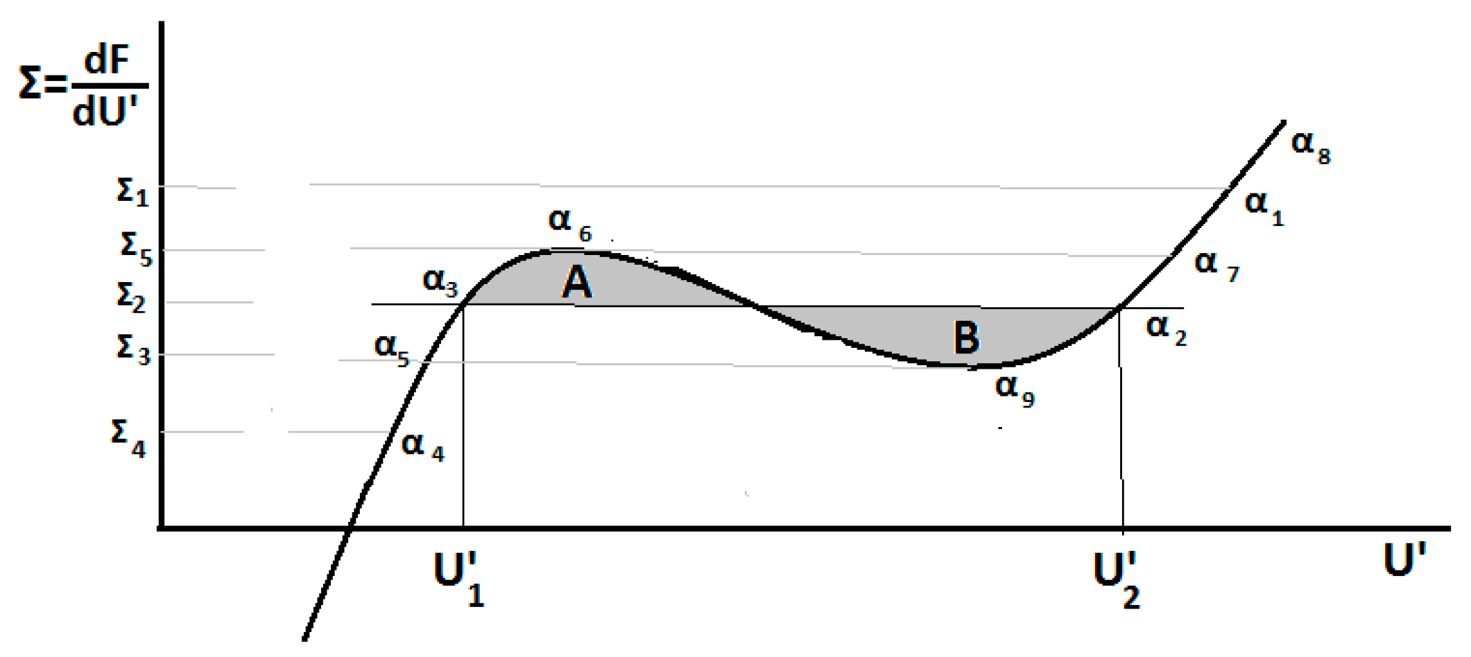
Just to understand the difference between the locally and globally stable criteria, the diagram of the stress Σ versus the strain U$’$ of the bar in the Λ-space is shown in Figure 2.

The strains of the bar, in Figure 2, are always very high around the pole of the fractional analysis (x = 0). Therefore, the discussion starts out the point α_1, corresponding to the stress Σ₁. Discussing first the locally stable states, the path α₁ − α₉ should be followed. A minimum of the stress Σ exists at the point α₉. Hence, jumping to point α₅ takes place. Reducing the stress, the following path is described by the path of the strains α₃ − α_4. Increasing the strains, the path α₄ − α₅ − α₃ − α₆ is followed. Increasing the stress more, jumping to strain α₇ takes place, and by increasing the strain field the path α₇ − α₈ is followed. Consequently, a loss of energy appears, following the cycle α₅ − α₆ − α₇ − α₉ − α₅.

Proceeding to the discussion of the global stability analysis, exhibiting the coexistence of phases phenomenon, the path of strains α₁ − α₂ is followed. The strains α₂, α₃ define the coexisting strains satisfying the Weierstrass–Erdman conditions. In that case, the equality of areas A and B is valid. A reduction in the stresses of the path α₃ − α₄ follows. Increasing the stresses of the path of strains α₄ − α₅ − α₃ − α₆ − α₇ − α₈ is considered. For the fractional problems that are inherently global, only global stability criteria with the coexisting states should be involved. Hence, in fractional variational procedures, the accepted minimum paths should satisfy the Weierstrass–Erdman corner conditions.

4. Application

Consider a bar of length L = 1 and cross-section area A in the initial space. The left end of the bar is fixed and an axial force equal to P is applied at the other. Therefore, the bar with 0 < x < 1 in the initial space is transferred in the dual Λ-fractional space with fractional order γ = 0.6. Hence, the bar in the Λ-space is defined with

$$X=\frac{1}{\mathrm{\Gamma }\left(0.4\right)}{{\displaystyle \int }}_0^x\frac{x}{{\left(x-s\right)}^{0.6}}ds=\frac{x^{1.4}}{\mathit{\Gamma }\left(2.4\right)}=0.805x^{1.4}$$

(20)

Therefore, the length of the rod in the dual Λ-space is L^Λ = 0.805.

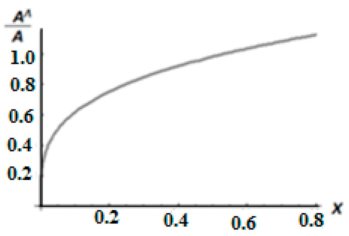
The constant cross-section area A of the bar in the initial space becomes, in the dual Λ-space, A^Λ, with

$$A^{\Lambda }=\frac{A{x}^{1-\gamma }}{\mathit{\Gamma }\left(2-\gamma \right)}=\frac{A{\left({\rm X}\mathit{\Gamma }\left(3-\gamma \right)\right)}^{\frac{1-\gamma }{2-\gamma }}}{\mathit{\Gamma }\left(2-\gamma \right)}=1.199A{{\rm X}}^{0.29}$$

(21)

Figure 3 is the diagram of the ratio of the cross-sections A^Λ/A in the Λ-space and the initial one.

The force p applied at the end of the bar becomes P in the Λ-space, with

$$P=\frac{p{L}^{1-\gamma }}{\mathit{\Gamma }\left(2-\gamma \right)}=1.1270p$$

(22)

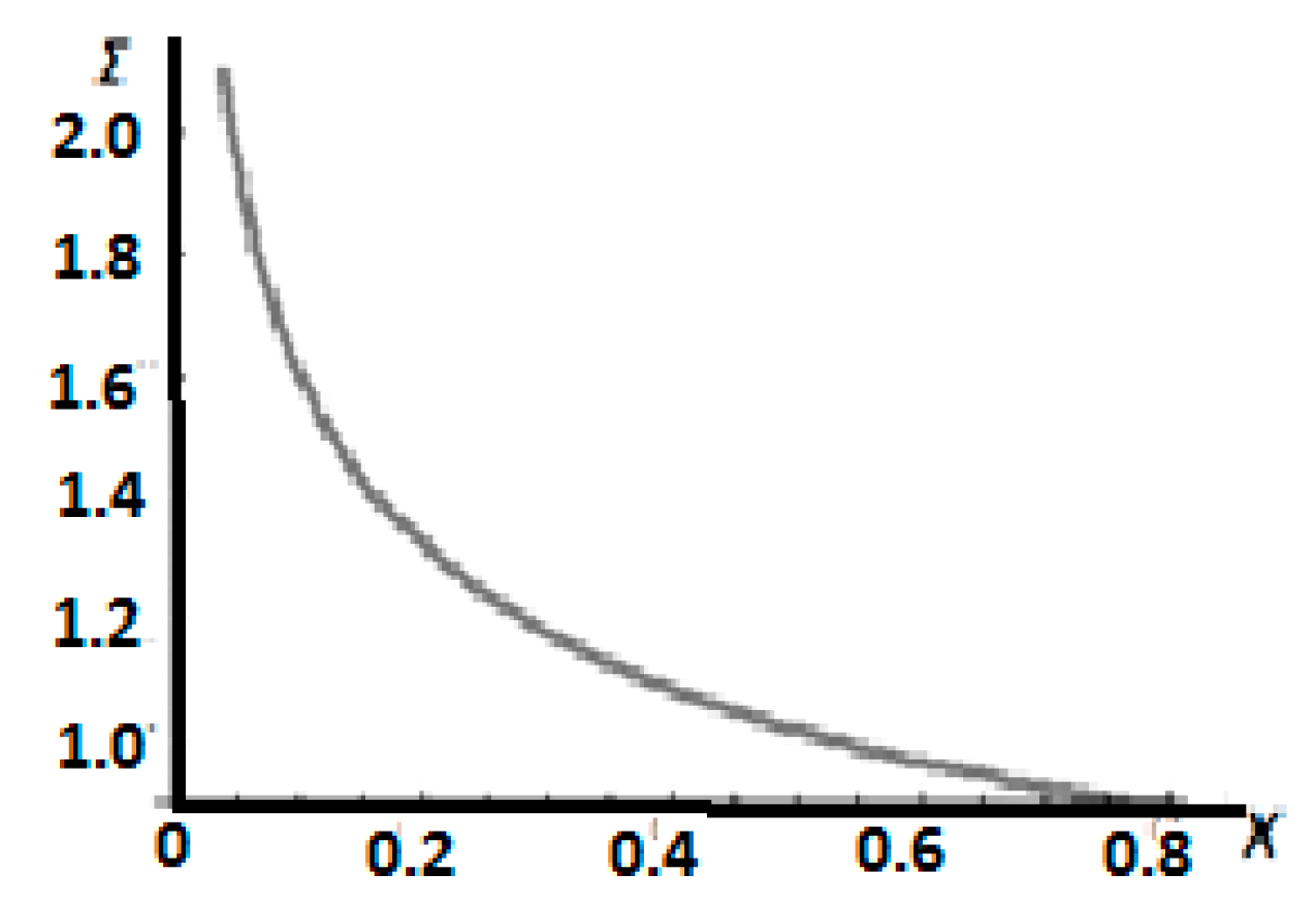
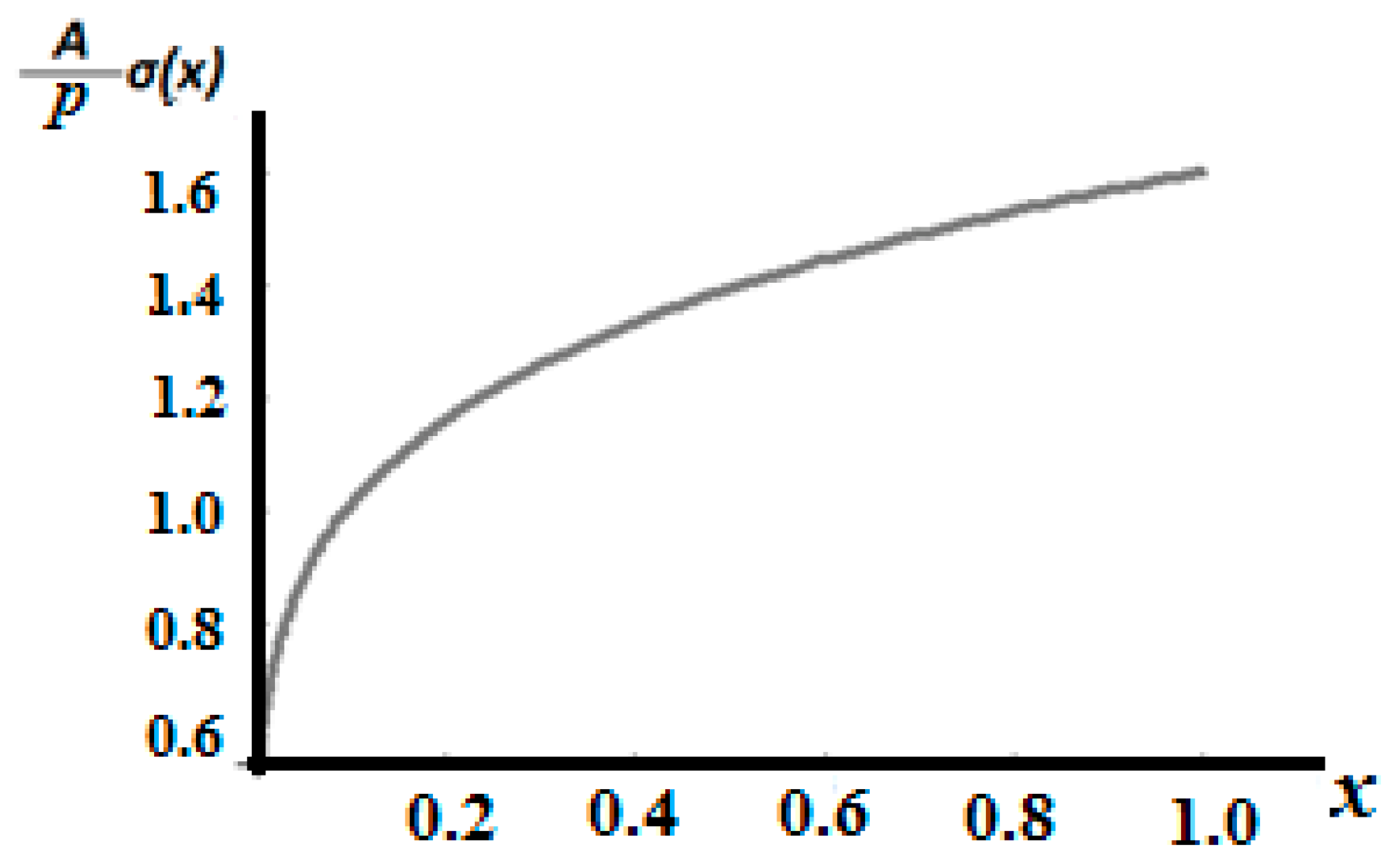
The stress Σ in the dual Λ-fractional space is defined by

$$\Sigma =\frac{P}{A^{\Lambda }}=\frac{1.1270p}{1.199A{X}^{0.2857}}$$

(23)

The non-dimensionalized stress $S=\frac{P}{A^{\Lambda }}\Sigma$ is shown in Figure 4.

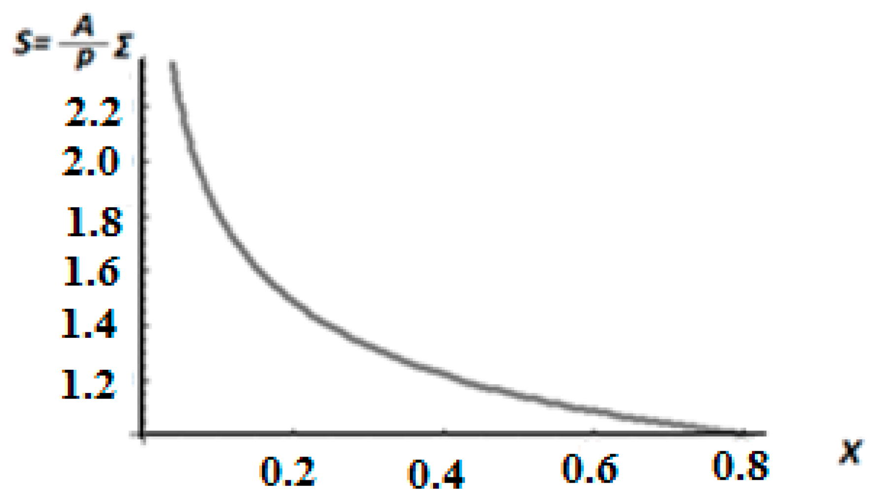
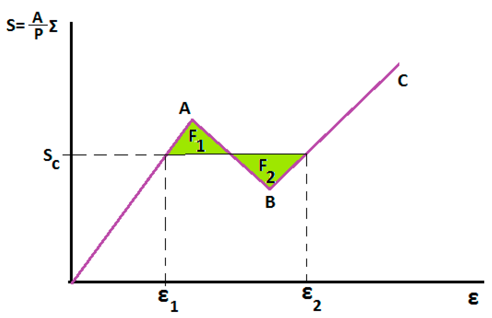
Proceeding to the consideration of the stress S-strain ε diagram in the dual (Λ-space), the critical stress S_c with the corresponding strains ε₁, ε₂, satisfying the Weierstrass–Erdmann jumping conditions in Equations (18) and (19), is shown in Figure 5. Indeed, the areas F₁ and F₂ are equal. That is the geometrical configuration of the Weierstrass–Erdman Equations (18) and (19).

The non-convex stress–strain diagram in the Λ-fractional space is defined with non-dimensional stress,

$$S=\frac{A^{}}{p}\Sigma ,$$

(24)

coexisting stress S_c = 1.5, and the corresponding coexisting strains ε₁ = 0.03 and ε₂ = 0.12. Further, the convex branches of the diagram are parallel. Indeed,

S = E ε for 0 < ε < ε₁

(25)

S = S_c + Ε (ε − ε₂) for ε₂ < ε.

(26)

The fractional stresses are quite high, near the neighborhood of X = 0 since the fractional cross-section area there becomes almost zero. Hence, starting from the point X = 0 with high strains and stresses, the branch BC of Figure 5 is followed. When the stress reaches the coexisting value S_c with strain ε₂, two strains are shown up; the strain ε₁ and the strain ε₂. In that case, the areas F₁ = F₂ in the diagram of Figure 5 are equal. Reducing the stress in the left part of the diagram with the line oA follows.

Therefore, the displacement Y(X) is defined in the branch BC of Figure 5 with the strain ε ≥ ε₂ by the equation

$$\frac{dY\left(X\right)}{dX}=\frac{S}{E}+\left({\epsilon }_2-{\epsilon }_1\right),\hspace{1em}\epsilon \ge {\epsilon }_2$$

(27)

with E denoting Young’s modulus in the dual Λ-space. Then,

$${\rm Y}\left({\rm X}\right)={{\displaystyle \int }}_0^X(\frac{S}{E}+\left({\epsilon }_2-{\epsilon }_1\right))d{\rm X}, 0 < {\rm X}< {{\rm X}}_c.$$

(28)

Further, that distribution of the displacement is valid for the part 0 < X < X_c of the bar, with Χ_c denoting the cross-section of the bar where jumping of the strain takes place and the two stresses ε₁ and ε₂ coexist. Further, Equation (23) yields

$$S=\frac{A}{P}=\frac{1.1270}{1.199X^{0.2857}}.$$

(29)

Then, the point Χ_c, where the coexistence of phases occurs is defined by the equation

$$S_c=\frac{1.1270}{1.199X_c^{0.2857}}.$$

(30)

Consequently, the displacement equation for X_c < X < L is expressed by

$${\rm Y}\left({\rm X}\right)={{\displaystyle \int }}_0^X\frac{S}{E}d{\rm X}+\left(\epsilon 2-\epsilon 1\right)X_c$$

(31)

where (ε₂ − ε₁)Χ is the influence of the coexistence of phases upon displacement. Let us point out that for S_c = 0.15, ε₁ = 0.03 and ε₂ = 0.12 and the non-dimensionalized Young’s modulus E = 50 p/A; then, X_c = 0.195. Considering Equation (29), Equation (28) yields

$$Y\left(X\right)=0.026X^{0.714}+0.09X, 0 < {\rm X}< {{\rm X}}_c.$$

(32)

Further, Equation (31) yields the displacement for 0 < Χ < X_c,

$$Y\left(X\right)=0.026X^{0.714}+0.09X_c.$$

(33)

Yet, the combined displacement field in the Λ-space is shown in Figure 6.

Transferring the functions of the stresses and the displacements in the dual of the dual initial space, that is just the initial space, the variable X should be substituted by

$$X=0.805x^{1.4}$$

(34)

Then, the point of the jumping of the strains at the point X_c = 0.195 is transferred into the initial space with x_c = 0.3632. Further, transferring the stress function Equation (23) from the Λ-space to the initial one,

$$S\left(x\right)=\frac{1.1270p}{1.199A{X}^{0.857}}=\frac{p}{A}{x}^{-0.4}.$$

(35)

Equation (35) yields the stress function S, generated in the Λ-space and expressed in the variable x of the initial space. Then, the stresses in the initial space are expressed as the dual space of S(X) following Equation (9):

$$\sigma \left(x\right)={}_a{}^{RL}D{{}_x^{1-\gamma }}^{}S\left(X\left(x\right)\right)=1.62\frac{p}{A} x^{0.2}.$$

(36)

The distribution of the stresses in the initial space is shown in Figure 7.

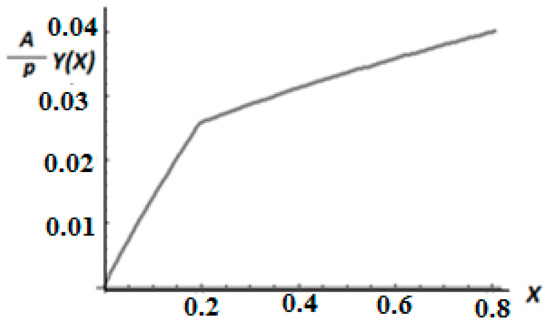
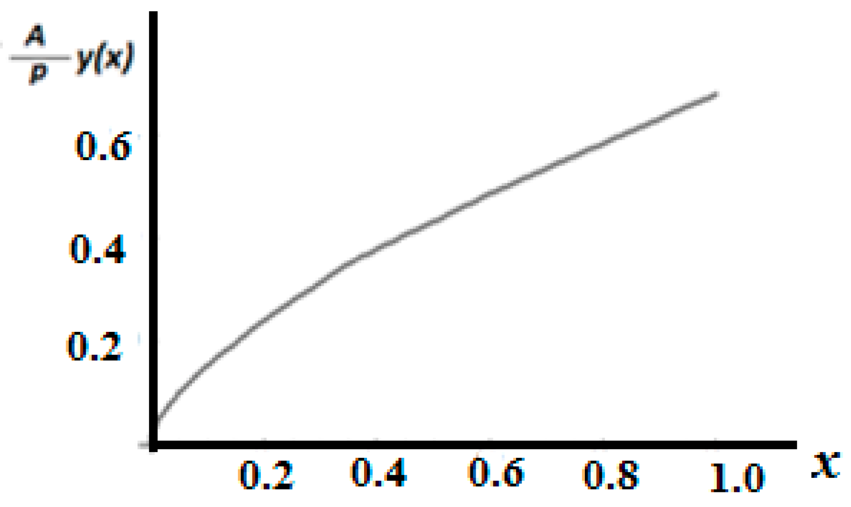
Proceeding to the distribution of the displacements y(x) in the initial space, it is first pointed out that the strains as derivatives of the displacement may not be transferred to the initial space. The displacement function may only be transferred to the initial space as a function of x. Indeed, following the same procedure, the displacement function may be transferred in the dual initial space with

$$y\left(x\right)=0.0263x^{0.714}+0.09x, 0 < x< 0.3632$$

(37)

$$y\left(x\right)=0.0176+0.0263x^{0.714}, 0.3612 < x< 1.$$

(38)

Figure 8 shows the displacement function in the initial space.

The present example may be considered a model for discussing fractional mechanics problems, taking into consideration globally stable equilibrium configurations.

5. Conclusions and Further Research

The stability of Λ-fractional bars is discussed. It is suggested that the stability criterion should not be local in the context of Λ-fractional analysis, which is inherently global. Hence, variational approaches, with corner Weierstrass-Erdman conditions, may be recalled and applied. Those conditions yield deformations, with non-smooth strains exhibiting the co-existence of phases phenomenon. The present work should be considered as a model for discussing stability and equilibrium in the context of Λ-fractional analysis. The dynamic response of the bars, exhibiting the co-existence of phases phenomenon, is considered as an extension of the proposed globally stable configurations of the equilibrium problem. The impact problem will also be considered as an extension of the present theory. The proposed theory may be applied to any problem demanding fractional analysis, for example problems in micro- and nano- mechanics and physics, bioengineering, medical engineering, signal processing, liquid crystals, etc. Further, fractional variational procedures are acceptable only when they are searching for global extremals, with the consideration of the corner conditions.