Using Laplace Residual Power Series Method in Solving Coupled Fractional Neutron Diffusion Equations with Delayed Neutrons System

Abstract

In this paper, a system of coupled fractional neutron diffusion equations with delayed neutrons was solved efficiently by using a combination of residual power series and Laplace transform techniques, and the anomalous diffusion was considered by taking the non-Gaussian case with different values of fractional parameter α. The Laplace residual power series method (LRPSM) does not require differentiation, conversion, or discretization for the assumed conditions, so the approach is simple and suitable for solving higher-order fractional differential equations. To assure the theoretical results, two different neutron flux initial conditions were presented numerically, where the needed Mathematica codes were performed using essential nuclear reactor cross-section data, and the results for different values of times were tabulated and graphically figured out. Finally, it must be noted that the results align with the Adomian decomposition method.

1. Introduction

The revolution of using energy generated from nuclear reactors can be considered as an essential part of a clean renewable source of energy; today, nuclear reactors cover 10% of the use of the global needed energy.

The inspiring idea is that the creation of nuclear energy is released when heavy nuclei undergo fission while they are bombarded by (thermal) slow neutrons. The neutron diffusion equation, which is simplified from the neutron transport equation when using Fick’s law, describes the behavior of neutrons in the nuclear fission reactor [1,2,3]. Researchers have investigated their scientific ambitions by studying different issues in this field, where different cases of neutron diffusion equations have been solved by various techniques. The homotopy perturbation method (HPM) has been used in solving bare hemispherical symmetry and cylindrical symmetry one group neutron diffusion equation reactors [4,5]; the residual power series method was used to solve multi-energy groups of neutron diffusion equations [6,7]; then the HPM is used to solve reflected reactor one group different geometries neutron diffusion equations; finally, solving a multi-group reflected spherical reactor system of equations using the HPM is performed [8].

The distribution of neutrons in nuclear reactors is constructed in the same way as dissolving the solute in the chemical solutions, which can be represented mathematically by the continuity equation:

$$\frac{1}{v_c}\frac{\partial \psi \left(\mathit{r},t\right)}{\partial t}=s\left(\mathit{r},t\right)-{\Sigma }_a\psi \left(\mathit{r},t\right)-\mathsf{\nabla }·\mathit{J}\left(\mathit{r},t\right),$$

(1)

where $\psi \left(\mathit{r},t\right)$ is the neutron flux; $\mathit{J}\left(\mathit{r},t\right)$ is neutron current density; ${\sum }_a$ is the macroscopic absorption cross-section; $v_c$ is neutron velocity; and $s\left(\mathit{r},t\right)$ is a source of neutrons term. Using Fick’s law, which gives the relation between neutron flux $\psi \left(\mathit{r}, t\right)$ and the current density $\mathit{J}\left(\mathit{r},t\right):$

$$\mathit{J}\left(\mathit{r}, t\right)=-D\mathsf{\nabla }\psi \left(\mathit{r}, t\right)$$

(2)

where D is the neutron diffusion coefficient, then the neutron diffusion equation can be expressed as

$$\frac{1}{v_c}\frac{\partial \psi \left(\mathit{r},t\right)}{\partial t}=s\left(\mathit{r}, t\right)-{\Sigma }_a \psi \left(\mathit{r},t\right)+D{\mathsf{\nabla }}^2\psi \left(\mathit{r}, t\right).$$

(3)

This is the well-known nuclear reactor time-dependent neutron diffusion equation.

One step forward, the fractional study of the time-dependent neutron diffusion equation is to make the situation more detailed by studying the physical effect of delayed neutrons. These delayed neutrons have an essential role in the reactor. Investigating a system of coupled fractional neutron diffusion equations with delayed neutrons was the target of this work.

The importance of delayed neutrons in reactors is the effective lifetime of such neutrons (which are given by their prompt lifetime, and additional delayed time), which is characterized by the β-decay of their precursor, which is considerably longer than the prompt neutron lifetime. Hence, delayed neutrons substantially increase the time constant of a reactor so that effective control is possible.

The contribution of the effect of the delayed neutron is included in Equation (3) in the source term $s\left(\mathit{r},t\right)$, which can be written as

$$s\left(\mathit{r},t\right)=\mathsf{\gamma }{\sum }_f \psi \left(\mathit{r},t\right)+\lambda c\left(\mathit{r},t\right)$$

(4)

In this study, the general three-dimension vector $\mathit{r}$ will be simplified to the one-dimension vector $x$ to be more suitable.

The system of time-dependent neutron diffusion equations is known as the neutron point kinetic model; this is in one dimension:

$$\frac{1}{v_c}\frac{\partial }{\partial t}\psi \left(x,t\right)=D\frac{{\partial }^2}{\partial x^2}\psi \left(x,t\right)+\left(-{\sum }_a+\gamma {\sum }_f\right)\psi \left(x,t\right)+\lambda c\left(x,t\right),$$

(5)

$$\frac{\partial }{\partial t}c\left(x,t\right)=\beta \nu {\sum }_f \psi \left(x,t\right)-\lambda c\left(x,t\right),$$

(6)

with initial conditions:

$$\psi \left(x,0\right)={\psi }_0\left(x\right), c\left(x,0\right)=\frac{\beta \mathsf{\gamma }{\sum }_f}{\lambda }{\psi }_0\left(x\right).$$

(7)

where the delayed neutron density is $c\left(x,t\right)$, and the constants γ, λ, and β are the average number of neutrons produced per fission, the radioactive decay constant, and the fraction of the delayed fission neutrons, respectively, where $\left(-{\sum }_a+\mathsf{\gamma }{\sum }_f\right)$ can be considered as the total macroscopic cross-section $\sum$.

The kinetic equation describes the dynamics of space-time neutron distribution in the reactors. These equations are divided into point kinetic equations and space kinetic equations; the time change in neutron density is described by the kinetic point equations, which estimate the reactor power response; the fractional calculus governs an important part of the time-dependent diffusion equation in the presence of delayed neutrons, which is known as anomalous diffusion; the anomalous diffusion is called by the variation from the Gaussian distribution of the diffusion.

Anomalous diffusion is characterized by the asymptotical nonlinear (especially power-law type) dependence of the mean-squared displacement on the time, which is $⟨x^2\left(t\right)⟩~t^{\alpha }$.

The parameter α feeds back in the determination of the type of fractional neutron diffusion equation, where the anomalous diffusion ($\alpha \ne 1)$ is classified into sub diffusion ($\alpha <1$) and super diffusion ($\alpha >1$).

In the case of α = 1: the diffusion is Gaussian, mathematically representing the non-fractional neutron diffusion equation.

The trapping of neutrons in the medium causes slower neutron movement considered as sub diffusion, while the fast movement of neutrons when they move in one direction for a very long time without any collision is characterized by super diffusion [9,10].

The fractional neutron diffusion equation with a delayed neutron system has been studied in many works where the fractional two energy group matrix representation for nuclear reactor dynamics with an external source is considered [11], while the coupled fractional neutron diffusion equations with delayed neutrons have been solved [12], and an exact solution in the case of the one-dimensional neutron diffusion kinetic equation with one delayed precursor concentration in Cartesian geometry was studied [13].

Here, the fractional neutron diffusion equations with one delayed neutron group can be written as follows:

$$\frac{1}{v_c}{\mathfrak{D}}_t^{\alpha }\psi \left(x,t\right)=D{\mathsf{\nabla }}^2\psi \left(x,t\right)+\left(\gamma {\sum }_f-{\sum }_a\right) \psi \left(x,t\right)+\lambda c\left(x,t\right),$$

(8)

$${\mathfrak{D}}_t^{\alpha }c\left(x,t\right)=\beta \gamma {\sum }_f \psi \left(x,t\right)-\lambda c\left(x,t\right),$$

(9)

$$\psi \left(x,0\right)={\psi }_0\left(x\right),c\left(x,0\right)=\frac{\beta \gamma {\sum }_f}{\lambda }{\psi }_0\left(x\right).$$

(10)

Numerous numerical and analytical techniques including Laplace transforms, the homotopy method, the Pade-variational iteration method, the finite difference method, the Adomian decomposition method, and others [14,15,16,17,18,19,20,21,22,23,24] have been developed to solve fractional differential equations. However, these methods have limitations such as the need for long and complex computations. Therefore, they need to be connected to a transform operator. The authors of [25] combined the residual power series method (RPSM) with the Laplace transform to introduce actual and series solutions of the linear and nonlinear FDEs. The new method, known as the Laplace-residual power series method (LRPSM), was adopted to construct series solutions of a variety of fractional deferential equations (FDEs). LRPSM does not rely on fractional derivation to determine the coefficients of the series as in RPSM, but depends on the concept of the limit, so few calculations generate the coefficients compared to the residual power series method. The current technique is quick, requires little computer memory, and is not influenced by computational round-off errors. Furthermore, this technique computes the coefficients of the power series using a chain of equations with more than one variable, indicating that the present method has a rapid convergence.

This paper solved a system of coupled fractional neutron diffusion equations with delayed neutrons efficiently by applying LRPSM. The accuracy and effectiveness of the method were clarified by displaying numerical examples and comparing the solutions with the results of some approved approaches.

The rest of paper is structured as follows. The concepts and theorems in fractional calculus and Laplace transforms that are required to reach our results are introduced in Section 2. The LRPSM algorithm is described in Section 3. Section 4 introduces the numerical examples and compares the solutions with the results of some approved approaches. In Section 5, we finally present our conclusions.

2. Fractional Expansion in Laplace Space

The fractional derivatives are non-local operators because they are defined using integrals. Therefore, the time-fractional derivative contains information about the function at earlier points, thus it possesses a memory effect. Such derivatives consider the history and non-local distributed effects, which are essential for better and more accurate descriptions and an understanding of complex and dynamic system behavior.

The fractional calculus in Caputo’s sense and the Laplace transform, which are necessary to create the LRPS solution for the fractional neutron diffusion equations with one delayed neutron group, are introduced in this part with some basic concepts and ideas.

Definition 1.

The time-fractional Caputo derivative of order $\alpha$ of $\psi \left(x,t\right)$ sense is defined as

$${\mathfrak{D}}_t^{\alpha }\psi \left(x,t\right)=J_t^{n-\alpha }{\partial }_t^n\psi \left(x,t\right), n-1<\alpha \le n, x\in I. t>0,$$

(11)

where ${\mathfrak{D}}_t^{\alpha }$ denotes the time-fractional Caputo derivative operator of order $\alpha$; $n\in \mathbb{N}$;$I$ is an interval; and$J_t^{\beta }$ is the time-fractional Riemann–Liouville integral operator of order $\beta$ that is defined as:

$$J_t^{\beta }\psi \left(x,t\right)=\left\{\begin{array}{c}\frac{1}{\Gamma \left(\beta \right)}\underset{0}{\overset{t}{{\displaystyle \int }}}{\left(t-\tau \right)}^{\beta -1}\psi \left(x,\tau \right)d\tau , \beta >0 , t>\tau \ge 0\\ \psi \left(x,t\right), \beta =0\end{array}\right.,$$

(12)

In the following lemma, we introduce certain properties of the operator ${\mathfrak{D}}_t^{\alpha }$ that we will require for the rest of the work in this paper. The reader should see [26] for more features.

Lemma 1.

For$n-1<\alpha \le n$,$\epsilon >-1, t\ge 0$, and$\mu \in ℝ$, we have:

$$\begin{array}{l}(i) {\mathfrak{D}}_t^{\alpha }{t}^{\epsilon }=\frac{\Gamma \left(\epsilon +1\right)}{\Gamma \left(\epsilon +1-\alpha \right)}{t}^{\epsilon -\alpha },\\ \left(\mathrm{ii}\right) \begin{array}{c}{\mathfrak{D}}_t^{\alpha }\mu =0\end{array},\\ \left(\mathrm{iii}\right) {\mathfrak{D}}_t^{\alpha }{J}_t^{\alpha }\psi \left(x,t\right)=\psi \left(x,t\right),\\ (\mathrm{iv}) J_t^{\alpha }{\mathfrak{D}}_t^{\alpha }\psi \left(x,t\right)=\psi \left(x,t\right)-{{\displaystyle \sum }}_{j=0}^{n-1}{\partial }_t^j\psi \left(x,0^{+}\right)\frac{t^j}{j!}.\end{array}$$

(13)

Definition 2.

Let$\psi \left(x,t\right)$be a continuous function on$I\times \left[0,\infty \right)$and of exponential order$\delta$. Then, the Laplace transform of the function$\psi \left(x,t\right)$is denoted and defined as follows:

$$\mathsf{\Psi }\left(x,s\right)=\mathcal{L}\left[\psi \left(x,t\right)\right]≔\underset{0}{\overset{\infty }{{\displaystyle \int }}}{e}^{-st}\psi \left(x,t\right)dt, s>\delta ,$$

(14)

whereas the inverse Laplace transform of the function$\mathsf{\Psi }\left(x,s\right)$is defined as follows:

$$\psi \left(x,t\right)={\mathcal{L}}^{-1}\left[\mathsf{\Psi }\left(x,s\right)\right]≔\underset{c-i\infty }{\overset{c+i\infty }{{\displaystyle \int }}}{e}^{st}\mathsf{\Psi }\left(x,s\right)ds,c=Re\left(s\right)>c_0,$$

(15)

where$c_0$lies in the right half plane of the absolute convergence of the Laplace integral.

In the next lemma, we introduce several crucial characteristics related to the Laplace transform and the fractional derivative in the Caputo sense.

Lemma 2.

Let $\psi \left(x,t\right)$ be a continuous function on$I\times \left[0,\infty \right)$and of exponential orders$\delta$, and $\mathsf{\Psi }\left(x,s\right)=\mathcal{L}\left[\psi \left(x,t\right)\right]$. Then,

$$\begin{array}{l}(\mathrm{i}) \underset{s\to \infty }{\lim }s\mathsf{\Psi }\left(x,s\right)=\psi \left(x,0\right), x\in I;\\ \left(\mathrm{ii}\right) \mathcal{L}\left[ J_t^{\alpha }\psi \left(x,t\right)\right]=s^{\alpha -1}\mathsf{\Psi }\left(x,s\right), \alpha >0;\\ \left(\mathrm{iii}\right) \mathcal{L}\left[{\mathfrak{D}}_t^{\alpha }\psi \left(x,t\right)\right]=s^{\alpha }\mathsf{\Psi }\left(x,s\right)-{{\displaystyle \sum }}_{k=0}^{n-1}{s}^{\alpha -k-1}{\partial }_t^k\psi \left(x,0\right), n-1<\alpha <n;,\\ (\mathrm{iv}) \mathcal{L}\left[{\mathfrak{D}}_t^{m\alpha }\psi \left(x,t\right)\right]=s^{m\alpha }\mathsf{\Psi }\left(x,s\right)-{{\displaystyle \sum }}_{k=0}^{m-1}{s}^{\left(m-k\right)\alpha -1}{\mathfrak{D}}_t^{k\alpha }\psi \left(x,0\right),0<\alpha <1.\end{array}$$

(16)

where ${\mathfrak{D}}_t^{m\alpha }={\mathfrak{D}}_t^{\alpha }·{\mathfrak{D}}_t^{\alpha }\dots {\mathfrak{D}}_t^{\alpha }$($m$-times)$.$

Now, as shown in the following result, we add a new fractional expansion that serves as the foundation for creating a LRPS solution for the partial differential equations (PDEs).

Theorem 1.

Let $\psi \left(x,t\right)$ be continuous on $I\times \left[0,\infty \right)$ and of exponential order $\delta$. Suppose that the function$\mathsf{\Psi }\left(x,s\right)=\mathcal{L}\left[\psi \left(x,t\right)\right]$has the following fractional expansion:

$$\mathsf{\Psi }\left(x,s\right)={\displaystyle \sum }_{n=0}^{\infty }\frac{f_n\left(x\right)}{s^{n\alpha +1}}, 0<\alpha \le 1, x\in I, s>\delta ,$$

(17)

then $f_n\left(x\right)={\mathfrak{D}}_t^{n\alpha }\psi \left(x,0\right)$.

The following theorem shows the conditions that guarantee the convergence of the series in the expansion (17).

Theorem 2.

Let $\psi \left(x,t\right)$ be a continuous function on $\mathrm{I}\times \left[0,\infty \right)$ and of exponential order $\delta$ and $\mathsf{\Psi }\left(x,s\right)=\mathcal{L}\left[\psi \left(x,t\right)\right]$ can be represented as the fractional expansion in Theorem 1. If $\left|\mathrm{s} \mathcal{L}\left[{\mathfrak{D}}_{\mathrm{t}}^{\left(n+1\right)\mathsf{\alpha }}\psi \left(x,t\right)\right]\right|\le \mathrm{M}\left(x\right),$on $I\times \left(\delta ,\right.\left.\gamma \right]$ where $0<\mathsf{\alpha }\le 1$, then the remainder ${\mathrm{R}}_{\mathrm{n}}\left(\mathrm{x},\mathrm{s}\right)$ of the fractional expansion as in Equation (17) satisfies the following inequality:

$$\left|R_n\left(x,s\right)\right|\le \frac{M\left(x\right), }{s^{\left(n+1\right)\alpha +1}} , x\in I, \delta <s\le \gamma$$

.

3. Exact Solution of the Fractional Neutron Diffusion Equations with One Delayed Neutron Group

The main objective of this section is to implement the LRPSM to construct a series solution to the fractional neutron diffusion equations with one delayed neutron group

$$\begin{gathered} \frac{1}{v_c}{\mathfrak{D}}_t^{\alpha }\psi \left(x,t\right)=D{\mathsf{\nabla }}^2\psi \left(x,t\right)+\left(\gamma {\sum }_f-{\sum }_a\right) \psi \left(x,t\right)+\lambda c\left(x,t\right), \\ {\mathfrak{D}}_t^{\alpha }c\left(x,t\right)=\beta \gamma {\sum }_f \psi \left(x,t\right)-\lambda c\left(x,t\right), \end{gathered}$$

(18)

with the initial conditions

$$\psi \left(x,0\right)={\psi }_0\left(x\right), c\left(x,0\right)=\frac{\beta \nu {\sum }_f}{\lambda }{\psi }_0\left(x\right),$$

(19)

Rewriting the coupled equations in (18) by replacing $B=\beta \gamma {\sum }_f$ and $\sum =\gamma {\sum }_f-{\sum }_a,$ we obtain

$$\begin{gathered} {\mathfrak{D}}_t^{\alpha }\psi \left(x,t\right)=v_c D {\psi }_{xx}\left(x,t\right)+v_c \sum \psi \left(x,t\right)+v_c\lambda c\left(x,t\right), \\ {\mathfrak{D}}_t^{\alpha }c\left(x,t\right)=B\psi \left(x,t\right)-\lambda c\left(x,t\right), \end{gathered}$$

(20)

with the initial conditions

$$\psi \left(x,0\right)={\psi }_0\left(x\right), c\left(x,0\right)=\frac{B}{\lambda }{\psi }_0\left(x\right),$$

(21)

Operating the Laplace transform on the coupled equations in (20), we obtain

$$\begin{gathered} \mathcal{L}\left[{\mathfrak{D}}_t^{\alpha }\psi \left(x,t\right)\right]=v_c D \mathcal{L} \left[{\psi }_{xx}\left(x,t\right)\right]+v_c \sum \mathcal{L}\left[\psi \left(x,t\right)\right]+v_c\lambda \mathcal{L}\left[c\left(x,t\right)\right], \\ \mathcal{L}\left[{\mathfrak{D}}_t^{\alpha }c\left(x,t\right)\right]=B\left[\psi \left(x,t\right)\right]-\lambda \mathcal{L}\left[c\left(x,t\right)\right]. \end{gathered}$$

(22)

According to Lemma 2 part (iii) and using the initial conditions in Equation (21), we can write equations in (22) in the following form:

$$\begin{gathered} s^{\alpha }\Psi \left(x,s\right)-s^{\alpha -1}{\psi }_0\left(x\right)=v_c D {\Psi }_{xx}\left(x,s\right)+v_c \sum \Psi \left(x,s\right)+v_c\lambda C\left(x,s\right), \\ {s}^{\alpha }C\left(x,s\right)-s^{\alpha -1}\frac{B}{\lambda }{\psi }_0\left(x\right)=B\Psi \left(x,s\right)-\lambda C\left(x,s\right), \end{gathered}$$

(23)

where $\Psi \left(x,s\right)=\mathcal{L}\left[\psi \left(x,t\right)\right],$ $C\left(x,s\right)=\mathcal{L}\left[c\left(x,t\right)\right].$

Equation (23) can be written as

$$\begin{gathered} \Psi \left(x,s\right)-\frac{1}{s}{\psi }_0\left(x\right)-\frac{v_c D}{s^{\alpha }} {\Psi }_{xx}\left(x,s\right)-\frac{v_c \sum }{s^{\alpha }} \Psi \left(x,s\right)-\frac{v_c\lambda }{s^{\alpha }} C\left(x,s\right)=0, \\ C\left(x,s\right)-\frac{B}{\lambda s}{\psi }_0\left(x\right)-\frac{B}{s^{\alpha }} \Psi \left(x,s\right)+\frac{\lambda }{s^{\alpha }} C\left(x,s\right)=0. \end{gathered}$$

(24)

The coupled equations in Equation (24) represent a linear system of partial differential equations that contain derivatives relative to the independent variable $x$. According to the Laplace residual power series method, we assume that the series solution of the system in Equation (24) has the form

$$\begin{gathered} \Psi \left(x,s\right)={\displaystyle \sum }_{n=0}^{\infty }\frac{f_n\left(x\right)}{s^{n\alpha +1}},x\in I, s>\delta \ge 0, \\ C\left(x,s\right)={\displaystyle \sum }_{n=0}^{\infty }\frac{g_n\left(x\right)}{s^{n\alpha +1}},x\in I, s>\delta \ge 0. \end{gathered}$$

(25)

Using the fact in Lemma 2 part (i), of the kth truncated series of $\mathsf{\Psi }\left(x,s\right),C\left(x,s\right)$ can be expressed as

$$\begin{gathered} {\Psi }_k\left(x,s\right)=\frac{{\psi }_0\left(x\right)}{s}+{\displaystyle \sum }_{n=1}^k\frac{f_n\left(x\right)}{s^{n\alpha +1}},x\in I, s>\delta \ge 0, \\ {C}_k\left(x,s\right)=\frac{B}{\lambda s}{\psi }_0\left(x\right)+{\displaystyle \sum }_{n=1}^k\frac{g_n\left(x\right)}{s^{n\alpha +1}},x\in I, s>\delta \ge 0. \end{gathered}$$

(26)

In the next step, we define the Laplace residual functions of the coupled equations in (24) in order to find the unknown coefficients of the series in Equation (26):

$$\begin{gathered} LRes\left(\Psi \left(x,s\right)\right)=\Psi \left(x,s\right)-\frac{1}{s}{\psi }_0\left(x\right)-\frac{v_c D}{s^{\alpha }} {\Psi }_{xx}\left(x,s\right)-\frac{v_c \sum }{s^{\alpha }} \Psi \left(x,s\right)-\frac{v_c\lambda }{s^{\alpha }} C\left(x,s\right), \\ LRes\left(C\left(x,s\right)\right)=C\left(x,s\right)-\frac{B}{\lambda s}{\psi }_0\left(x\right)-\frac{B}{s^{\alpha }} \Psi \left(x,s\right)+\frac{\lambda }{s^{\alpha }} C\left(x,s\right). \end{gathered}$$

(27)

and the kth Laplace-residual functions as

$$\begin{gathered} LRe{s}_k\left(\Psi \left(x,s\right)\right)={\Psi }_k\left(x,s\right)-\frac{1}{s}{\psi }_0\left(x\right)-\frac{v_c D}{s^{\alpha }} {\Psi }_k{}_{xx}\left(x,s\right)-\frac{v_c \sum }{s^{\alpha }} {\Psi }_k\left(x,s\right)-\frac{v_c\lambda }{s^{\alpha }} C_k\left(x,s\right), \\ LRe{s}_k\left(C\left(x,s\right)\right)=C_k\left(x,s\right)-\frac{B}{\lambda s}{\psi }_0\left(x\right)-\frac{B}{s^{\alpha }} {\Psi }_k\left(x,s\right)+\frac{\lambda }{s^{\alpha }} C_k\left(x,s\right). \end{gathered}$$

(28)

Since $LRes\left(\mathsf{\Psi }\left(x,s\right)\right)=0$ and $LRes\left(C\left(x,s\right)\right)=0$, we have $s^{k\alpha +1}LRes\left(\mathsf{\Psi }\left(x,s\right)\right)=0, s^{k\alpha +1}LRes\left(C\left(x,s\right)\right)=0$. Therefore,

$$\underset{s\to \infty }{\lim }\left(s^{k\alpha +1}LRe{s}_k\left(\Psi \left(x,s\right)\right)\right)=0, \underset{s\to \infty }{\lim }\left(s^{k\alpha +1}LRe{s}_k\left(C\left(x,s\right)\right)\right)=0 \mathit{for} k=0,1,2,\dots .$$

(29)

To find $f_1\left(x\right)$ and $g_1\left(x\right)$ in Equation (26), we substituted ${\mathsf{\Psi }}_1\left(x,s\right)=\frac{{\psi }_0\left(x\right)}{s}+\frac{f_1\left(x\right)}{s^{\alpha +1}}$ and $C_1\left(x,s\right)=\frac{B}{\lambda s}{\psi }_0\left(x\right)+\frac{g_1\left(x\right)}{s^{\alpha +1}}$ in the first Laplace-residual functions to obtain

$$\begin{gathered} LRe{s}_1\left(\Psi \left(x,s\right)\right)=\frac{f_1\left(x\right)}{s^{\alpha +1}}-\frac{v_c D}{s^{\alpha }} \left[\frac{{\psi }_0^{″}\left(x\right)}{s}+\frac{f_1^{″}\left(x\right)}{s^{\alpha +1}}\right]-\frac{v_c \sum }{s^{\alpha }} \left[\frac{{\psi }_0\left(x\right)}{s}+\frac{f_1\left(x\right)}{s^{\alpha +1}}\right]-\frac{v_c\lambda }{s^{\alpha }} \left[\frac{B}{\lambda s}{\psi }_0\left(x\right)+\frac{g_1\left(x\right)}{s^{\alpha +1}}\right], \\ LRe{s}_1\left(C\left(x,s\right)\right)=\frac{g_1\left(x\right)}{s^{\alpha +1}}-\frac{B}{s^{\alpha }} \left[\frac{{\psi }_0\left(x\right)}{s}+\frac{f_1\left(x\right)}{s^{\alpha +1}}\right]+\frac{\lambda }{s^{\alpha }} \left[\frac{B}{\lambda s}{\psi }_0\left(x\right)+\frac{g_1\left(x\right)}{s^{\alpha +1}}\right]. \end{gathered}$$

(30)

Next, by solving $\underset{s\to \infty }{lim}{s}^{\alpha +1}LRe{s}_1\left(\mathsf{\Psi }\left(x,s\right)\right)=0$,$\underset{s\to \infty }{ lim}{s}^{\alpha +1}LRe{s}_1\left(C\left(x,s\right)\right)=0,$ one can obtain

$$f_1\left(x\right)=v_c D {\psi }_0^{″}\left(x\right)+v_c \sum {\psi }_0\left(x\right)+v_{c}B{\psi }_0\left(x\right),$$

(31)

$$g_1\left(x\right)=0.$$

(32)

To find $f_2\left(x\right)$ and $g_2\left(x\right)$ in Equation (26), we substituted ${\mathsf{\Psi }}_2\left(x,s\right)=\frac{{\psi }_0\left(x\right)}{s}+\frac{f_1\left(x\right)}{s^{\alpha +1}}+\frac{f_2\left(x\right)}{s^{2\alpha +1}}$ and $C_2\left(x,s\right)=\frac{B}{\lambda s}{\psi }_0\left(x\right)+\frac{g_2\left(x\right)}{s^{2\alpha +1}}$ in the second Laplace-residual functions to obtain

$$\begin{gathered} LRe{s}_2\left(\Psi \left(x,s\right)\right)=\frac{f_1\left(x\right)}{s^{\alpha +1}}+\frac{f_2\left(x\right)}{s^{2\alpha +1}}-\frac{v_c D}{s^{\alpha }} \left[\frac{{\psi }_0^{″}\left(x\right)}{s}+\frac{f_1^{″}\left(x\right)}{s^{\alpha +1}}+\frac{f_2^{″}\left(x\right)}{s^{2\alpha +1}}\right]-\frac{v_c \sum }{s^{\alpha }} \left[\frac{{\psi }_0\left(x\right)}{s}+\frac{f_1\left(x\right)}{s^{\alpha +1}}+\frac{f_2\left(x\right)}{s^{2\alpha +1}}\right]-\frac{v_c\lambda }{s^{\alpha }} \left[\frac{B}{\lambda s}{\psi }_0\left(x\right)+\frac{g_2\left(x\right)}{s^{2\alpha +1}}\right], \\ LRe{s}_2\left(C\left(x,s\right)\right)=\frac{g_2\left(x\right)}{s^{2\alpha +1}}-\frac{B}{s^{\alpha }} \left[\frac{{\psi }_0\left(x\right)}{s}+\frac{f_1\left(x\right)}{s^{\alpha +1}}+\frac{f_2\left(x\right)}{s^{2\alpha +1}}\right]+\frac{\lambda }{s^{\alpha }} \left[\frac{B}{\lambda s}{\psi }_0\left(x\right)+\frac{g_2\left(x\right)}{s^{2\alpha +1}}\right]. \end{gathered}$$

(33)

Next, by solving $\underset{s\to \infty }{lim}{s}^{2\alpha +1}LRe{s}_2\left(\mathsf{\Psi }\left(x,s\right)\right)=0$,$\underset{s\to \infty }{ lim}{s}^{2\alpha +1}LRe{s}_2\left(C\left(x,s\right)\right)=0,$ one can obtain

$$f_2\left(x\right)=v_c D f_1^{″}\left(x\right)+v_c \sum f_1\left(x\right),$$

(34)

$$g_2\left(x\right)=B{f}_1\left(x\right).$$

(35)

In the third Laplace, the residual functions to obtain

$$\begin{gathered} LRe{s}_3\left(\Psi \left(x,s\right)\right)=\frac{f_1\left(x\right)}{s^{\alpha +1}}+\frac{f_2\left(x\right)}{s^{2\alpha +1}}+\frac{f_3\left(x\right)}{s^{3\alpha +1}}-\frac{v_c D}{s^{\alpha }} \left[\frac{{\psi }_0^{″}\left(x\right)}{s}+\frac{f_1^{″}\left(x\right)}{s^{\alpha +1}}+\frac{f_2^{″}\left(x\right)}{s^{2\alpha +1}}+\frac{f_3^{″}\left(x\right)}{s^{3\alpha +1}}\right]-\frac{v_c \sum }{s^{\alpha }} \left[\frac{{\psi }_0\left(x\right)}{s}+\frac{f_1\left(x\right)}{s^{\alpha +1}}+\frac{f_2\left(x\right)}{s^{2\alpha +1}}+\frac{f_3\left(x\right)}{s^{3\alpha +1}}\right]-\frac{v_c\lambda }{s^{\alpha }} \left[\frac{B}{\lambda s}{\psi }_0\left(x\right)+\frac{g_2\left(x\right)}{s^{2\alpha +1}}+\frac{g_3\left(x\right)}{s^{3\alpha +1}}\right], \\ LRe{s}_3\left(C\left(x,s\right)\right)=\frac{g_2\left(x\right)}{s^{2\alpha +1}}+\frac{g_3\left(x\right)}{s^{3\alpha +1}}-\frac{B}{s^{\alpha }} \left[\frac{{\psi }_0\left(x\right)}{s}+\frac{f_1\left(x\right)}{s^{\alpha +1}}+\frac{f_2\left(x\right)}{s^{2\alpha +1}}+\frac{f_3\left(x\right)}{s^{3\alpha +1}}\right]+\frac{\lambda }{s^{\alpha }} \left[\frac{B}{\lambda s}{\psi }_0\left(x\right)+\frac{g_2\left(x\right)}{s^{2\alpha +1}}+\frac{g_3\left(x\right)}{s^{3\alpha +1}}\right]. \end{gathered}$$

(36)

By solving $\underset{s\to \infty }{lim}{s}^{3\alpha +1}LRe{s}_3\left(\mathsf{\Psi }\left(x,s\right)\right)=0$,$\underset{s\to \infty }{ lim}{s}^{3\alpha +1}LRe{s}_3\left(C\left(x,s\right)\right)=0,$ one obtains

$$f_3\left(x\right)=v_c D f_2^{″}\left(x\right)+v_c \sum f_2\left(x\right)+v_c\lambda g_2\left(x\right),$$

(37)

$$g_3\left(x\right)=B{f}_2\left(x\right)-\lambda g_2\left(x\right).$$

(38)

If we continue in the same manner, we can substitute the k^th truncated series ${\mathsf{\Psi }}_k\left(x,s\right)$,$C_k\left(x,s\right)$ into the k^th Laplace-residual function $LRe{s}_k\left(\mathsf{\Psi }\left(x,s\right)\right), LRe{s}_k\left(C\left(x,s\right)\right)$. Then, we can multiply the resulting equations by $s^{k\alpha +1}$ and taking the limit as $s\to \infty$, $f_{k+1}\left(x\right)$, $g_{k+1}\left(x\right)$ for $k\ge 2$ can be obtained by the following recurrence relation:

$$f_n\left(x\right)=v_c D f_{n-1}^{″}\left(x\right)+v_c \sum f_{n-1}\left(x\right)+v_c\lambda g_{n-1}\left(x\right),$$

(39)

$$g_n\left(x\right)=B{f}_{n-1}\left(x\right)-\lambda g_{n-1}\left(x\right), n=1,2,3,\dots$$

(40)

where $g_0\left(x\right)=\frac{B}{\lambda }{\psi }_0\left(x\right)$.

According to what was introduced, the series solution of system (24) is

$$\begin{gathered} \Psi \left(x,s\right)=\frac{{\psi }_0\left(x\right)}{s}+{\displaystyle \sum }_{n=1}^{\infty }\frac{f_n\left(x\right) }{s^{n\alpha +1}}, x\in I, s>\delta \ge 0. \\ C\left(x,s\right)=\frac{B}{\lambda s }{\psi }_0\left(x\right)+{\displaystyle \sum }_{n=1}^{\infty }\frac{g_n\left(x\right) }{s^{n\alpha +1}}, x\in I, s>\delta \ge 0. \end{gathered}$$

(41)

Therefore, the series solution of system (18) can be obtained by transforming the solution in (41) into the original space by using the inverse Laplace transform. Therefore, the Laplace residual power series solution of system (18) is given by:

$$\begin{gathered} \psi \left(x,t\right)={\psi }_0\left(x\right)+{\displaystyle \sum }_{n=1}^{\infty }\frac{f_n\left(x\right) t^{n\alpha }}{\Gamma \left(n\alpha +1\right)},t\ge 0,x\in I. \\ c\left(x,t\right)=\frac{B}{\lambda }{\psi }_0\left(x\right)+{\displaystyle \sum }_{k=3}^{\infty }\frac{g_n\left(x\right) t^{n\alpha }}{\Gamma \left(n\alpha +1\right)},t\ge 0,x\in I, \end{gathered}$$

(42)

where

$$\begin{gathered} f_n\left(x\right)=v_c D f_{n-1}^{″}\left(x\right)+v_c \sum f_{n-1}\left(x\right)+v_c\lambda g_{n-1}\left(x\right), \\ {g}_n\left(x\right)=B{f}_{n-1}\left(x\right)-\lambda g_{n-1}\left(x\right), \\ {g}_0\left(x\right)=\frac{B}{\lambda }{\psi }_0\left(x\right), \\ n=1,2,3,\dots . \end{gathered}$$

(43)

4. Numerical Results and Discussion

To verify the driven theory, we solved the time-dependent fractional neutron diffusion equations with delayed neutrons using the Laplace residual power series method, and the results were tested with the numerical values of the following nuclear reactor cross-section data [10]

$$v_c=220,000 \mathrm{cm}/\mathrm{s},B=0.000735 {\mathrm{cm}}^{-1},D=0.356, \lambda =0.08{ \mathrm{s}}^{-1}, \mathsf{\Sigma }=0.005{ \mathrm{cm}}^{-2}.$$

It must be noted that these cross-sections are defined in Section 1.

The values of $f_n\left(x\right) \mathrm{and} g_n\left(x\right)$ were obtained using MATHEMATICA in 11th Gen Intel(R) Core (TM) i7-1165G7 2.80 GHz with a 16 GB RAM computer. Once $f_n\left(x\right) \mathrm{and} g_n\left(x\right)$ are calculated, the data to construct the tables and figures are achieved.

The numerical results of neutron flux at different values of $\alpha$ are shown in

Table 1. Numerical results of neutron flux at different values of $\alpha , {\psi }_0\left(x\right)=1$.

t	$\mathit{\alpha }=0.1$	$\mathit{\alpha }=0.2$	$\mathit{\alpha }=0.3$	$\mathit{\alpha }=0.4$	$\mathit{\alpha }=0.5$
0.00010	1.08E+08	6,841,627	405,001.4	22,937.43	1302.468
0.00039	1.62E+08	15,459,576	1,371,299	115,295.3	9415.568
0.00068	1.91E+08	21,570,604	2,258,076	223,540.7	21,346.35
0.00097	2.13E+08	26,687,159	3,105,913	341,437.7	36,086.62
0.00126	2.3E+08	31,216,211	3,927,982	466,526.5	53,165.07
0.00155	2.45E+08	35,342,344	4,730,899	597,429.7	72,290.41
0.00184	2.58E+08	39,168,594	5,518,637	733,253	93,259.25
0.00213	2.69E+08	42,759,687	6,293,845	873,363.2	115,919.1
0.00242	2.8E+08	46,159,551	7,058,406	1,017,286	140,150
0.00271	2.89E+08	49,399,683	7,813,728	1,164,650	165,854.5
0.00300	2.98E+08	52,503,611	8,560,902	1,315,159	192,951.2

for ${\psi }_0\left(x\right)=1$.

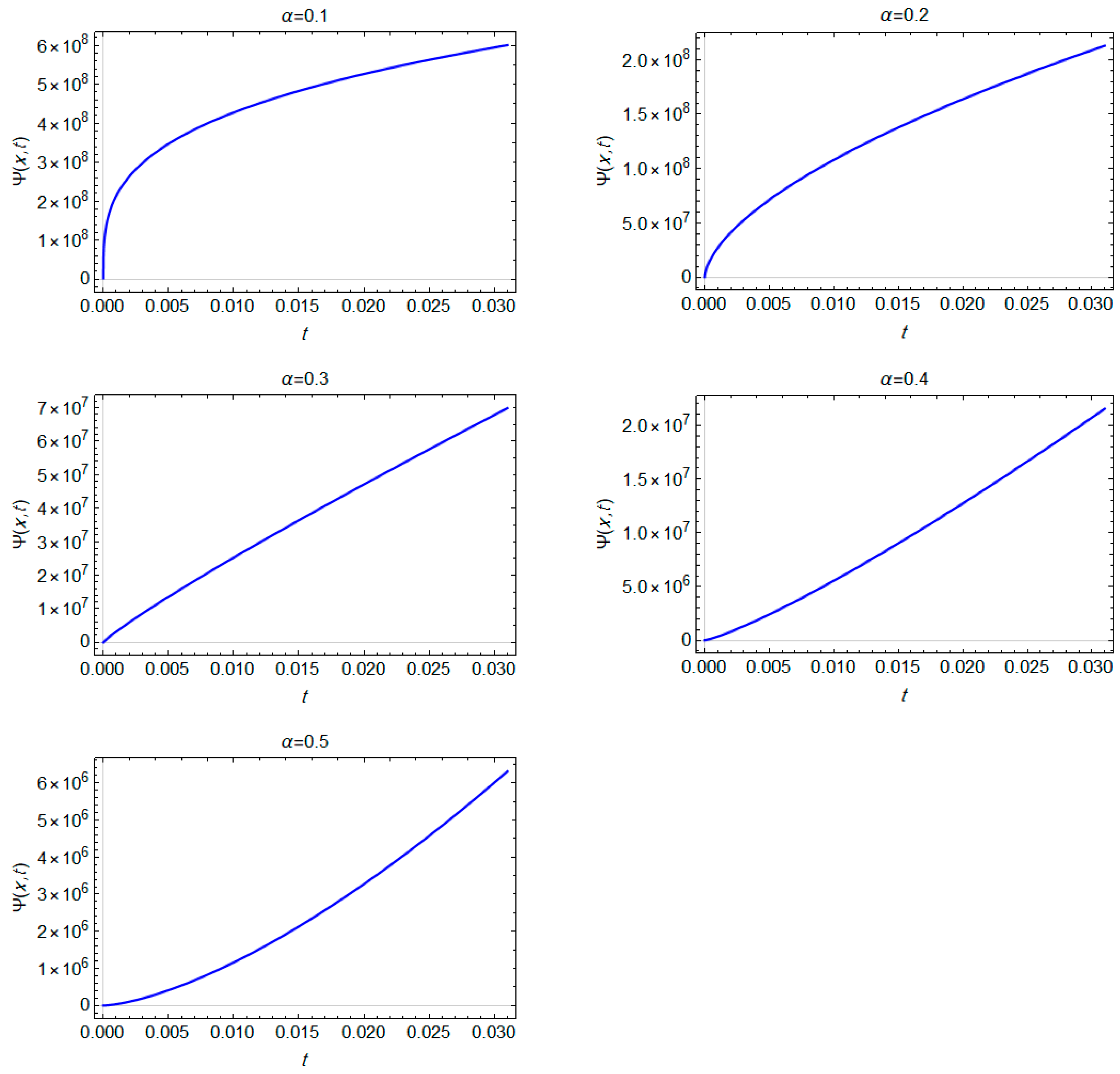
The flux was calculated at different times, and the anomalous diffusion, $\alpha <1$ (sub diffusion) was considered. Additionally, it is clear from Table 1 that the neutron flux increased with time, as shown in Figure 1.

For more clarification, the neutron fluxes $\psi \left(x,t\right)$ are plotted in Figure 1 with the initial condition ${\psi }_0\left(x\right)=x^2$.

Now, the different initial value problem $\psi \left(x,0\right)=x^2$ was used in the study of the following case, where the results are clarified in Figure 2.

The plotted profile of the neutron fluxes for different values of $\alpha$ ($\alpha =0.1, 0.2,$ 0.3, 0.4 and $\alpha =0.5$) in both cases $\{\psi \left(x,0\right)=1$ and $\psi \left(x,0\right)=x^2 \}$, as presented in Table 1 and Figure 1 and Figure 2, shows that the results were in agreement with the Adomian decomposition method [10].

As observed from the tables and figures, the Laplace residual power series method used to solve the time-dependent fractional neutron diffusion equations with delayed neutrons provided us with more details about the neutron flux in non-Gaussian diffusion for different selected times.

The importance of this work was manifested by uncovering the behavior of the flux in the presence of the delayed neutrons that affected them (this phenomenon is known as anomalous diffusion). This flux can be expressed mathematically by the solution of the time-dependent fractional neutron diffusion equations, as shown in Equation (42).

It must be noted that the time-dependent flux increased with time in both the studied numerical cases [9,10,12].

5. Conclusions

The Laplace residual power series method was presented efficiently by studying the coupled time-dependent fractional neutron diffusion equations with delayed neutrons to create an approximate fractional series solution, and the validity of the theoretical presentation of the method was confirmed by two different nuclear physics numerical case studies. The obtained fluxes for both cases were calculated and the anomalous diffusion, α < 1 (sub diffusion) was considered where the neutron fluxes increased with time; moreover, the results were successfully tested when they were compared with the Adomian decomposition method. The newly introduced concept of anomalous diffusion, which describes non-Gaussian diffusion, can be explained mathematically by fractional calculus using the Laplace residual power series method. It must be noted that the success of the combination of the residual power series and Laplace transformation in the proposed method has the potential for use in studying different nuclear reactor theories and other scientific phenomena.

References

1. Stacey, W.M. Nuclear Reactor Physics; John Wiley & Sons: Boston, MA, USA, 2001. [Google Scholar]
2. Duderstadt, J.J.; Hamilton, L.J. Nuclear Reactor Analysis; John Wiley & Sons: Boston, MA, USA, 1976. [Google Scholar]
3. Lamarsh, J.R. Introduction to Nuclear Engineering, 2nd ed.; Addison-Wesley: Boston, MA, USA, 1983. [Google Scholar]
4. Khasawneh, K.; Dababneh, S.; Odibat, Z. A solution of the neutron diffusion equation in hemispherical symmetry using the homotopy perturbation method. Ann. Nucl. Energy 2009, 36, 1711–1717. [Google Scholar] [CrossRef]
5. Dababneh, S.; Khasawneh, K.; Odibat, Z. An alternative solution of the neutron diffusion equation in cylindrical symmetry. Ann. Nucl. Energy 2010, 38, 1140–1143. [Google Scholar] [CrossRef]
6. Shqair, M. Solution of different geometries reflected reactors neutron diffusion equation using the homotopy perturbation method. Results Phys. 2019, 12, 61–66. [Google Scholar] [CrossRef]
7. Shqair, M. Developing a new approaching technique of homotopy perturbation method to solve two-group reflected cylindrical reactor. Results Phys. 2019, 12, 1880–1887. [Google Scholar] [CrossRef]
8. Shqair, M.; Farrag, E.; Al-Smadi, M. Solving Multi-Group Reflected Spherical Reactor System of Equations Using the Homotopy Perturbation Method. Mathematics 2022, 10, 1784. [Google Scholar] [CrossRef]
9. Vyawahare, V.; Nataraj, P. Fractional-Order Modeling of Nuclear Reactor: From Subdiffusive Neutron Transport to Control-Oriented Models; Springer Nature: Singapore, 2018. [Google Scholar]
10. Ray, S. Fractional Calculus with Applications for Nuclear Reactor Dynamics; CRC Press: Broken, NW, USA, 2016. [Google Scholar]
11. Aboanber, A.; Nahla, A.; Aljawazneh, S. Fractional two energy groups matrix representation for nuclear reactor dynamics with an external source. Ann. Nucl. Energy 2021, 153, 108062. [Google Scholar] [CrossRef]
12. Sardar, T.; Ray, S.; Bera, R. The solution of coupled fractional neutron diffusion equations with delayed neutrons. Int. J. Nuclear Energy Sci. Technol. 2010, 5, 105–133. [Google Scholar] [CrossRef]
13. Khaled, S. Exact solution of the one-dimensional neutron diffusion kinetic equation with one delayed precursor concentration in Cartesian geometry. AIMS Math. 2022, 7, 12364–12373. [Google Scholar] [CrossRef]
14. Burqan, A.; El-Ajou, A.; Saadeh, R.; Al-Smadi, M. A new efficient technique using Laplace transforms and smooth expansions to construct a series solution to the time-fractional Navier-Stokes equations. Alex. Eng. J. 2022, 61, 1069–1077. [Google Scholar] [CrossRef]
15. Sarhan, A.; Burqan, A.; Saadeh, R.; Al-Zhour, Z. Analytical Solutions of the Nonlinear Time-Fractional Coupled Boussinesq-Burger Equations Using Laplace Residual Power Series Technique. Fractal Fract. 2022, 6, 631. [Google Scholar] [CrossRef]
16. Kazem, S. Exact solution of some linear fractional differential equations by Laplace transform. Int. J. Nonlinear Sci. 2013, 16, 3–11. [Google Scholar]
17. Yavuz, M.; Özdemir, N. Numerical inverse Laplace homotopy technique for fractional heat equations. Therm. Sci. 2018, 22, 185–194. [Google Scholar] [CrossRef]
18. Wang, Q. Numerical solutions for fractional KdV–Burgers equation by Adomian decomposition method. Appl. Math. Comput. 2006, 182, 1048–1055. [Google Scholar] [CrossRef]
19. Cao, Y.; Nikan, O.; Avazzadeh, Z. A localized meshless technique for solving 2D nonlinear integro-differential equation with multi-term kernels. Appl. Numer. Math. 2023, 183, 140–156. [Google Scholar] [CrossRef]
20. Akram, T.; Abbas, M.; Ali, A. A numerical study on time fractional Fisher equation using an extended cubic B-spline approximation. J. Math. Comput. Sci. 2021, 22, 85–96. [Google Scholar] [CrossRef]
21. Oderinu, R.A.; Owolabi, J.A.; Taiwo, M. Approximate solutions of linear time-fractional differential equations. J. Math. Comput. Sci. 2023, 29, 60–72. [Google Scholar] [CrossRef]
22. Ali, A.; Abbas, M.; Akram, T. New group iterative schemes for solving the two-dimensional anomalous fractional sub-diffusion equation. J. Math. Comp. Sci. 2021, 22, 119–127. [Google Scholar] [CrossRef]
23. Liao, H.; Zhang, D.; Zhao, Y. Sharp error estimate of a nonuniform L1 formula for time-fractional reaction subdiffusion equations. SIAM J. Numer. Anal. 2018, 56, 1122–1133. [Google Scholar] [CrossRef]
24. Lyu, P.; Vong, S. A symmetric fractional-order reduction method for direct nonuniform approximations of semilinear diffusion-wave equations. J. Sci. Comput. 2022, 93, 34. [Google Scholar] [CrossRef]
25. Eriqat, T.; El-Ajou, A.; Moa’ath, N.O.; Al-Zhour, Z.; Momani, S. A new attractive analytic approach for solutions of linear and nonlinear neutral fractional pantograph equations. Chaos Solitons Fractals 2020, 138, 109957. [Google Scholar] [CrossRef]
26. Oldham, K.; Spanier, J. The Fractional Calculus Theory and Applications of Differentiation and Integration to Arbitrary Order, 1st ed.; Elsevier: Amsterdam, The Netherlands, 1974. [Google Scholar]
Figure 1. Two-dimensional graphs of neutron flux ψ x ,   t for α = 0.1, 0.2, 0.3, 0.4, and 0.5 (colored online).
Fractalfract 07 00219 g001
Figure 2. Three-dimensional graphs of neutron flux ψ x ,   t with ψ 0 x = x 2 for α = 0.1, 0.2, 0.3, 0.4 and 0.5 (colored online). Two-dimensional graphs of neutron flux ψ x ,   t for α = 0.1, 0.2, 0.3, 0.4, and 0.5 (colored online).
Fractalfract 07 00219 g002