
A Visually Secure Image Encryption Based on the Fractional Lorenz System and Compressive Sensing


Abstract
:1. Introduction
2. Preliminaries
2.1. Compressive Sensing
2.2. The 3D Fractional Lorenz System
2.3. Vector Quantization
3. The Proposed Scheme
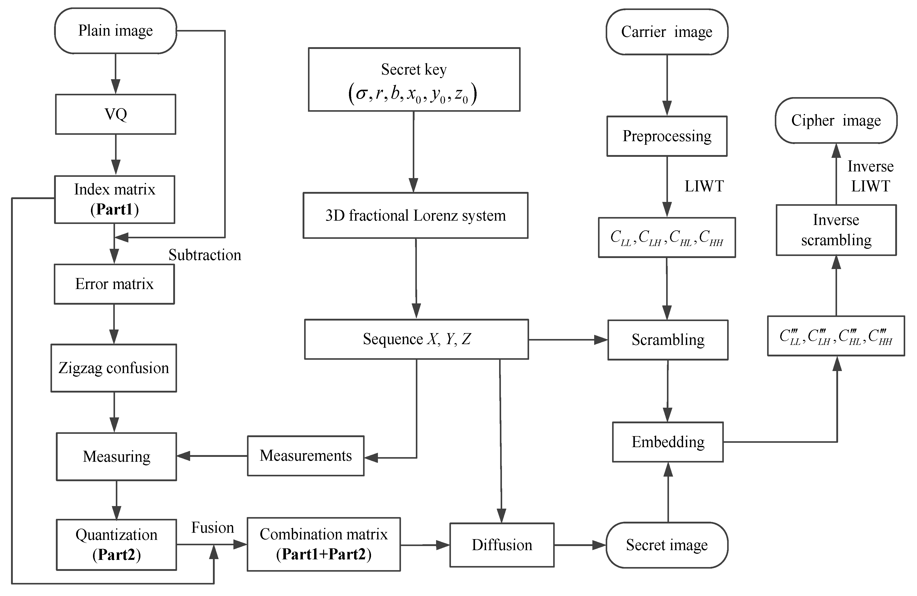
3.1. Encryption Process
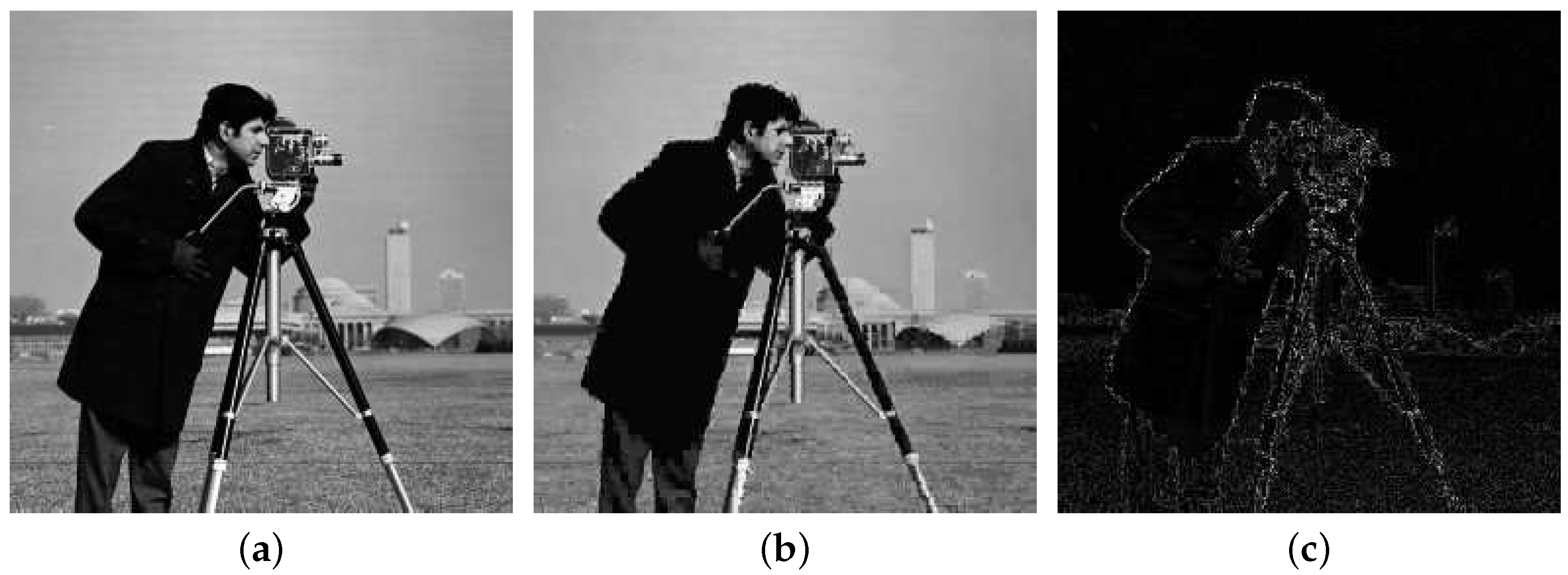
3.1.1. Generating Index Matrix and Error Matrix Based on VQ
3.1.2. Generating the Secret Image Based on CS and Zigzag Confusion
| Algorithm 1: The construction of measurement matrix . |
Input: A distance d, the initial values , and control parameters . Output: The measurement matrix . (1): Iterate the 3D Lorenz system times with initial values and control parameters , abandon the preceding elements to bypass the transient state, then obtain three chaotic secret code streams , and . (2): Obtain the sequence based on . (3): Generate the sequence by sampling sequence with interval d as . (4): Obtain a more random sequence with . (5): Construct the measurement matrix according to the following formula: |
3.1.3. Embedding the Secret Image into the Carrier Image
| Algorithm 2: The embedding process. |
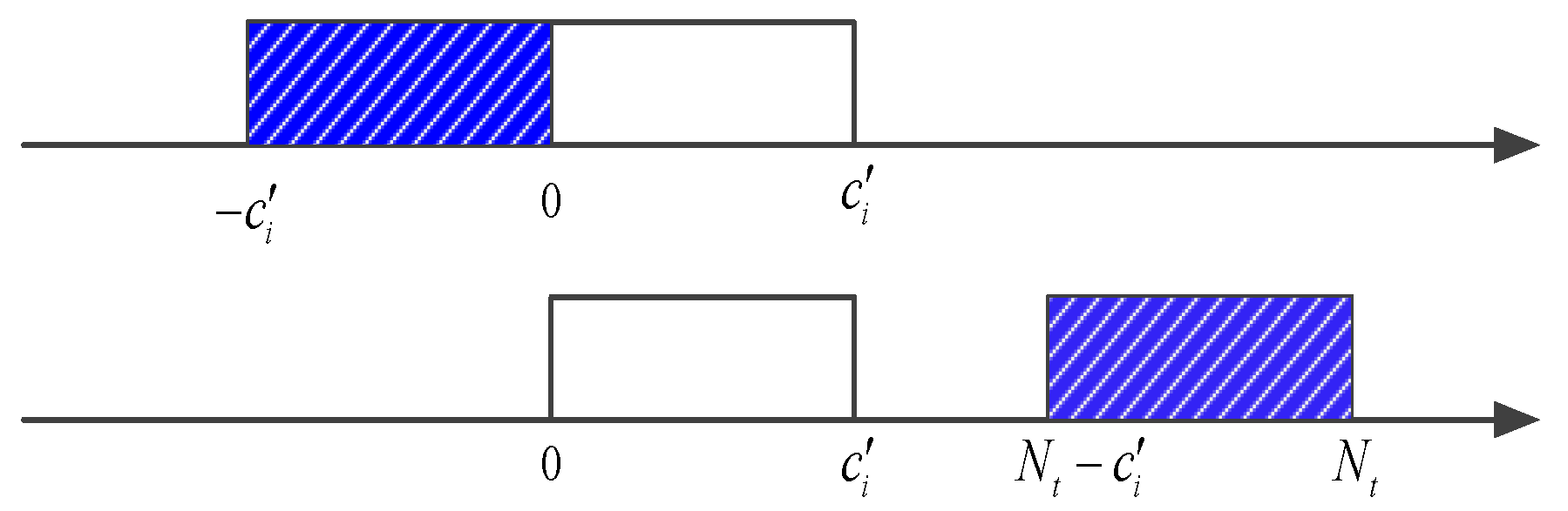
Input: The secret image and the scrambled components , , and . Output: The marked coefficient components , , and . (1): Stretch the secret image into a one-dimensional vector , and represent all the elements of the vector in binary as , where is the highest bit and is the lowest bit. (2): Quantify the coefficients of , , and into non-negative integers in a reversible way.
(3): Use the smooth function to embed and into the lowest three bits of the components and , respectively. The embedding process for is described as the following formula: (4): Embed into the lowest two bits of directly and keep other higher bits constant, then obtain the marked coefficient matrix . |
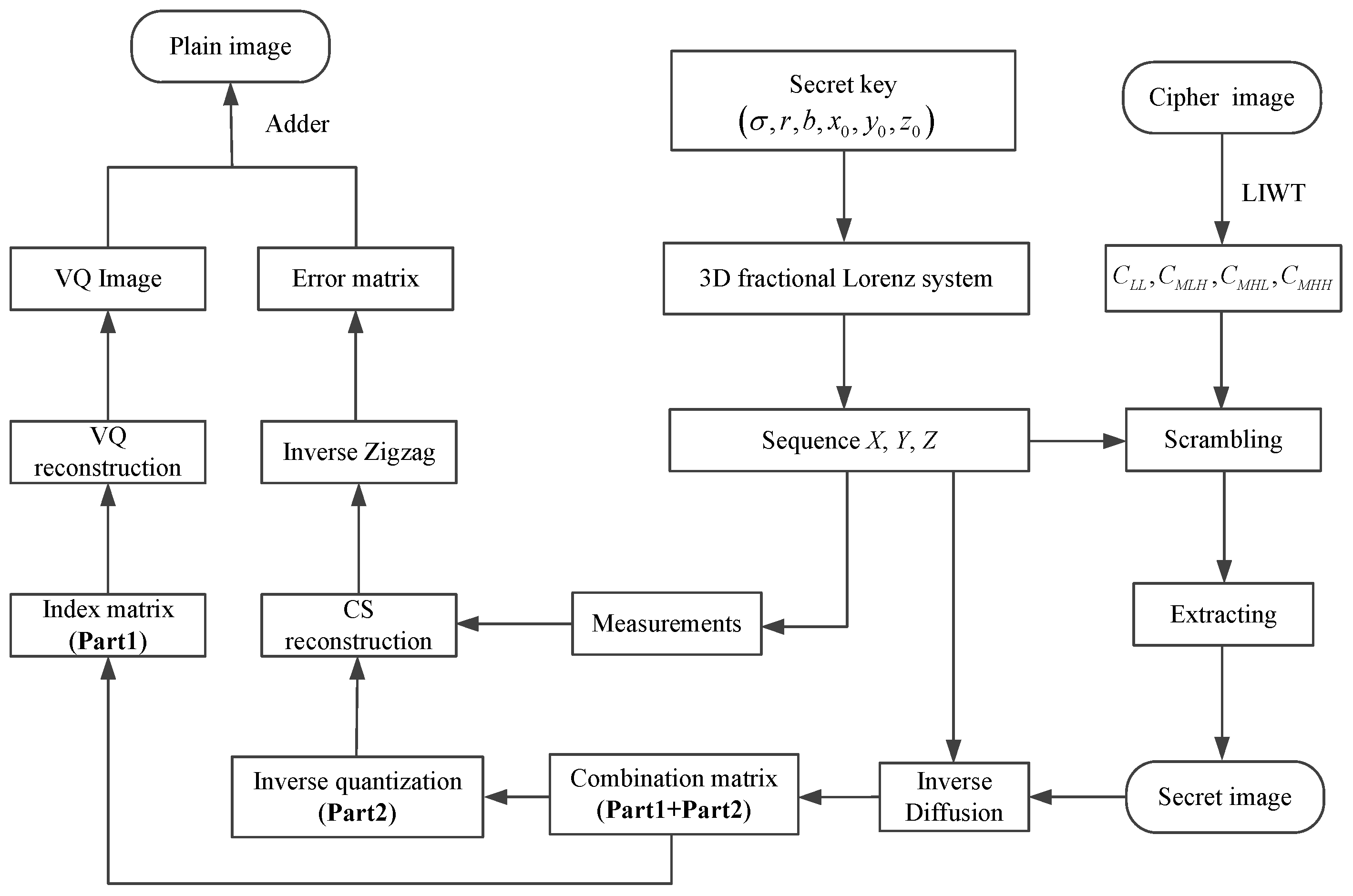
3.2. Decryption Process
3.2.1. Extracting the Secret Image from the Cipher Image
3.2.2. Recovering the Plain Image
4. Simulation and Performance Analyses
4.1. Simulation Results
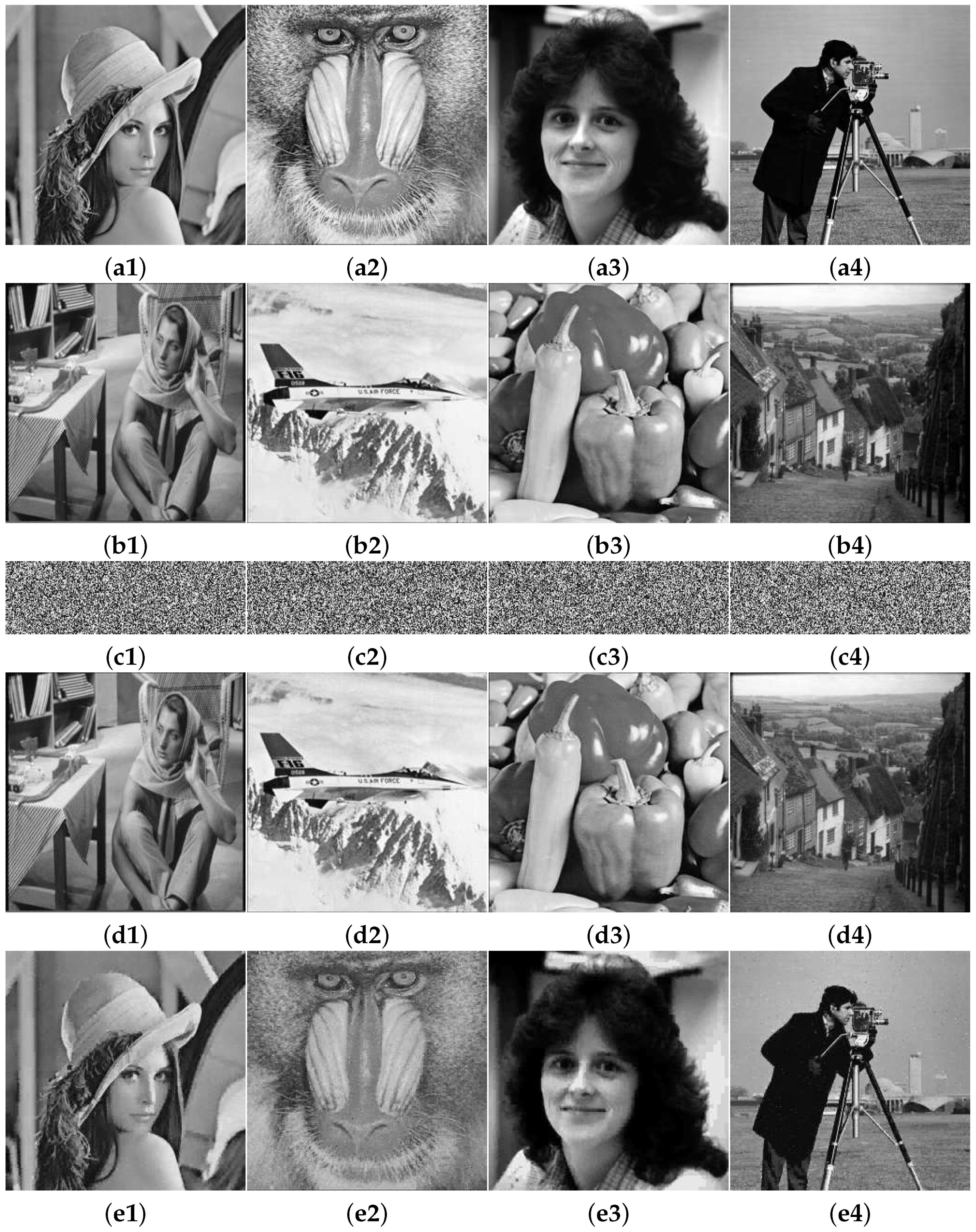
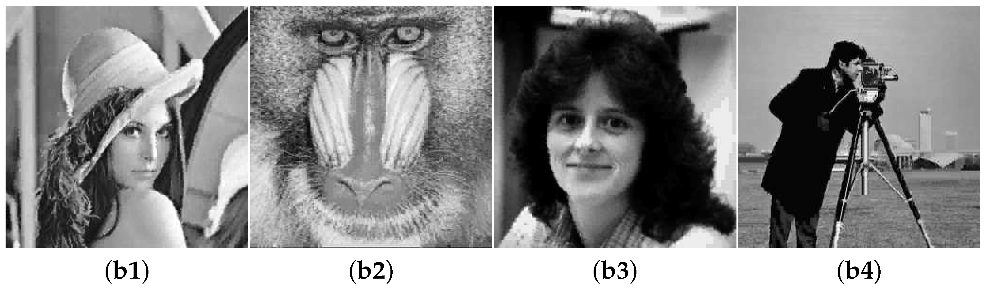
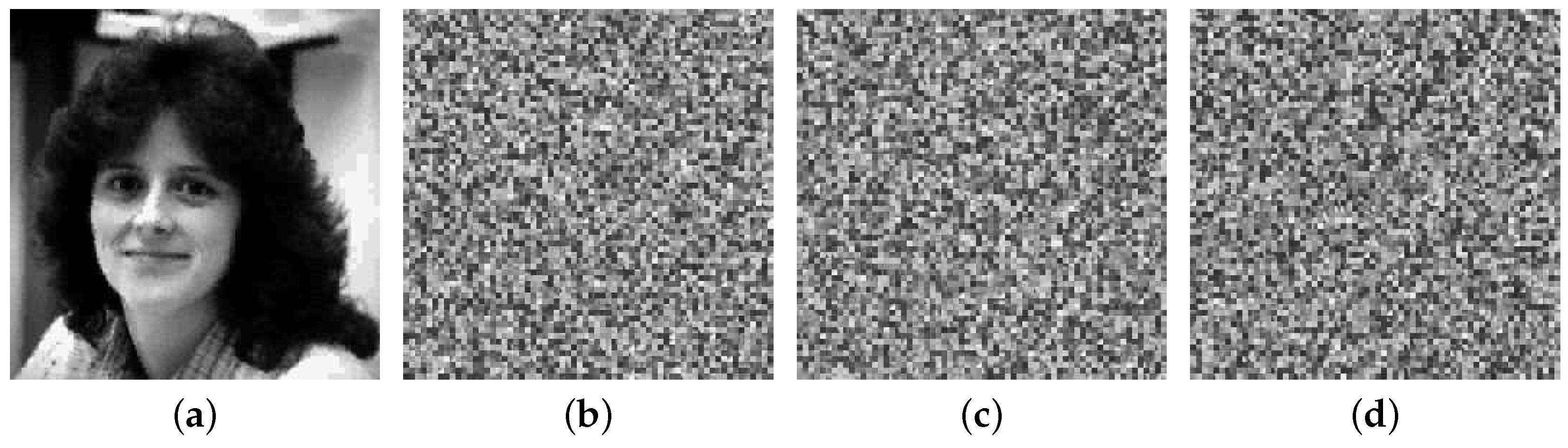
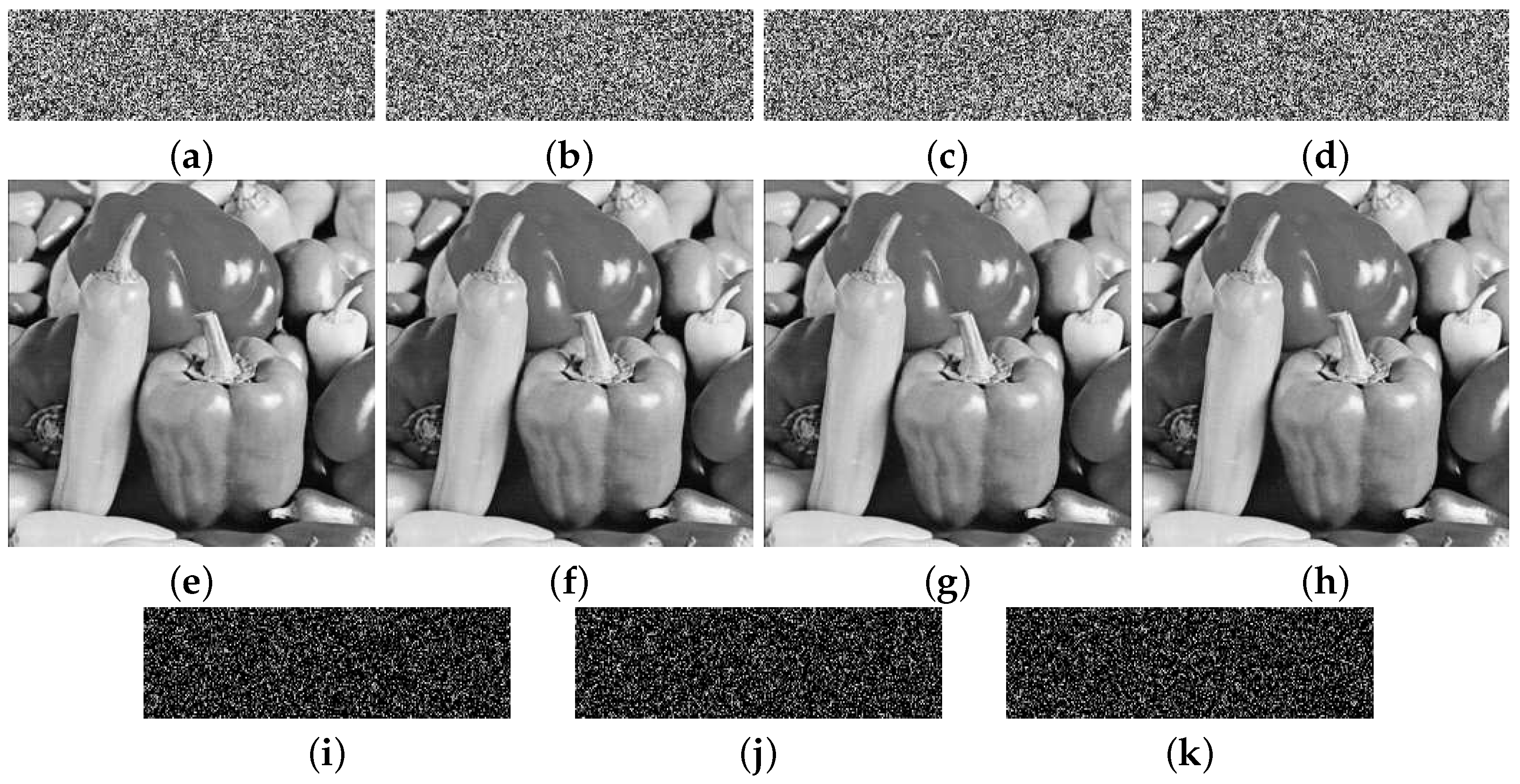
4.1.1. Encryption and Decryption Results
4.1.2. Influence of Different Carrier Images on Encryption and Decryption
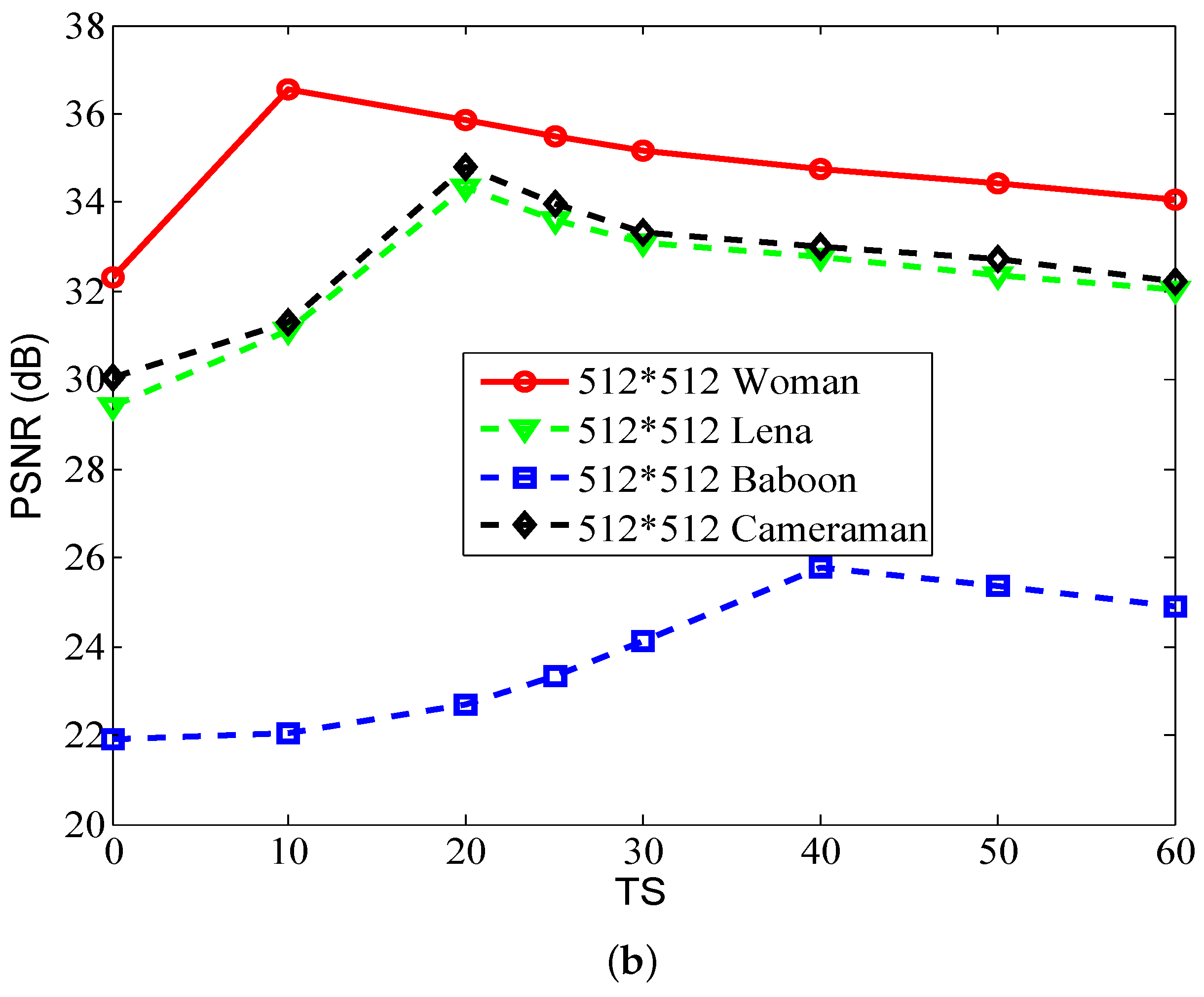
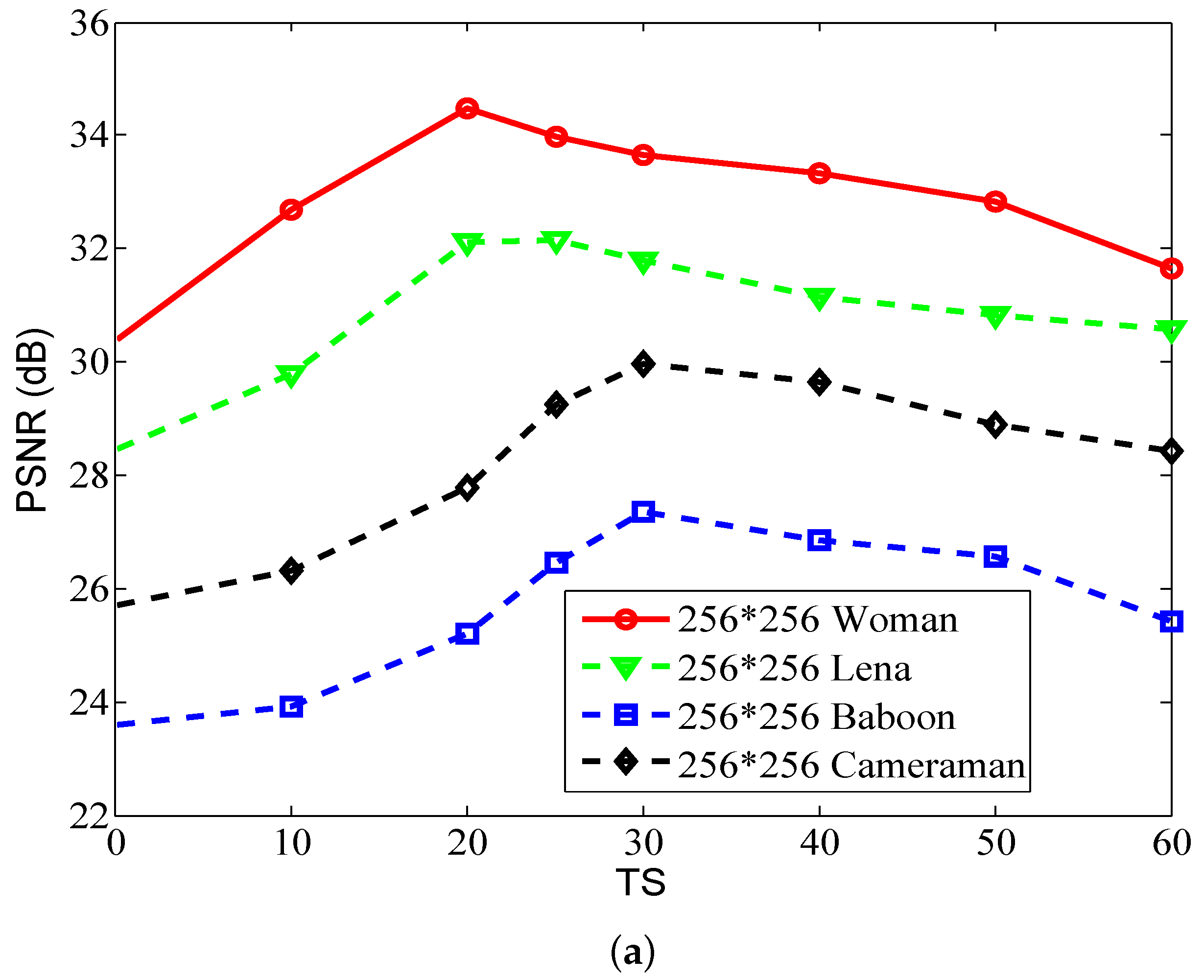
4.1.3. Influence of Threshold TS on Encryption and Decryption
4.2. Performance Analyses
4.2.1. Key Space and Sensitive Analysis
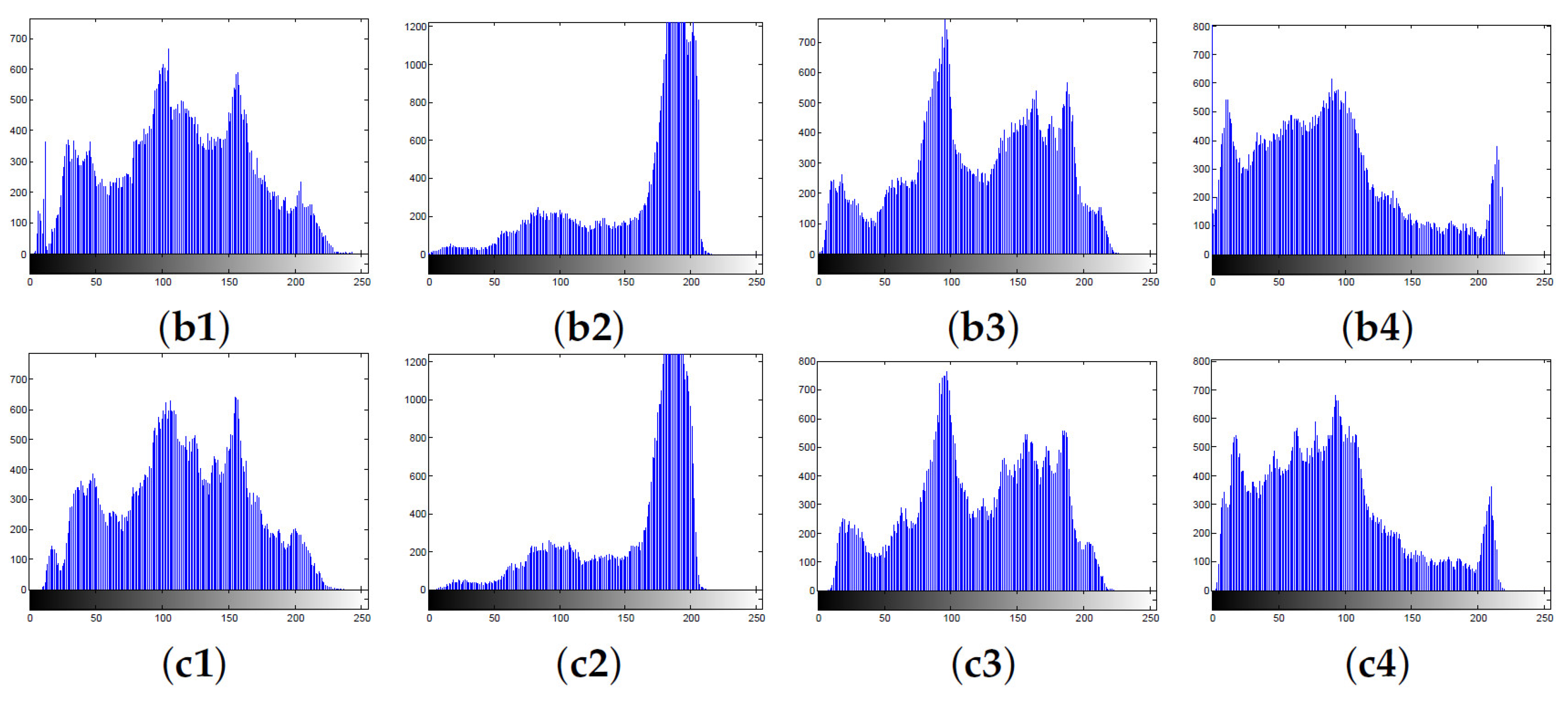
4.2.2. Histogram Analysis
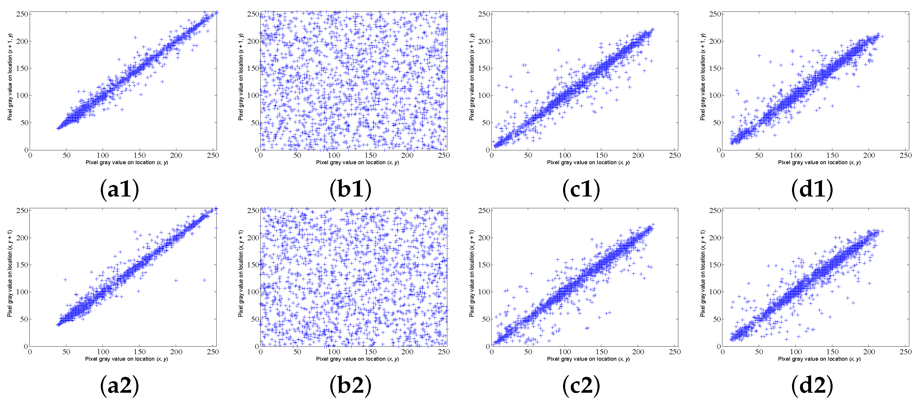
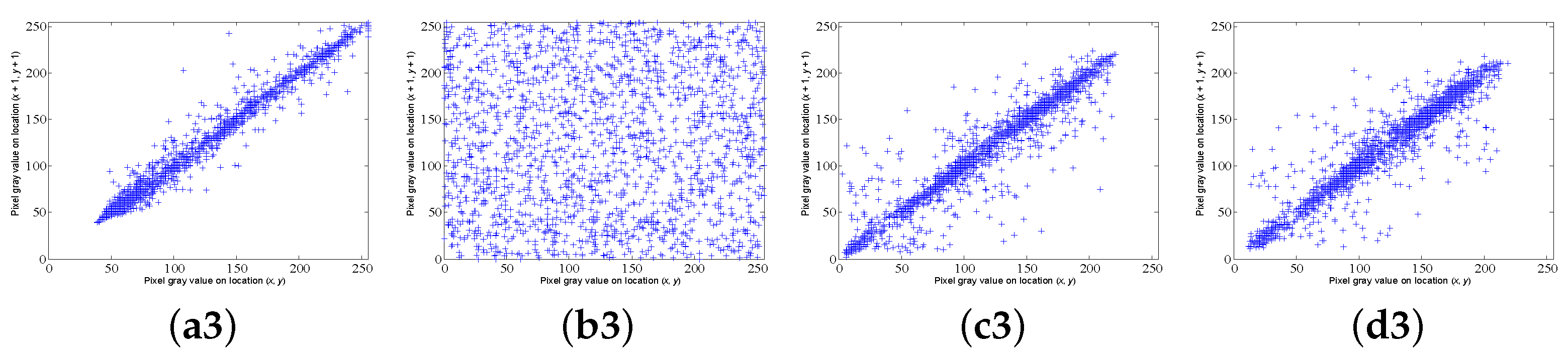
4.2.3. Correlation Analysis
4.2.4. Information Entropy Analysis
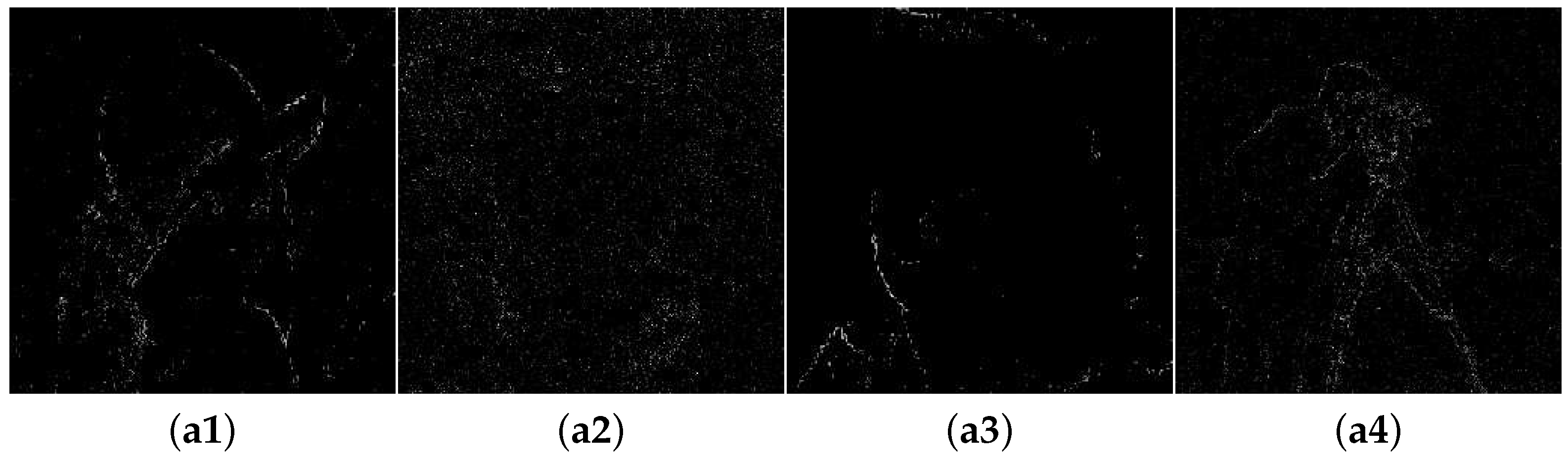
4.2.5. Cpa Attack
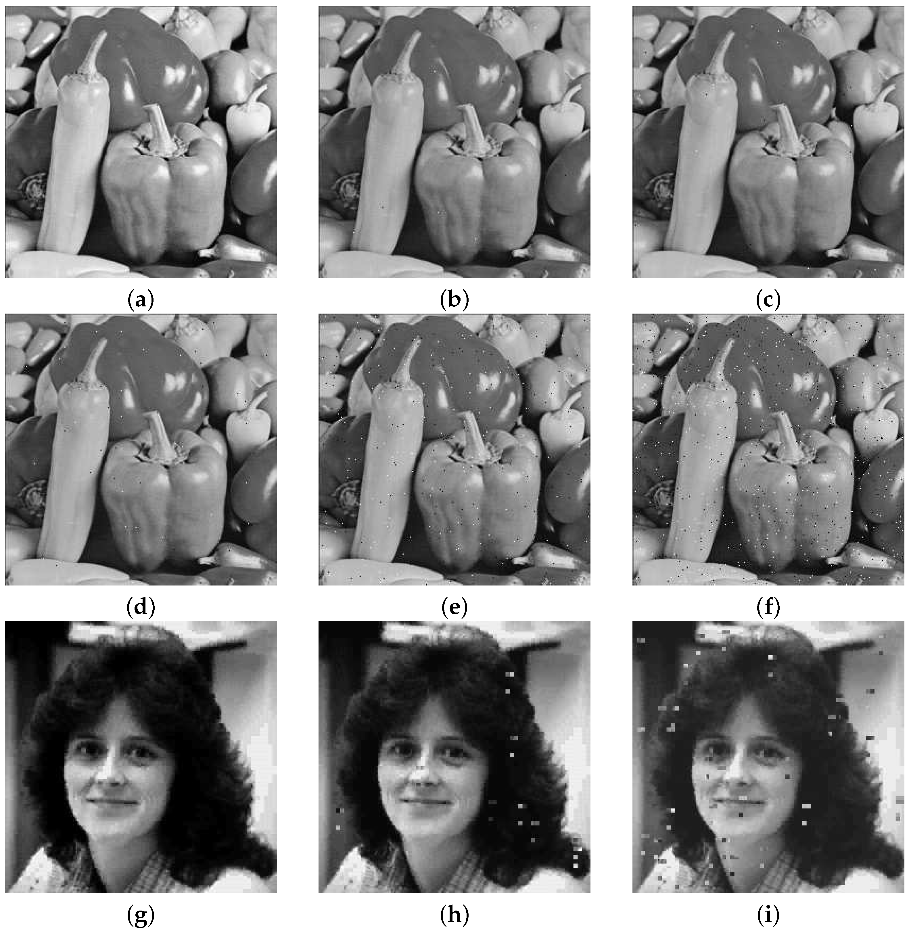
4.2.6. Noise Attack
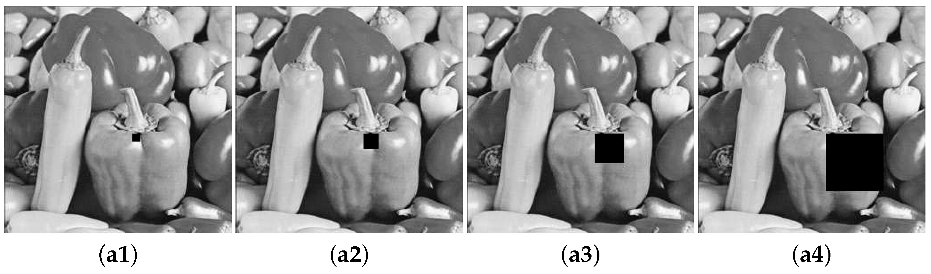
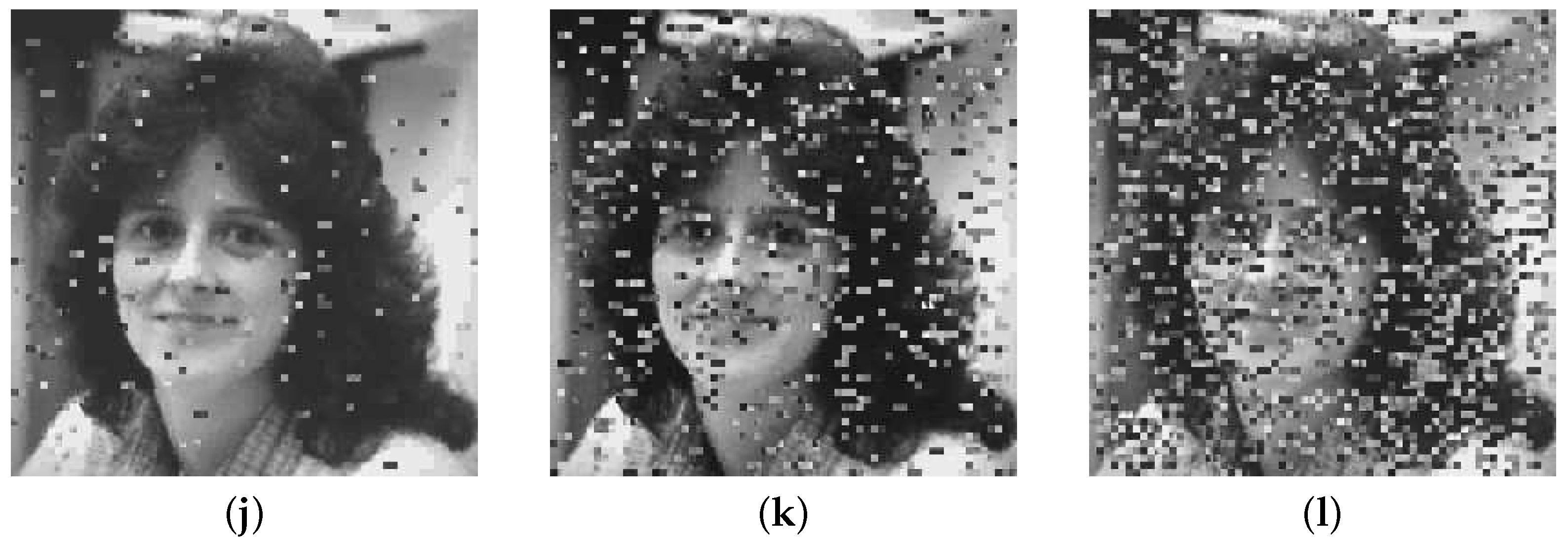
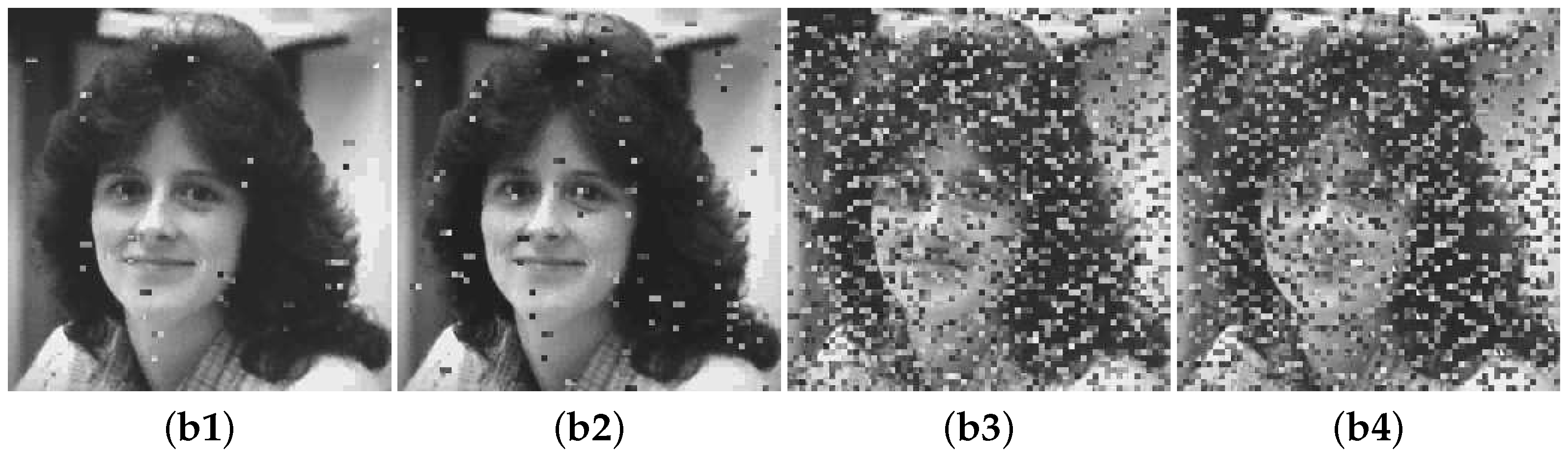
4.2.7. Data Loss Attack
4.2.8. Running Efficiency Analysis
4.3. Comparison with the Existing Work
4.3.1. Visual Security
4.3.2. Compression Performance
5. Conclusions
Author Contributions
Funding
Institutional Review Board Statement
Informed Consent Statement
Data Availability Statement
Acknowledgments
Conflicts of Interest
References
- Zhang, J.; Bhuiyan, M.; Yang, X.; Singh, A.; Hsu, D.; Luo, E. Trustworthy Tarobtain Tracking with Collaborative Deep Reinforcement Learning in EdgeAI-Aided IoT. IEEE Trans Ind. Inf. 2022, 18, 1301–1309. [Google Scholar] [CrossRef]
- Zhang, J.; Bhuiyan, M.; Yang, X.; Wang, T.; Hayajneh, T.; Xu, X. Reliable Detection of Adversary Concealed Behaviors in EdgeAI Assisted IoT. IEEE Internet Things J. 2022, 1–10. [Google Scholar] [CrossRef]
- Chen, J.; Zhu, Z.; Fu, C.; Zhang, L.; Zhang, Y. An efficient image encryption scheme using lookup table-based confusion and diffusion. Nonlinear Dyn. 2015, 81, 1151–1161. [Google Scholar] [CrossRef]
- Wu, G.; Baleanu, D.; Lin, Z. Image encryption technique based on fractional chaotic time series. J. Vib. Control 2016, 22, 2092–2099. [Google Scholar] [CrossRef]
- Zhou, N.; Yan, X.; Liang, H.; Tao, X.; Li, G. Multi-image encryption scheme based on quantum 3D Arnold transform and scaled Zhongtang chaotic system. Quantum Inf. Process. 2018, 17, 338. [Google Scholar] [CrossRef]
- Patel, S.; Vaish, A. A novel image coding through the chaos theory and compressed sensing. In Proceedings of the International Conference on Data Science and Applications, Kolkata, India, 26–27 March 2022; Volume 287, pp. 615–623. [Google Scholar]
- Lu, P.; Xu, Z.; Lu, X.; Liu, X. Digital image information encryption based on Compressive Sensing and double random-phase encoding technique. Optik 2013, 124, 2514–2518. [Google Scholar] [CrossRef]
- Patel, S.; Vaish, A. A systematic survey on Image Encryption using Compressive Sensing. J. Sci. Res. 2020, 64, 391–396. [Google Scholar] [CrossRef]
- Vaish, A.; Patel, S. A sparse representation based compression of fused images using WDR coding. J. King. Saud. Univ.-Comput. Inf. Sci. 2022, in press. [Google Scholar] [CrossRef]
- Wang, Z.; Huang, X.; Li, Y.; Song, X. A new image encryption algorithm based on the fractional-order hyperchaotic Lorenz system. Chin. Phys. B 2013, 22, 010504. [Google Scholar] [CrossRef]
- He, J.; Yu, S.; Cai, J. A method for image encryption based on fractional-order hyperchaotic systems. J. Appl. Anal. Comput. 2015, 5, 197–209. [Google Scholar]
- Badr, I.; Radwan, A.; El-Rabaie, E.; Said, L.; El Banby, G.; El-Shafai, W.; Abd El-Samie, F. Cancellable face recognition based on fractional-order Lorenz chaotic system and Haar wavelet fusion. Digit. Signal Process. 2021, 116, 103103. [Google Scholar] [CrossRef]
- Yang, Y.; Guan, B.; Li, J.; Li, D.; Zhou, Y.; Shi, W. Image compression-encryption scheme based on fractional order hyper-chaotic systems combined with 2D compressed sensing and DNA encoding. Opt. Laser Technol. 2019, 119, 105661. [Google Scholar] [CrossRef]
- Kayalvizhi, S.; Malarvizhi, S. A novel encrypted compressive sensing of images based on fractional order hyper chaotic Chen system and DNA operations. Multimed. Tools Appl. 2020, 79, 3957–3974. [Google Scholar] [CrossRef]
- Fan, H.; Zhou, K.; Zhang, E.; Wen, W.; Li, M. Subdata image encryption scheme based on compressive sensing and vector quantization. Neural Comput. Appl. 2020, 1, 1–17. [Google Scholar] [CrossRef]
- Ye, H.; Dai, J.; Wen, S.; Gong, L.; Zhang, W. Color image encryption scheme based on quaternion discrete multi-fractional random transform and compressive sensing. Opt. Appl. 2021, 51, 349–364. [Google Scholar]
- Bao, L.; Zhou, Y. Image encryption: Generating visually meaningful encrypted images. Inf. Sci. 2015, 324, 197–207. [Google Scholar] [CrossRef]
- Musanna, F.; Kumar, S. Generating visually coherent encrypted images with reversible data hiding in wavelet domain by fusing chaos and pairing function. Comput. Commun. 2020, 162, 12–30. [Google Scholar] [CrossRef]
- Chai, X.; Gan, Z.; Chen, Y.; Zhang, Y. A visually secure image encryption scheme based on compressive sensing. Signal Process. 2017, 134, 35–51. [Google Scholar] [CrossRef] [Green Version]
- Wang, H.; Xiao, D.; Li, M.; Xiang, Y.; Li, X. A visually secure image encryption scheme based on parallel compressive sensing. Signal Process. 2019, 155, 218–232. [Google Scholar] [CrossRef]
- Chai, X.; Wu, H.; Gan, Z.; Zhang, Y.; Chen, Y.; Kent, W. An efficient visually meaningful image compression and encryption scheme based on compressive sensing and dynamic LSB embedding. Opt. Laser Eng. 2020, 124, 105837. [Google Scholar] [CrossRef]
- Wen, W.; Hong, Y.; Fang, Y.; Li, M.; Li, M. A visually secure image encryption scheme based on semi-tensor product compressed sensing. Signal Process. 2020, 173, 107580. [Google Scholar] [CrossRef]
- Ping, P.; Yang, X.; Zhang, X.; Mao, Y.; Khalid, H. Generating visually secure encrypted images by partial block pairing-substitution and semi-tensor product compressed sensing. Digit. Signal Process. 2022, 120, 103263. [Google Scholar] [CrossRef]
- Zhu, L.; Song, H.; Zhang, X.; Yan, M.; Zhang, T.; Wang, X.; Xu, J. A robust meaningful image encryption scheme based on block compressive sensing and SVD embedding. Signal Process. 2020, 175, 107629. [Google Scholar] [CrossRef]
- Wang, X.; Ren, Q.; Jiang, D. An adjustable visual image cryptosystem based on 6D hyperchaotic system and compressive sensing. Nonlinear Dyn. 2021, 104, 4543–4567. [Google Scholar] [CrossRef]
- Chai, X.; Wu, H.; Gan, Z.; Han, D.; Zhang, Y.; Chen, Y. An efficient approach for encrypting double color images into a visually meaningful cipher image using 2D compressive sensing. Inf. Sci. 2021, 556, 305–340. [Google Scholar] [CrossRef]
- Huo, D.; Zhu, Z.; Wei, L.; Han, C.; Zhou, X. A visually secure image encryption scheme based on 2D compressive sensing and integer wavelet transform embedding. Opt. Commun. 2021, 492, 126976. [Google Scholar] [CrossRef]
- Wang, K.; Liu, M.; Zhang, Z.; Gao, T. Optimized visually meaningful image embedding strategy based on compressive sensing and 2D DWT-SVD. Multimed Tools Appl. 2022, 81, 20175–20199. [Google Scholar] [CrossRef]
- Lee, T.; Lin, S. Dual watermark for image tamper detection and recovery. Pattern Recogn. 2008, 41, 3497–3506. [Google Scholar] [CrossRef]
- Zheng, P.; Huang, J. Discrete wavelet transform and data expansion reduction in homomorphic encrypted domain. IEEE Trans. Image Process. 2013, 22, 2455–2468. [Google Scholar] [CrossRef]
- Yang, S.; Chen, C.; Yau, H. Control of chaos in Lorenz system. Chaos Soliton. Fract. 2002, 13, 767–780. [Google Scholar] [CrossRef]
- Wang, S.; Wu, R. Dynamic analysis of a 5D fractional-order hyperchaotic system. Int. J. Control Autom. Syst. 2017, 15, 1003–1010. [Google Scholar] [CrossRef]
- Linde, Y.; Buzo, A.; Gray, R. An algorithm for vector quantizer design. IEEE Trans. Commun. 1980, 28, 84–95. [Google Scholar] [CrossRef] [Green Version]
- Wang, Z.; Bovik, A.; Sheikh, H.; Simoncelli, E. Image quality assessment: From error visibility to structural similarity. IEEE Trans. Image Process. 2004, 13, 600–612. [Google Scholar] [CrossRef] [PubMed] [Green Version]
- Alvarez, G.; Li, S. Some basic cryptographic requirements for chaos-based cryptosystems. Int. J. Bifurc. Chaos 2006, 16, 2129–2151. [Google Scholar] [CrossRef] [Green Version]
- Murillo-Escobar, M.; Meranza-Castillón, M.; López-Gutiérrez, R.; Cruz-Hernandez, C. Suggested integral analysis for chaos-based image cryptosystems. Entropy 2019, 21, 815. [Google Scholar] [CrossRef] [PubMed] [Green Version]


| Size | Plain Image | Carrier Image | With Smooth Function | Without Smooth Function | ||||
|---|---|---|---|---|---|---|---|---|
| PSNRdec(dB) | PSNRciph(dB) | MSSIMciph | PSNRdec(dB) | PSNRciph(dB) | MSSIMciph | |||
| Lena | Barbara | 32.1670 | 42.3844 | 0.9990 | 32.1670 | 39.7819 | 0.9982 | |
| Baboon | Jet | 26.4461 | 42.4317 | 0.9978 | 26.4461 | 39.4862 | 0.9960 | |
| Woman | Peppers | 33.9596 | 42.4443 | 0.9983 | 33.9596 | 39.7859 | 0.9970 | |
| Cameraman | Goldhill | 29.2672 | 42.3324 | 0.9986 | 29.2672 | 39.6536 | 0.9976 | |
| Lena | Barbara | 33.6028 | 42.3879 | 0.9985 | 33.9741 | 39.6025 | 0.9974 | |
| Baboon | Jet | 23.3306 | 42.4855 | 0.9972 | 23.3306 | 39.5200 | 0.9952 | |
| Woman | Peppers | 35.4988 | 42.3948 | 0.9976 | 35.4988 | 39.7142 | 0.9958 | |
| Cameraman | Goldhill | 33.9741 | 42.3654 | 0.9981 | 33.6028 | 39.7277 | 0.9968 | |
| Plain Image | Carrier Image | With Smooth Function | Without Smooth Function | ||||
|---|---|---|---|---|---|---|---|
| PSNRdec(dB) | PSNRciph(dB) | MSSIMciph | PSNRdec(dB) | PSNRciph(dB) | MSSIMciph | ||
| Woman () | Barbara | 33.9596 | 42.3844 | 0.9990 | 33.9596 | 39.7819 | 0.9982 |
| Jet | 33.7542 | 42.4317 | 0.9978 | 33.7542 | 39.4862 | 0.9960 | |
| Lena | 33.4563 | 42.5292 | 0.9981 | 33.4563 | 39.6842 | 0.9978 | |
| Goldhill | 33.6521 | 42.3324 | 0.9986 | 33.6521 | 39.6536 | 0.9976 | |
| Woman () | Barbara | 35.4988 | 42.3879 | 0.9985 | 35.4988 | 39.6025 | 0.9974 |
| Jet | 35.4356 | 42.4855 | 0.9972 | 35.4356 | 39.5200 | 0.9952 | |
| Lena | 35.4732 | 42.4021 | 0.9977 | 35.4732 | 39.7345 | 0.9961 | |
| Goldhill | 35.4381 | 42.3654 | 0.9981 | 35.4381 | 39.7277 | 0.9968 | |
| Image | Horizontal | Vertical | Diagonal |
|---|---|---|---|
| Plain image | 0.9915 | 0.9935 | 0.9863 |
| Secret image | 0.0287 | −0.0056 | −0.0536 |
| Carrier image | 0.9694 | 0.9754 | 0.9435 |
| Cipher image | 0.9676 | 0.9676 | 0.9305 |
| Image | Plain Image | Secret Image | Carrier Image | Cipher Image |
|---|---|---|---|---|
| Baboon | 7.1391 | 7.9896 | 7.2185 | 7.1396 |
| Woman | 7.2695 | 7.9895 | 7.2185 | 7.1396 |
| Cameraman | 7.0477 | 7.9899 | 7.2185 | 7.1398 |
| Jet | 6.7059 | 7.9901 | 7.2185 | 7.1399 |
| Peppers | 7.5924 | 7.9890 | 7.2185 | 7.1395 |
| Barbara | 7.6385 | 7.9894 | 7.2185 | 7.1395 |
| Image | Noise Intensity | |||||
|---|---|---|---|---|---|---|
| 0.00001 | 0.0001 | 0.0005 | 0.001 | 0.005 | 0.01 | |
| Woman () | 41.0635 | 40.8181 | 39.2176 | 34.5001 | 28.2351 | 25.4084 |
| Peppers () | 32.5193 | 29.3239 | 28.6176 | 22.3247 | 15.9286 | 14.1350 |
| Size of Data Loss | PSNR (dB) | MSSIM | CC |
|---|---|---|---|
| 28.9935 | 0.9477 | 0.9891 | |
| 24.8029 | 0.8661 | 0.9714 | |
| 18.6750 | 0.6018 | 0.8828 | |
| 14.2427 | 0.3748 | 0.6503 |
| Item | Lena | Baboon | Woman | Cameraman | Average |
|---|---|---|---|---|---|
| Compression | 0.1405 | 0.1256 | 0.1200 | 0.1324 | 0.1296 |
| Diffusion | 0.0057 | 0.0074 | 0.0100 | 0.0062 | 0.0073 |
| Embedding | 16.9714 | 17.3376 | 17.8024 | 16.9080 | 17.2549 |
| Total | 5.7059 | 5.8235 | 5.9775 | 5.6822 | 5.7973 |
| Item | Lena | Baboon | Woman | Cameraman | Average |
|---|---|---|---|---|---|
| Extraction | 8.5617 | 8.6331 | 8.9388 | 8.6678 | 8.7004 |
| Inverse-diffusion | 0.0049 | 0.0054 | 0.0059 | 0.0052 | 0.0054 |
| Reconstruction | 6.6999 | 6.8180 | 7.0726 | 6.5937 | 6.7961 |
| Total | 5.0888 | 5.1522 | 5.3391 | 5.0889 | 5.1673 |
| Item | Lena | Baboon | Woman | Cameraman | Average |
|---|---|---|---|---|---|
| Compression | 0.7345 | 0.7897 | 0.7124 | 0.7345 | 0.7428 |
| Diffusion | 0.0106 | 0.0096 | 0.0103 | 0.0100 | 0.0101 |
| Embedding | 69.0720 | 68.7851 | 69.6957 | 70.4789 | 69.5079 |
| Total | 23.2724 | 23.1948 | 23.4728 | 23.7411 | 23.4203 |
| Item | Lena | Baboon | Woman | Cameraman | Average |
|---|---|---|---|---|---|
| Extraction | 34.5340 | 35.4738 | 35.5933 | 34.6818 | 35.0707 |
| Inverse-diffusion | 0.0089 | 0.0116 | 0.0092 | 0.0089 | 0.0097 |
| Reconstruction | 27.5058 | 28.4689 | 27.7533 | 27.1136 | 27.7104 |
| Total | 20.6829 | 21.3181 | 21.1186 | 20.6014 | 20.9303 |
| Plain Image | Carrier Image | PSNR (dB) | MSSIM | ||||||
|---|---|---|---|---|---|---|---|---|---|
| Ref. [19] | Ref. [20] | Ref. [24] | Ours | Ref. [19] | Ref. [20] | Ref. [24] | Ours | ||
| Lena | Peppers | 18.5136 | 32.3513 | 31.7986 | 42.4468 | 0.6726 | 0.9257 | 0.9903 | 0.9983 |
| Jet | Baboon | 23.3967 | 37.1058 | 32.5976 | 42.2459 | 0.6991 | 0.9833 | 0.9955 | 0.9989 |
| Girl | Goldhill | 28.2318 | 36.1125 | 32.0647 | 42.1456 | 0.7021 | 0.9666 | 0.9942 | 0.9986 |
| Barbara | Bridge | 25.2321 | 35.5629 | 31.7397 | 42.2451 | 0.7337 | 0.9783 | 0.9946 | 0.9993 |
| Average | 23.8436 | 35.2831 | 32.0502 | 42.2709 | 0.7019 | 0.9635 | 0.9937 | 0.9988 | |
| Plain Image | Carrier Image | Ref. [19] | Ref. [20] | Ref. [21] | Ours | |
|---|---|---|---|---|---|---|
| Barbara () | Lena () | PSNR (dB) | 28.4817 | 28.4435 | 28.5534 | 29.3547 |
| MSSIM | 0.9915 | 0.8128 | 0.9932 | 0.9920 | ||
| Bridge () | PSNR (dB) | 28.1745 | 28.4435 | 28.5534 | 29.7569 | |
| MSSIM | 0.9865 | 0.8128 | 0.9932 | 0.9920 | ||
| Girl () | PSNR (dB) | 28.1932 | 28.4435 | 28.5534 | 29.4532 | |
| MSSIM | 0.9872 | 0.8128 | 0.9932 | 0.9920 | ||
| Peppers () | PSNR (dB) | 28.2321 | 28.4435 | 28.5534 | 29.5542 | |
| MSSIM | 0.9891 | 0.8128 | 0.9932 | 0.9920 |
Publisher’s Note: MDPI stays neutral with regard to jurisdictional claims in published maps and institutional affiliations. |
© 2022 by the authors. Licensee MDPI, Basel, Switzerland. This article is an open access article distributed under the terms and conditions of the Creative Commons Attribution (CC BY) license (https://creativecommons.org/licenses/by/4.0/).
Share and Cite
Ren, H.; Niu, S.; Chen, J.; Li, M.; Yue, Z. A Visually Secure Image Encryption Based on the Fractional Lorenz System and Compressive Sensing. Fractal Fract. 2022, 6, 302. https://doi.org/10.3390/fractalfract6060302
Ren H, Niu S, Chen J, Li M, Yue Z. A Visually Secure Image Encryption Based on the Fractional Lorenz System and Compressive Sensing. Fractal and Fractional. 2022; 6(6):302. https://doi.org/10.3390/fractalfract6060302
Chicago/Turabian StyleRen, Hua, Shaozhang Niu, Jiajun Chen, Ming Li, and Zhen Yue. 2022. "A Visually Secure Image Encryption Based on the Fractional Lorenz System and Compressive Sensing" Fractal and Fractional 6, no. 6: 302. https://doi.org/10.3390/fractalfract6060302
APA StyleRen, H., Niu, S., Chen, J., Li, M., & Yue, Z. (2022). A Visually Secure Image Encryption Based on the Fractional Lorenz System and Compressive Sensing. Fractal and Fractional, 6(6), 302. https://doi.org/10.3390/fractalfract6060302