
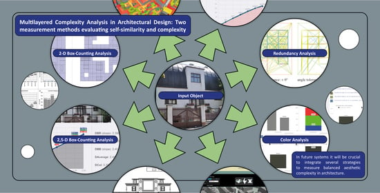
Multilayered Complexity Analysis in Architectural Design: Two Measurement Methods Evaluating Self-Similarity and Complexity

Abstract
:
1. Introduction
1.1. Fractal Geometry and Architecture
1.2. Scalebound and Scaling Shapes
1.3. The Leitmotif
1.4. The Whole and Its Parts
1.5. Complexity and Irregularity
2. Materials and Methods
2.1. Fractal Dimension
- allows the quantitative measurement of mixture between order and surprise in a structure [3]
- gives the visual complexity a quantitative value [3]
- allows to analyze and to compare geometric properties [22]
- enables statements about harmonic relation between the whole and it parts [8]
- enables the comparison of different design solutions [8]
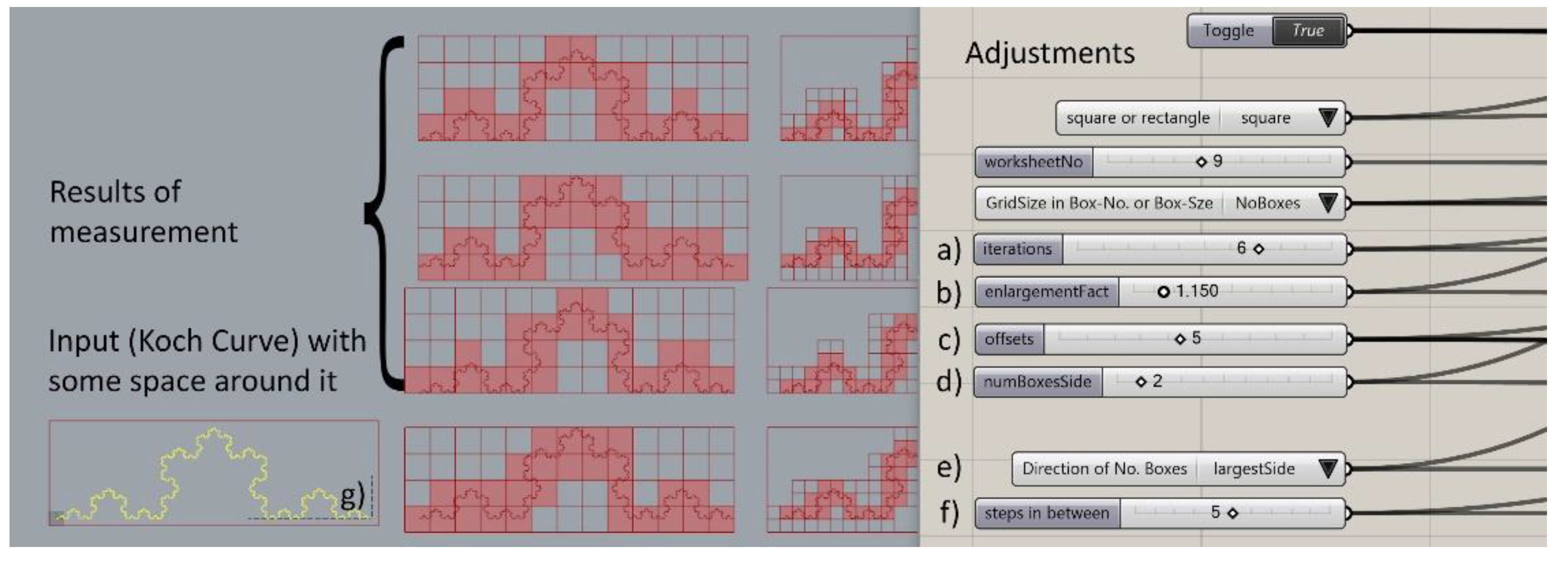
2.2. The Box-Counting Method Applied to 2-Dimensional Line-Graphics
2.2.1. Influence Factors
2.2.2. Implementation
- The box-counting dimension as a result of the minimum number of covering boxes and the corresponding coefficient of determination (which serves as a measure of coherence)
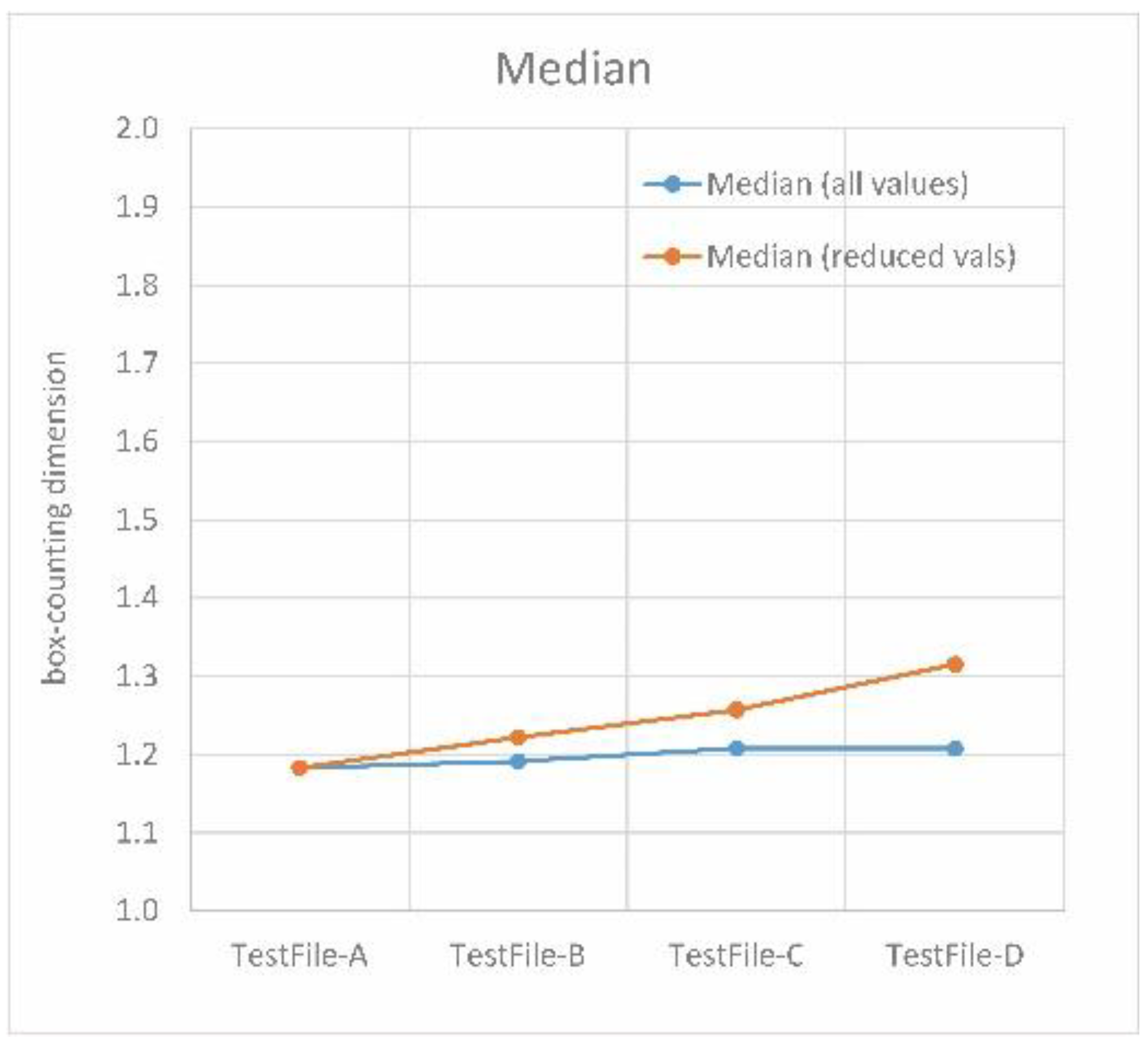
- The median (central value of a data series) of all results visualized in a box-plot, with the interquartile range describing the accuracy of the entire set
- The average of all results
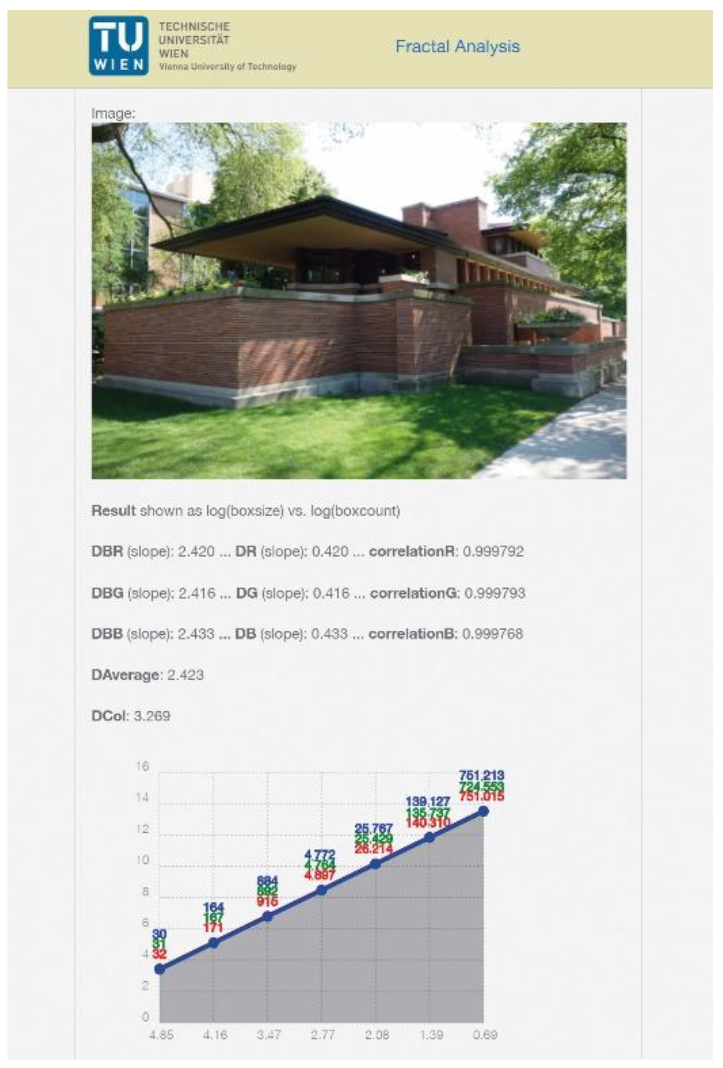
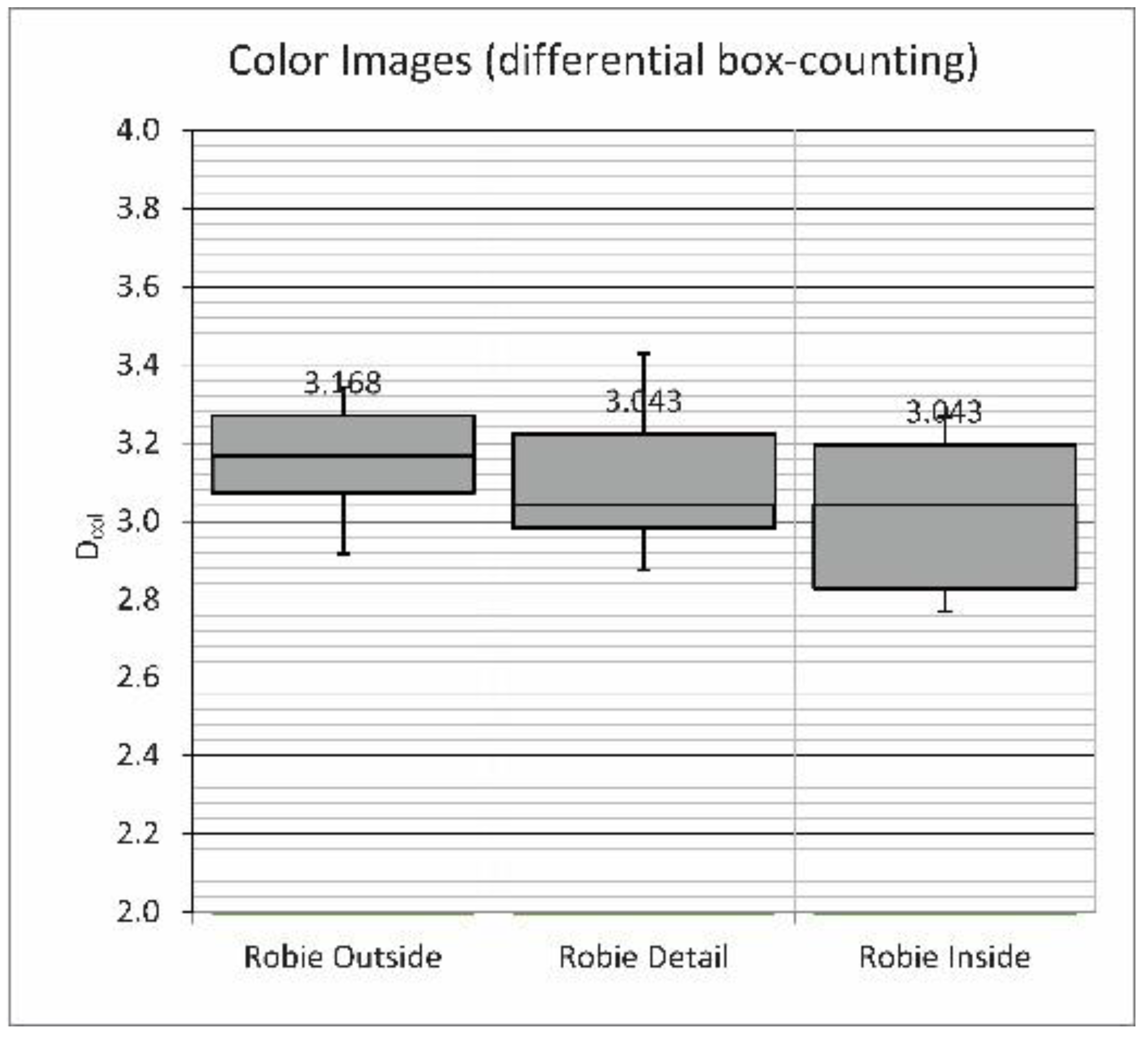
2.3. The Box-Counting Method Applied to Photographs
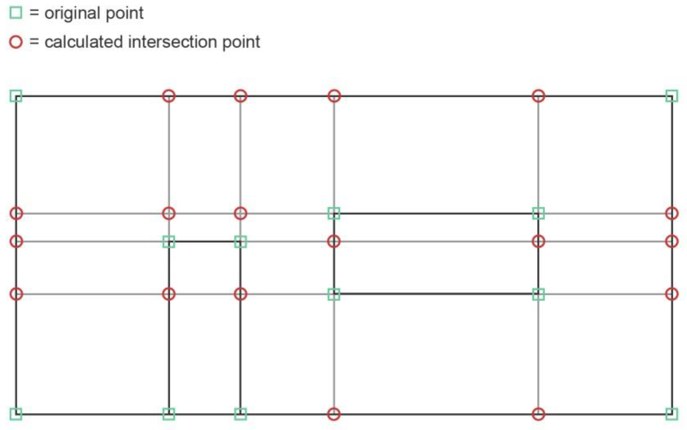
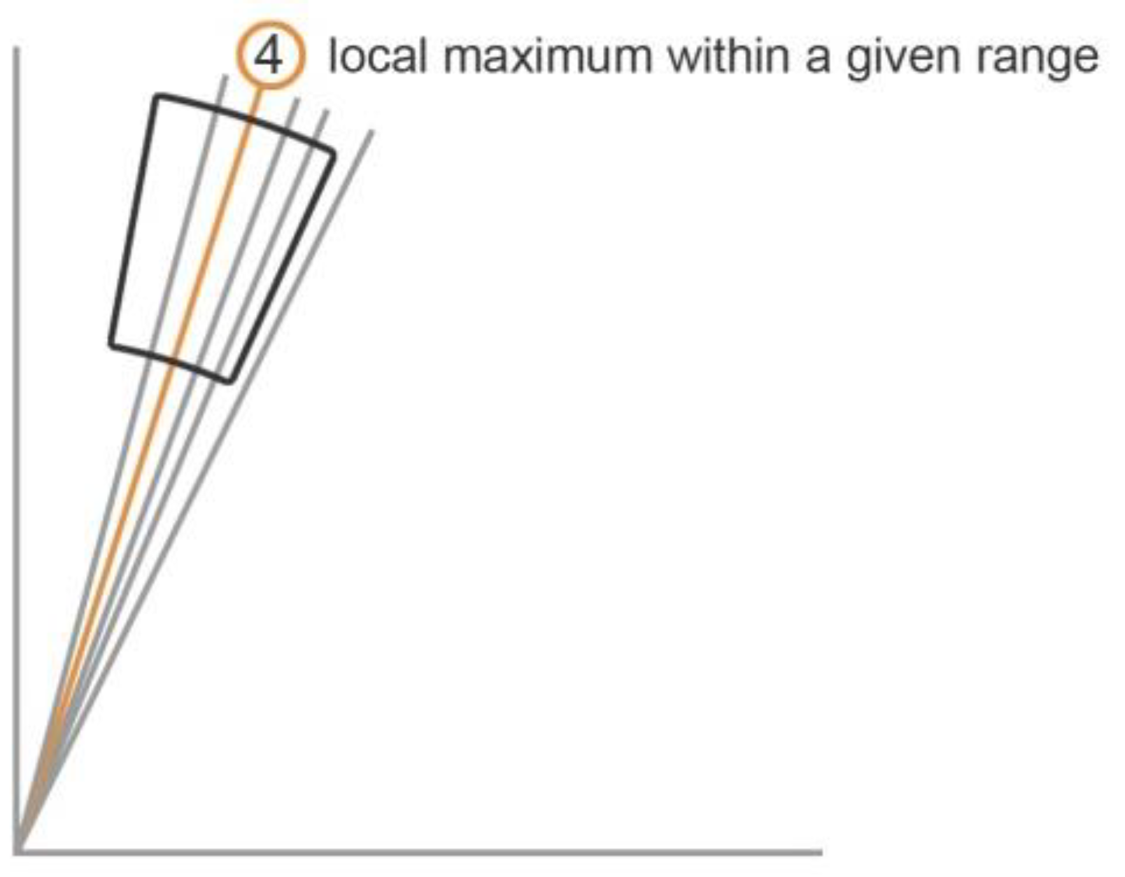
2.4. Redundancy of Proportions, Gradient Analysis and Grid Analysis
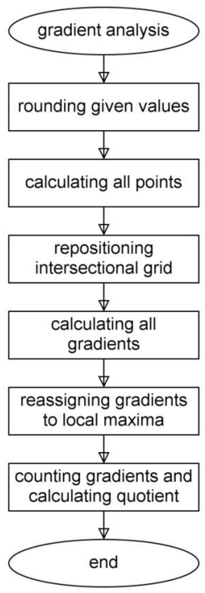
Implementation of the Gradient Analysis
- rounding the values of a given set to represent coordinates on an architecturally relevant scale;
- calculating all points on an orthogonal intersectional grid derived from the given set;
- repositioning of the intersectional grid on the x- and y-axis according to a chosen vertical and horizontal tolerance value (as a percentage of maximum x- and y- distance within the given set);
- calculating all gradients of all possible connections between points;
- calculating local maxima of the gradients according to a chosen tolerance value;
- assigning neighboring values within that chosen range to the gradients representing local maxima;
- listing the remaining gradients and their weight according to the local maxima calculation;
- counting the remaining gradients and forming the quotients of the number of remaining gradients and the possible number of connections based on the original coordinate list as well as the list of all points on the intersectional grid.
3. Results and Discussion
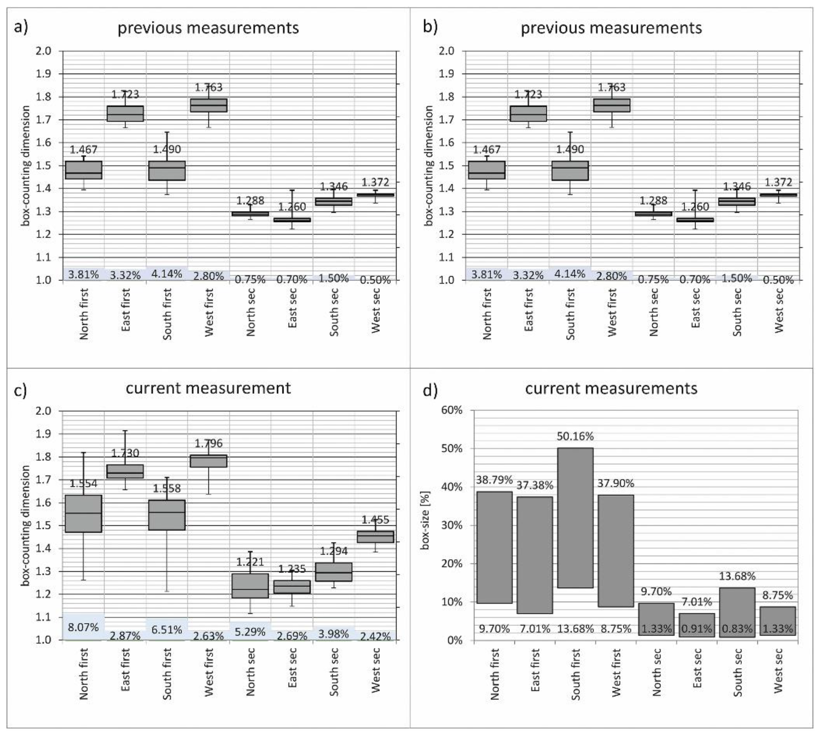
3.1. Box-Counting: Verification of the Data
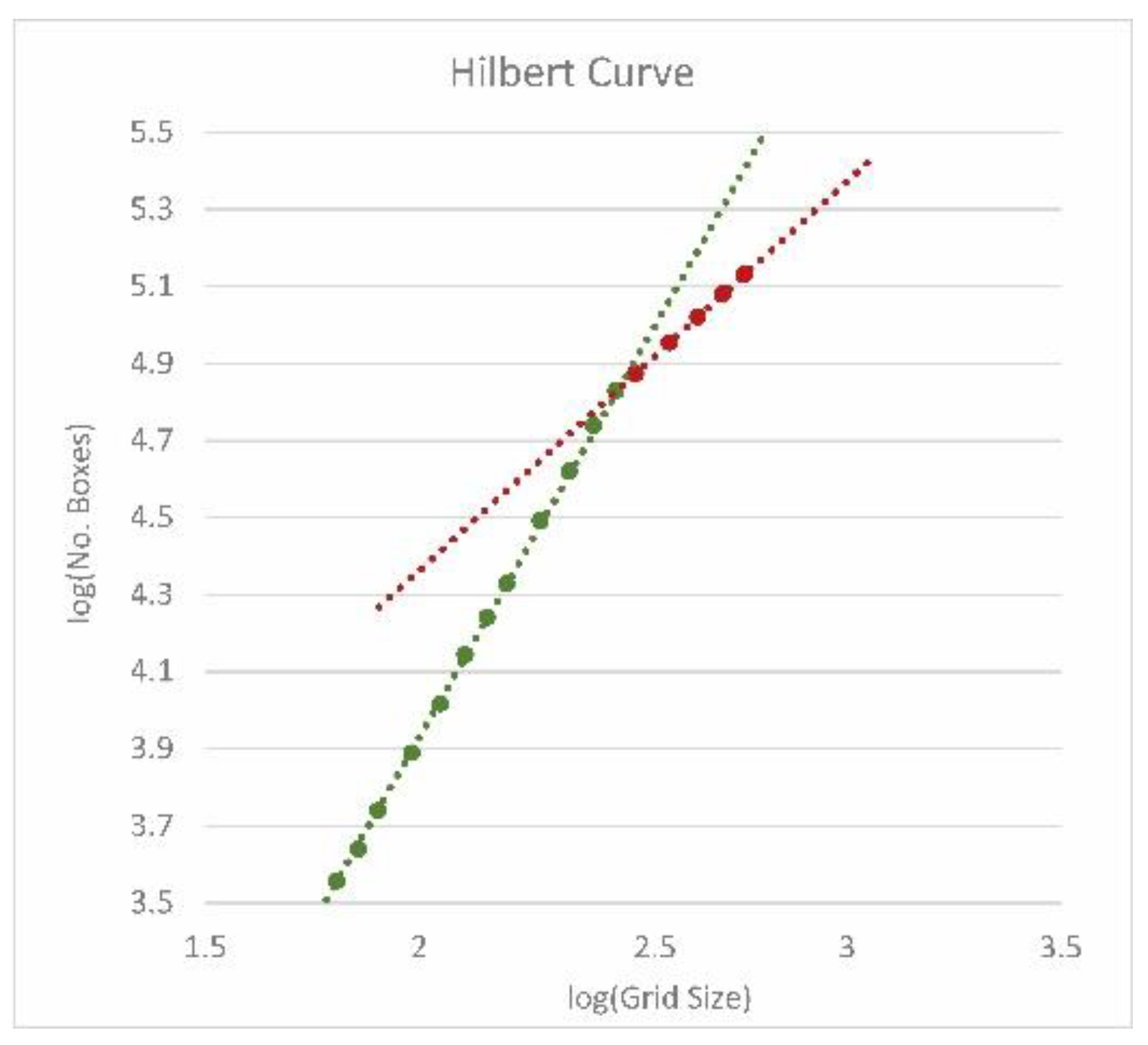
3.2. Box-Counting Applied to Fractal Curves
3.3. Optimized Settings
- Enlargement factor: 1.15
- Number of boxes for the shortest side: 4 (here the authors made a compromise between the two test series of 3 and 5 starting boxes; during the verification phase it turned out that the former worked well for less complex curves, while the latter gave better results for more complex curves)
- Offsets: 5 × 5 (the authors reduced this number due to performance reasons)
- Steps in between: 5 (this value divides the box size in the x-direction between the largest and the next smaller one, whereby the latter is not allowed to be undercut; hence, it defines a maximum value that can change depending on the proportion of the bounding box; e.g., for a square shape and 4 starting boxes for the smallest side, the next smaller grid size equals 8; accordingly, there are only 3 intermediate steps possible; such an adjustment is automatically done by the program)
- Koch curve (= 1.2639, = 1.2619, 0.16%)
- Koch curve with 40° (= 1.0963, = 1.0986, −0.21%)
- Koch curve with 80° (= 1.6041, = 1.6247, −1.27%)
- Minkowski curve (= 1.4782, = 1.50, −1.45%)
- Sierpinski gasket (= 1.5745, = 1.5850, −0.66%)
- Hilbert curve (= 1.9256, = 2.0, −3.72%)
- Peano curve (= 1.9238, = 2.0, −3.81%)
3.4. Box-Counting Applied to Test Cases
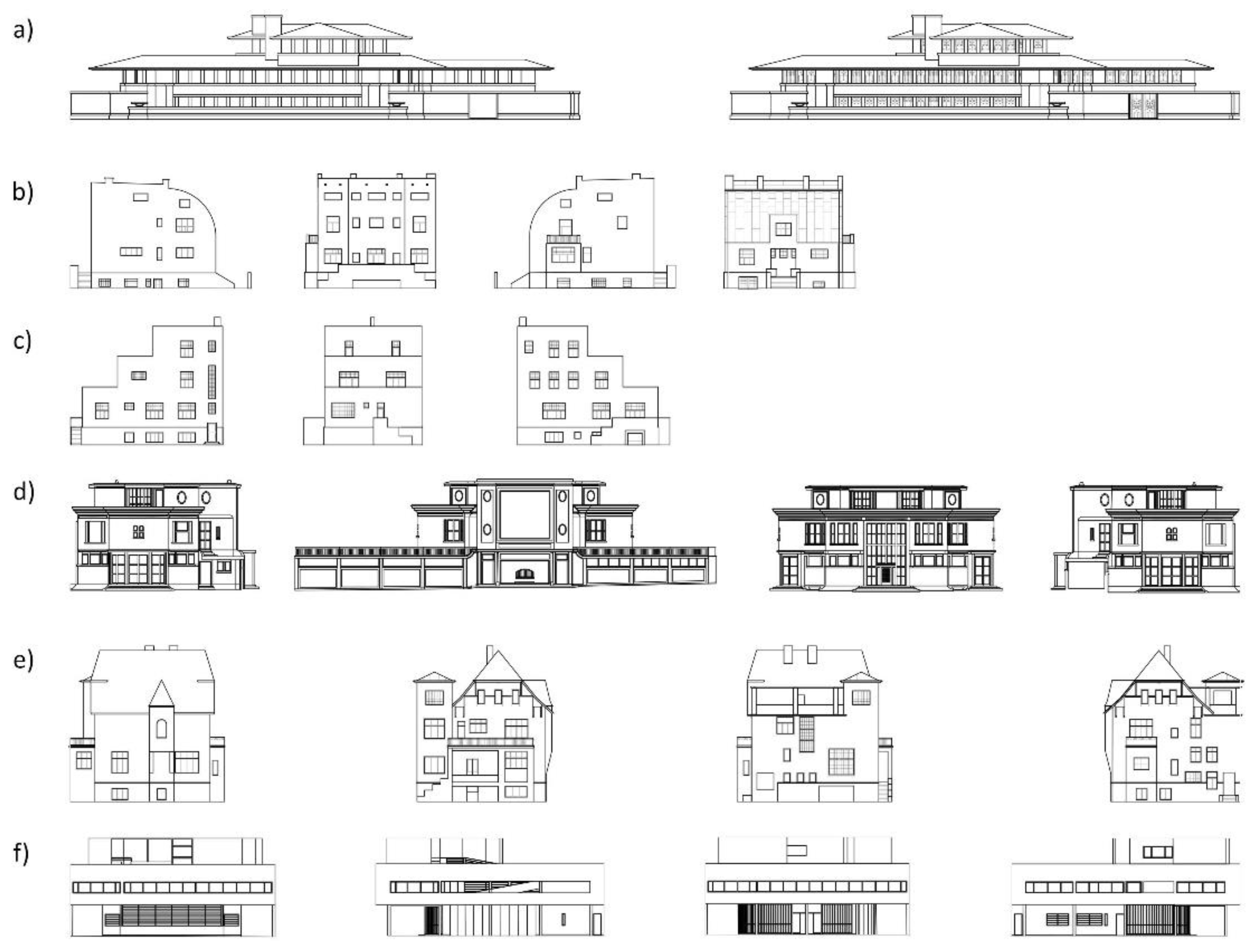
3.5. Box-Counting Applied to Iconic Architecture
3.5.1. Settings
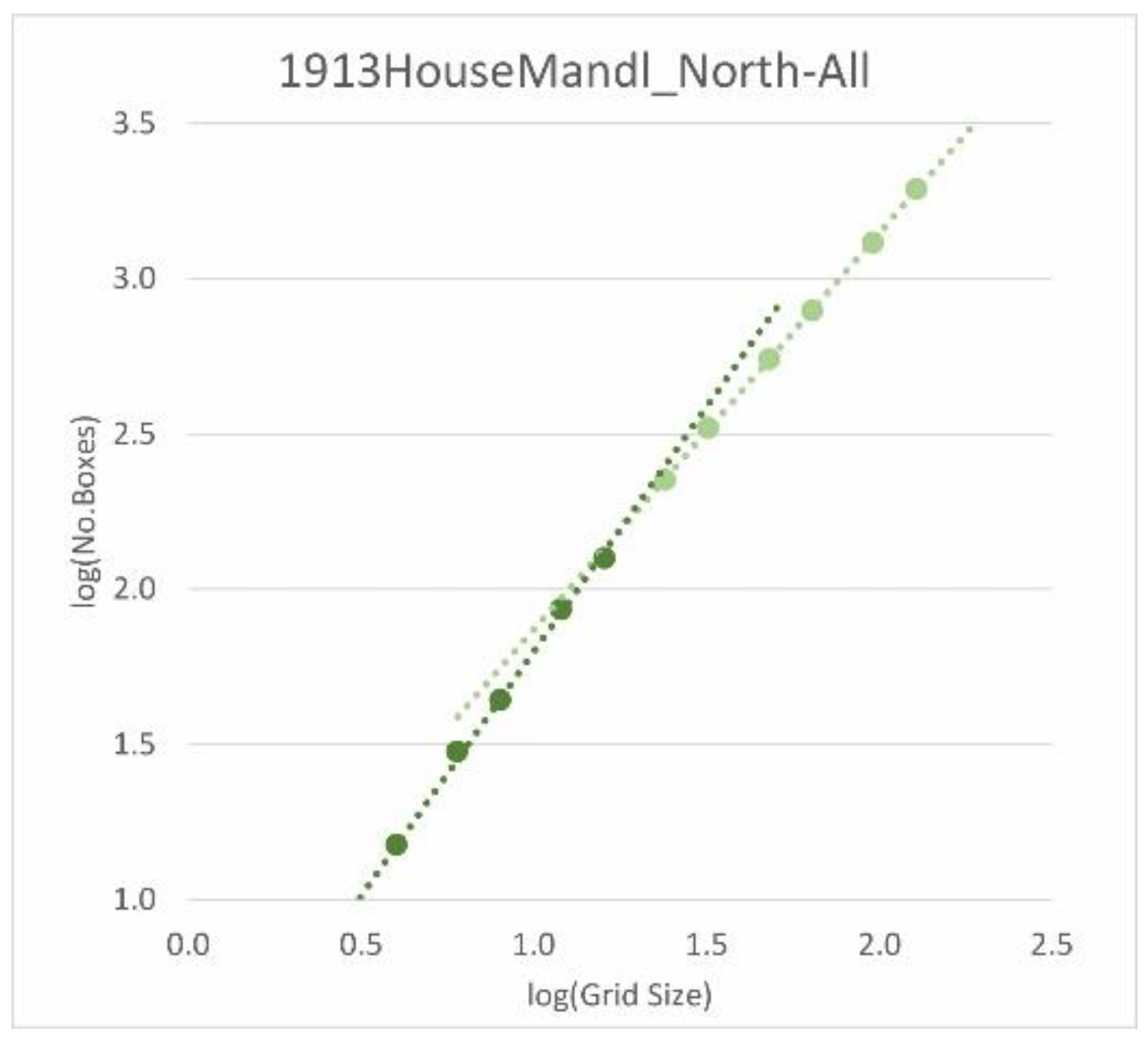
- (1)
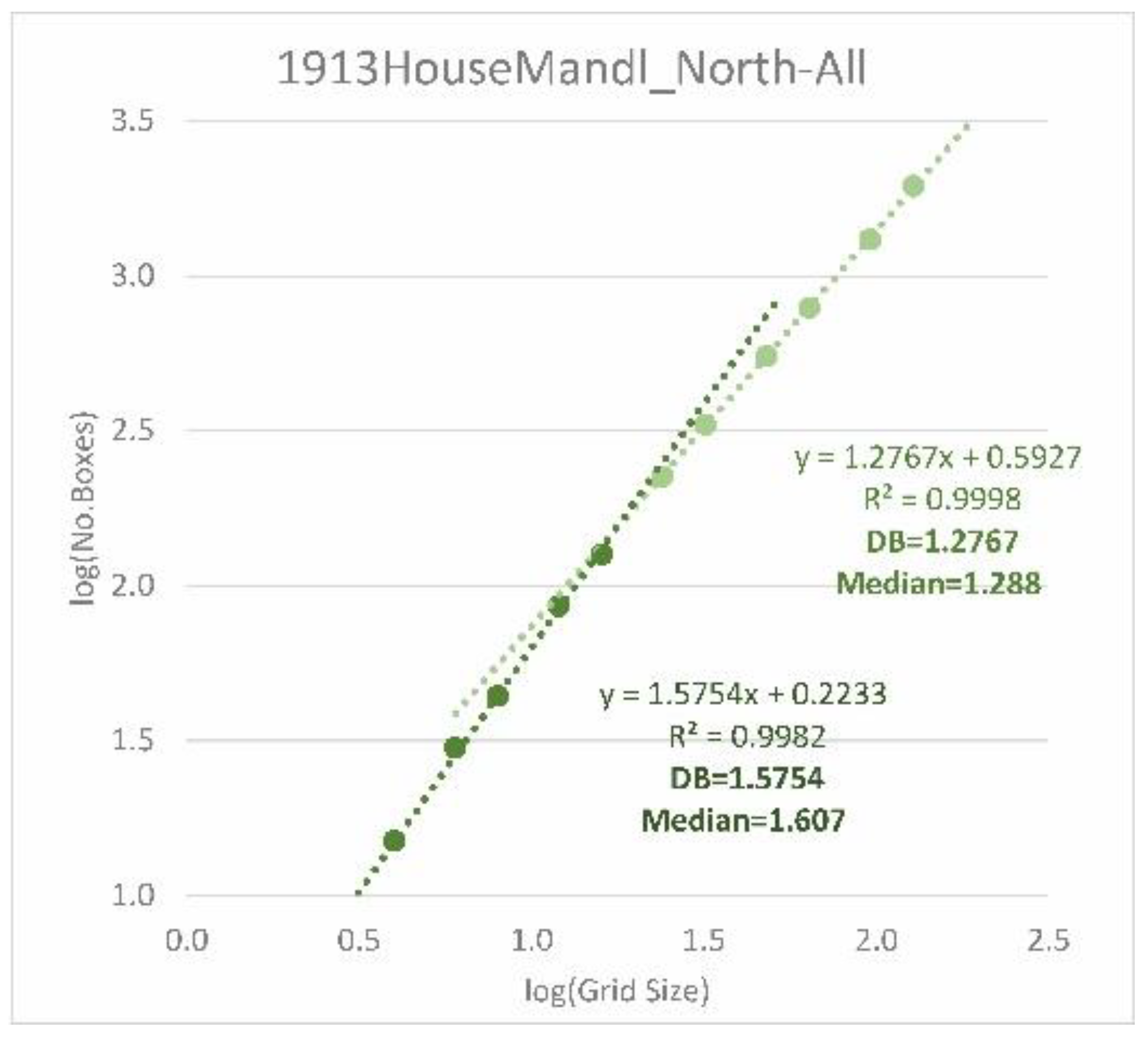
- All data points are very close to the regression line, i.e., there is a clear relationship between box size and number of covered boxes over the entire range under consideration.
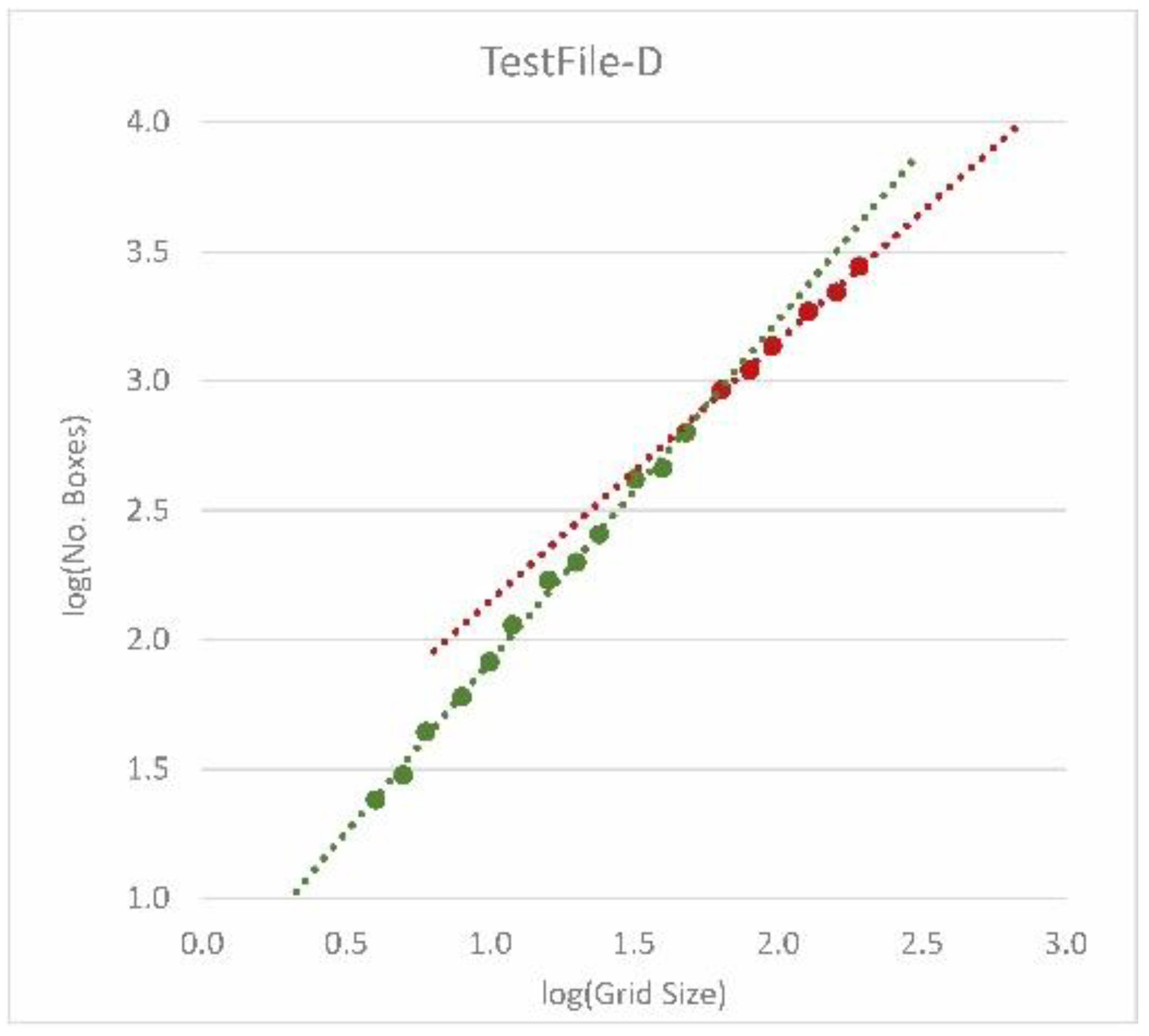
- (2)
- There are two clearly separable intersecting straight segments, with different gradients. Accordingly, a range with larger boxes can lead to higher fractal dimensions, followed by a section with a smaller fractal dimension.
- (3)
- The data points show a continuous curve without straight segments.
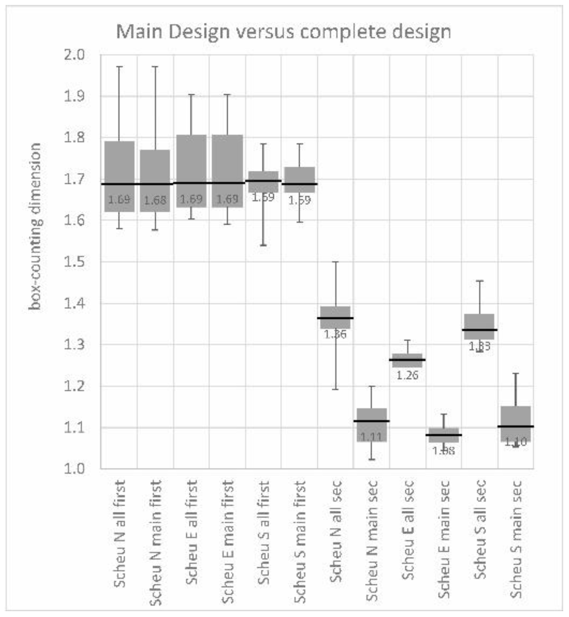
3.5.2. Measurements
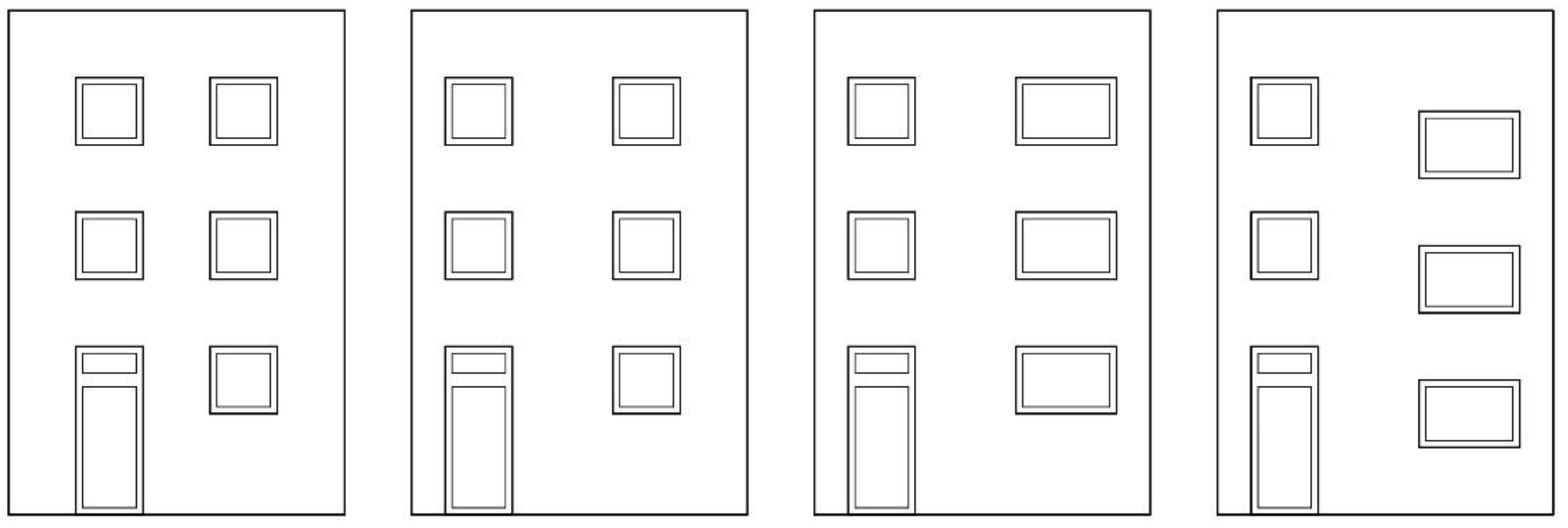
3.6. Gradient Analysis Applied to Test Cases
3.7. Gradient Analysis Applied to Iconic Architecture
4. Conclusions
Author Contributions
Funding
Data Availability Statement
Conflicts of Interest
References
- Mandelbrot, B.B. Die Fraktale Geometrie der Natur; Birkhäuser Verlag: Berlin, Germany, 1991. [Google Scholar]
- Mandelbrot, B.B. Les Objets Fractals: Forme, Hazard et Dimension, 2nd ed.; Flammarion: Paris, France, 1984. [Google Scholar]
- Bovill, C. Fractal Geometry in Architecture and Design; Birkhäuser: Boston, FL, USA, 1996. [Google Scholar]
- Kulcke, M.; Lorenz, W.E. Gradient-Analysis: Method and Software to Compare Different Degrees of Complexity in the Design of Architecture and Design objects. In Real Time, Proceedings of the 33rd International Conference on Education and Research in Computer Aided Architectural Design in Europe, Vol. 1, TU Wien, Vienna, Austria, 16–18 September 2015; Martens, B., Wurzer, G., Grasl, T., Lorenz, W.E., Schaffranek, R., Eds.; Vienna University of Technology: Vienna, Austria, 2015; pp. 415–424. [Google Scholar]
- Lorenz, W.E.; Wurzer, G. FRACAM: A 2.5D Fractal Analysis Method for Facades Test Environment for a Cell Phone Application to Measure Box Counting Dimension. In Anthropologic—Architecture and Fabrication in the Cognitive Age, Proceedings of the 38th International Conference on Education and Research in Computer Aided Architectural Design in Europe, Vol. 1, TU Berlin, Berlin, Germany, 16–18 September 2020; Werner, L.C., Koering, D., Eds.; TU Berlin: Berlin, Germany, 2020; pp. 495–504. [Google Scholar]
- Franck, G.; Franck, D. Architektonische Qualität; Hanser: München, Germany, 2008. [Google Scholar]
- Salingaros, N.A. A Theory of Architecture; Umbau Verlag: Solingen, Germany, 2006. [Google Scholar]
- Lorenz, W.E. Fraktalähnliche Architektur—Einteilung und Messbarkeit: Ein Programm in VBA für AutoCAD. Ph.D. Thesis, TU Wien, Vienna, Austria, 2013. [Google Scholar]
- Mandelbrot, B.B. Scalebound or scaling shapes: A useful distinction in the visual arts and in the natural sciences. Leonardo 1981, 14, 45–47. [Google Scholar] [CrossRef]
- Peitgen, H.-O.; Saupe, D. The Science of Fractal Images; Springer: New York, NY, USA, 1988. [Google Scholar]
- Evers, B. Architekturtheorie: Von der Renaissance bis zur Gegenwart; Taschen Verlag: Köln, Germany, 2006. [Google Scholar]
- Hoffmann, D. Frank Lloyd Wright’s Robie House; Dover Publications, Inc.: Mineola, NY, USA, 1984. [Google Scholar]
- Neumeyer, F. Quellentexte zur Architekturtheorie. Bauen beim Wort Genommen; Prestel: München, Germany, 2002. [Google Scholar]
- Sullivan, L.H. The tall office building artistically considered. Lippincott’s Magazine, 23 March 1896; 403–409. [Google Scholar]
- Kruft, H.-W. Geschichte der Architekturtheorie. Studienausgabe: Von der Antike bis zur Gegenwart; C.H.Beck: München, Germany, 1995. [Google Scholar]
- Le Corbusier. Vers Une Architecture; G. Crès et Cie: Paris, France, 1922. [Google Scholar]
- Lorenz, W.E. Fractals and Fractal Architecture. Master’s Thesis, TU Wien, Vienna, Austria, 2003. [Google Scholar]
- Mandelbrot, B.B. How long is the coast of Britain? Statistical self-similarity and fractional dimension. Science 1967, 156, 636–638. [Google Scholar] [CrossRef] [PubMed] [Green Version]
- Husain, A.; Reddy, J.; Bisht, D.; Sajid, M. Fractal Dimension of Coastline of Australia. Sci. Rep. 2021, 11, 6304. [Google Scholar] [CrossRef] [PubMed]
- Peitgen, H.-O.; Jürgens, H.; Saupe, D. Chaos and Fractals—New Frontiers of Science; Springer: New York, NY, USA, 1992. [Google Scholar]
- Hausdorff, F. Dimension und äußeres Maß. Math. Ann. 1919, 79, 157–179. [Google Scholar] [CrossRef]
- Ostwald, M.J.; Vaughan, J. The Fractal Dimension of Architecture; Birkhäuser: Basel, Switzerland, 2016. [Google Scholar]
- Bovill, C. Fractal Calculations in Vernacular Design. In IASTE Working Paper Series Vol. 97 Critical Methodologies in the Study of Traditional Environments, Proceedings of the International Association for the Study of Traditional Environments (IASTE Conference 14th–17th December 1996, Berkeley); University of California at Berkeley, Centre for Environmental Design: Berkeley, CA, USA, 1997; pp. 35–51. [Google Scholar]
- Vaughan, J.; Ostwald, M.J. Refining the Computational method for the Elevation of Visual Complexity in Architectural Images: Significant Lines in the Early Architecture of Le Corbusier. In The New Realm of Architectural Design, Proceedings of the 27th International Conference on Education and Research in Computer Aided Architectural Design in Europe, Istanbul, Turkey, 6–19 September 2009; Çagdas, G., Colakoglu, B., Eds.; İstanbul Teknik Üniversitesi: Istanbul, Turkey, 2009; pp. 689–696. [Google Scholar]
- Corbit, J.D.; Garbary, D.J. Fractal dimension as a quantitative measure of complexity in plant development. Proc. R. Soc. Lond. Ser. B Biol. Sci. 1995, 262, 1–6. [Google Scholar] [CrossRef]
- Fourtan-Pour, K.; Dutilleul, P.; Smith, D.L. Advances in the implementation of the box-counting method of fractal dimension estimation. Appl. Math. Comput. 1999, 105, 195–210. [Google Scholar] [CrossRef]
- Taylor, R.P. Architect reaches for the clouds. Nature 2001, 410, 18. [Google Scholar] [CrossRef] [PubMed]
- Robert McNeel and Associates. Rhinoceros 3D, Version 6.0; Robert McNeel and Associates: Seattle, WA, USA, 2010. [Google Scholar]
- Wurzer, G.; Lorenz, W.E. FRACAM—Cell Phone Application to Measure Box Counting Dimension. In Protocols, Flows, and Glitches, Proceedings of the 22nd Computer-Aided Architectural Design Research in Asia Conference, Xi’an Jiaotong-Liverpool University, Suzhou, China, 5–8 April 2017; Janssen, P., Loh, P., Raonic, A., Schnabel, M.A., Eds.; Xi’an Jiaotong-Liverpool University: Suzhou, China, 2017; pp. 725–734. [Google Scholar]
- Backes, A.; Bruno, O.M. A New Approach to Estimate Fractal Dimension of Texture Images. In Image and Signal Processing, Proceedings of the 3rd International Conference, ICISP, Cherbourg-Octeville, France, 1–3 July 2008; Elmoataz, A., Lezoray, O., Nouboud, F., Mammass, D., Eds.; Springer: Berlin/Heidelberg, Germany, 2008; pp. 136–143. [Google Scholar] [CrossRef] [Green Version]
- Sarker, N.; Chaudhuri, B.B. An efficient differential box-counting approach to compute fractal dimension of image. IEEE Trans.Syst. Man Cybern. 1994, 24, 115–120. [Google Scholar] [CrossRef] [Green Version]
- Liu, Y.; Chen, L.; Wang, H.; Jiang, L.; Zhang, Y.; Zhao, J.; Wang, D.; Zhao, Y.; Song, Y. An improved differential box-counting method to estimate fractal dimensions of gray-level images. J. Vis. Commun. Image Represent. 2014, 25, 1102–1111. [Google Scholar] [CrossRef]
- Long, M.; Peng, F. A Box-Counting Method with Adaptable Box Height for Measuring the Fractal Feature of Images. Radioengineering 2013, 22, 208–213. [Google Scholar]
- Nayak, S.R.; Mishra, J. On Calculation of Fractal Dimension of Color Images. Int. J. Image Graph. Signal Process. 2017, 9, 33–40. [Google Scholar] [CrossRef] [Green Version]
- GitHub: GetAverageColourAsRGB.js. Available online: Gist.github.com/nucliweb/a3a23febee3ccb9a1b5dc93dadf94fe7 (accessed on 14 April 2020).
- GitHub: Vibrant.js by Zwarts, J. Available online: https://github.com/jariz/vibrant.js/ (accessed on 14 April 2020).
- Color Thief by Dhakar, L. Available online: https://lokeshdhakar.com/projects/color-thief/ (accessed on 14 April 2020). Color Thief is licensed under the MIT License https://github.com/lokesh/color-thief/blob/master/LICENSE.
- Rowland, I.D.; Howe, T.N. Vitruvius—Ten Books on Architecture; Cambridge University Press: Cambridge, UK, 1999. [Google Scholar]
- Kulcke, M.; Lorenz, W.E. Utilizing Gradient Analysis within Interactive Genetic Algorithms. In Complexity & Simplicity, Proceedings of the 34th International Conference on Education and Research in Computer Aided Architectural Design in Europe, Vol. 2, University of Oulu, Oulu, Finland, 22–26 August 2016; Herneoja, A., Österlund, T., Markkanen, P., Eds.; University of Oulu: Oulu, Finland, 2016; pp. 359–364. [Google Scholar]
- Cube, F. Kybernetische Grundlagen des Lernens und Lehrens; Ernst Klett Verlag: Stuttgart, Germany, 1965. [Google Scholar]
- Kulcke, M. Gestaltkonfiguration und Verantwortung. Ph.D. Thesis, HafenCity University, Hamburg, Germany, 2019. [Google Scholar]
- Guski, R. Wahrnehmen—Ein Lehrbuch; Kohlhammer: Stuttgart, Germany, 1996. [Google Scholar]
- Koch, H. Sur une courbe continue sans tangente, obtenue par une construction géométrique élémentaire. Ark. Mat. Astron. Fys. 1904, 1, 681–702. [Google Scholar]
- Maertens, H. Der Optische Maßstab: Oder die Theorie und Praxis des Asthetischen Sehens in der Bildenden Kunst; Wasmuth: Berlin, Germany, 1884. [Google Scholar]
- Ostwald, M.J.; Vaughan, J.; Tucker, C. Characteristic Visual Complexity: Fractal Dimensions in the Architecture of Frank Lloyd Wright and Le Corbusier. Nexus Archit. Math. 2008, 7, 217–232. [Google Scholar] [CrossRef]
- Lorenz, W.E. Measurability of Loos’ rejection of the ornament: Using box-counting as a method for analyzing facades. In Fusion, Proceedings of the 32nd International Conference on Education and Research in Computer Aided Architectural Design in Europe, Vol. 1, Northumbria University, Newcastle upon Tyne, UK, 10–12 September 2014; Thompson, E.M., Ed.; Northumbria University: Newcastle upon Tyne, UK, 2014; pp. 495–504. [Google Scholar] [CrossRef]


| House Steiner: North Elevation | Angles: | 18° | 27° | 45° |
|---|---|---|---|---|
| Approximate distances: | 40.50 m | 25.80 m | 13.20 m | |
| Distance corresponds to: | Overview | Overview with environment | Single parts | |
| 0°10′ | 11.80 cm | 7.50 cm | 3.85 cm | |
| 1°00′ | 0.85 m | 0.50 m | 0.25 m | |
| 7°26′ | 6.35 m | 3.60 m | 1.75 m | |
| 10°00′ | 8.55 m | 4.85 m | 2.35 m |
Publisher’s Note: MDPI stays neutral with regard to jurisdictional claims in published maps and institutional affiliations. |
© 2021 by the authors. Licensee MDPI, Basel, Switzerland. This article is an open access article distributed under the terms and conditions of the Creative Commons Attribution (CC BY) license (https://creativecommons.org/licenses/by/4.0/).
Share and Cite
Lorenz, W.E.; Kulcke, M. Multilayered Complexity Analysis in Architectural Design: Two Measurement Methods Evaluating Self-Similarity and Complexity. Fractal Fract. 2021, 5, 244. https://doi.org/10.3390/fractalfract5040244
Lorenz WE, Kulcke M. Multilayered Complexity Analysis in Architectural Design: Two Measurement Methods Evaluating Self-Similarity and Complexity. Fractal and Fractional. 2021; 5(4):244. https://doi.org/10.3390/fractalfract5040244
Chicago/Turabian StyleLorenz, Wolfgang E., and Matthias Kulcke. 2021. "Multilayered Complexity Analysis in Architectural Design: Two Measurement Methods Evaluating Self-Similarity and Complexity" Fractal and Fractional 5, no. 4: 244. https://doi.org/10.3390/fractalfract5040244
APA StyleLorenz, W. E., & Kulcke, M. (2021). Multilayered Complexity Analysis in Architectural Design: Two Measurement Methods Evaluating Self-Similarity and Complexity. Fractal and Fractional, 5(4), 244. https://doi.org/10.3390/fractalfract5040244