Article

Stability Analysis and Numerical Computation of the Fractional Predator–Prey Model with the Harvesting Rate

1
Department of Mathematics and Computer Sciences, Necmettin Erbakan University, 42090 Konya, Turkey
2
Department of Mathematics, College of Engineering, Mathematics and Physical Sciences, University of Exeter, Penryn Campus, Cornwall TR10, UK
3
Laboratoire Lmdan, Département de Mathématiques de la Décision, Université Cheikh Anta Diop de Dakar, Faculté des Sciences Economiques et Gestion, Dakar Fann BP 5683, Senegal
*
Authors to whom correspondence should be addressed.
Fractal Fract. 2020, 4(3), 35; https://doi.org/10.3390/fractalfract4030035
Submission received: 23 May 2020 / Revised: 13 July 2020 / Accepted: 14 July 2020 / Published: 16 July 2020

Abstract

:
In this work, a fractional predator-prey model with the harvesting rate is considered. Besides the existence and uniqueness of the solution to the model, local stability and global stability are experienced. A novel discretization depending on the numerical discretization of the Riemann–Liouville integral was introduced and the corresponding numerical discretization of the predator–prey fractional model was obtained. The net reproduction number R 0 was obtained for the prediction and persistence of the disease. The dynamical behavior of the equilibria was examined by using the stability criteria. Furthermore, numerical simulations of the model were performed and their graphical representations are shown to support the numerical discretizations, to visualize the effectiveness of our theoretical results and to monitor the effect of arbitrary order derivative. In our investigations, the fractional operator is understood in the Caputo sense.

1. Introduction

Fractional calculus (FC) is a common field trying to understand the real-world phenomena that are modeled with non-integer-order derivatives and it is a field wherein the differentiation and the integrations are done with non-integer order derivatives as well. A fractional derivative, one can understand, is a type of derivative in which the order is non-integer-based but satisfies certain conditions: when the order of the derivative is zero we have the primary function, and when the order is one we converge to the first order integer order derivative [1]. The advantages of the fractional derivatives are the memory impact and the illustrative physical properties that are conserved. Using these types of operators, more effective and up-to-date studies have been revealing over time. In this context, fractional calculus theory and its illustrative applications are attracting attention all over the world day by day. New fractional operators that have different features have been defined and have been used extensively to model real-life problems. The emergence of the new operators in the literature can be considered as a result of the reproduction of new problems that model different types of real-life events. Fractional derivative operators that address the kind of nonlinear differential equations can be stated as non-local. There exist nowadays, many types of fractional derivatives with and without singular kernels. The fractional derivative begins with Leibniz’s question in 1695. The list of the existing fractional derivatives is very long. With singular kernels, we have the Caputo–derivative [2], the Riemann–Liouville derivative [2] and the Katugampola derivative [3]. Without singular kernels, we have two types: the fractional derivative with an exponential kernel known as the Caputo–Fabrizio fractional derivative (CF) [4] and the fractional derivative with a Mittag–Leffler kernel known as the Atangana–Baleanu fractional derivative (ABC) [5]. Due to the memory effect, the non-integer models integrate all previous information from the past that makes it easier for them to predict and translate the epidemic models more accurately. Because of effective properties, fractional order calculus has found wide applications to model dynamics processes in many well-known fields, such as biology [6,7,8,9,10,11], physics [12,13,14,15,16], finance and economics [17,18], science and engineering [19,20], mechanics and mathematical modeling [21,22]. We enumerate numerous fractional operators in the literature [23,24,25,26,27]. Moreover, some numerical and approximate solution methods and their illustrative applications have been stated in [28,29,30,31,32,33,34,35,36,37,38,39,40,41,42,43,44,45,46,47,48,49,50].
Regarding modeling the predator–prey model (P–PM) with a fractional-order derivative, the numerical discretizations and the simulations are the subjects of research in this present paper. The P–PM has been considered in the context of the Caputo fractional derivative [1,51,52]. There exist many investigations related to the predator–prey models. In [53], Li et al. have proposed the stability analysis of the P–PM with harvesting. They have also provided graphical representations to support their results. In [54], the authors presented the predator–prey model under a reserved area. The authors have provided a new predator–prey model, proposed the equilibrium points, and investigated their stability analysis. In [55], Seo et al. have presented the P–PM with a Holling type functional response. In [56], Suryando et al. have proposed investigations related to the fractional P–PM with the functional response and harvesting. The authors have proposed as well the stability analysis of the equilibrium points of their proposed model. In [57], Tang presented a scientific report on predator–prey dynamics. In [58], Elettreby et al. have presented the stability analysis and the numerical simulations of the P–PM with a fractional order derivative and with a two prey, one predator system. In [59], Liu et al. have proposed the numerical solutions of a fractional P–PM and many others [60,61,62,63,64,65,66,67].
In this paper, we consider the predator–prey model with the Caputo fractional derivative and with the harvesting rate. The main objective of this paper is to propose a new numerical scheme base on the numerical scheme of the Riemann–Liouville integral to construct numerical discretizations of the fractional predator–prey model with the harvesting rate. The graphics of the solutions of the fractional equations will be proposed to support the numerical discretizations. We are mainly motivated by the fact in the literature, many investigations related to the predator–prey models investigate stability analysis. Here, after stability analysis, we propose a new numerical scheme. This issue will permit us to analyze the impact of the harvesting rate on the processes carefully.
The paper is divided as follows: In Section 2, we recall the fractional tools for our investigations. We deal with the Caputo derivative and Riemann–Liouville integral in our investigations throughout the paper. We also recall some properties related to the fractional derivatives. In Section 3, we present the predator–prey model in the context of the Caputo derivative. We focus on the qualitative properties of the solution in Section 4. In Section 5, we investigate the both local and global stability analyses of the equilibrium points of the predator–prey model. In Section 6, the novel numerical discretization of the fractional P–PM is proposed. In Section 7, we support the numerical discretizations by graphical representations. Final remarks are assigned in Section 8.

2. Some Preliminaries

In this section, we give the fundamental definitions that can be used throughout the paper. These definitions generally explain the fractional derivative in the power kernel sense.
Definition 1
([1]). The Riemann–Liouville (R–L) representation of fractional integral operator of order γ > 0 of a function φ : ( 0 , ) R is given by
0 R L D t γ φ ( t ) = 0 R L I t γ φ ( t ) = 1 Γ ( γ ) 0 t ( t τ ) γ 1 φ ( τ ) d τ , t > 0 ,
0 R L I t 0 ψ ( τ ) = ψ ( τ ) ,
where γ > 0 and Γ . is the Gamma function.
Definition 2
([1]). The R–L representation of fractional operator of order γ > 0 of a function φ : ( 0 , ) R is given by
0 R L D t γ φ ( t ) = 1 Γ ( n γ ) d d t n 0 t φ ( τ ) ( t τ ) γ n + 1 d τ , 0 n 1 < γ < n , n = [ γ ] , d d t n φ ( t ) , γ = n N .
Definition 3
([1]). The Caputo fractional operator of order γ > 0 of a function φ : ( 0 , ) R is given by
0 C D t γ φ ( t ) = 1 Γ ( n γ ) 0 t d / d τ n φ ( τ ) ( t τ ) γ n + 1 d τ , 0 n 1 < γ < n , n = [ γ ] , n N , d d t n φ ( t ) , γ = n , n N .
where the operator 0 C D t γ satisfies:
0 C D t γ 0 R L I t γ φ ( t ) = φ ( t ) and 0 R L I t γ 0 C D t γ φ ( t ) = φ ( t ) v = 0 n 1 φ ( v ) ( u ) v ! ( t u ) v , t > u .
Definition 4
([1]). The Laplace of the Caputo fractional operator of a function φ ( t ) of order γ > 0 is presented with
L 0 C D t γ φ t = s γ φ ( s ) v = 0 n 1 φ v ( 0 ) s γ v 1 .
We introduce two lemmas which will be used to establish local stability and global stability, respectively. The first lemma is called the Matignon criterion and the second one is the Lyapunov characterization for global stability.
Lemma 1
([68]). The fractional differential equation 0 C D t γ x = P x , with P R n × n , x ( t 0 ) = x 0 , 0 < γ < 1 and x R n , is local asymptotically stable if only if
arg s p c P > γ π 2 ,
where s p c ( P ) is considered as the spectrum of the matrix P .
Lemma 2
([69]). We assume the vectors w R n which are differentiables. Under the assumption t t 0 , we have the following condition
0 C D t γ w w * w * ln w w * 1 w w * 0 C D t γ w , w i t h   w * R + n .

3. Fractional Predator–Prey Model with Caputo Derivative

In this paper, we present the predator–prey model in the context of the fractional operator. Note that the fractional-order derivatives are more accurate at modeling biological processes since these types of operators consider the memory impact which gives more realistic results in real-life models. It is the deterministic property of the dynamical system. The following dynamics represent the fractional equation proposed in this section [53,70,71]
0 C D t γ x = r x 1 x k a x y ,
0 C D t γ y = a c x y d y H y ,
where 0 C D t γ represents the Caputo fractional derivative which is given in Definition 3. We consider the initial conditions defined by
x ( 0 ) = x 0 , y ( 0 ) = y 0 ,
where x denotes the prey species; y represents the predator species; the prey increases logistically with the growth rate denoted by r and the carrying capacity k; a represents the rate of predation; c denotes the efficiency of predation; d is the mortality rate of the predator species; and H y represents the harvesting function.
Now, we consider the model of Equations (7) and (8). Firstly, we describe harvesting function H y of the predators in our model, Equations (7) and (8), which has the following form
H y = m y , 0 y y 0 , h , y 0 < y .
Using the model in Equations (7) and (8) as our baseline model, we suppose that harvesting takes place, but only the predator population is under harvesting, and introduce harvesting function H y of the predator to prey-predator model in Equations (7) and (8) for discussing its dynamical features. We assume that the harvesting rate is proportional to the predator population size until it reaches a threshold value due to limited facilities of harvesting or resource protection. Let us show the harvesting threshold value as h = m y 0 ; thus Equations (7) and (8) can be written as the following equations for 0 y y 0
0 C D t γ x = r x 1 x k a x y , 0 C D t γ y = a c x y d y m y .
When y 0 < y , then the system in Equations (7) and (8) turns to the following
0 C D t γ x = r x 1 x k a x y , 0 C D t γ y = a c x y d y h .

Positivity and Boundedness

In this subsection, the positivity and boundedness of the solution for the proposed model (Equations (7) and (8)) are given. Let R + 2 = χ ( t ) R 2 : χ ( t ) 0 and χ ( t ) = x t , y t T .
Theorem 1.
The solution of the proposed fractional-order model (Equations (7) and (8)) along initial conditions (9) is bounded in R + 2 . Moreover, the density of the population remains in a nonnegative region.
Proof. 
Let the function W ( t ) = x + 1 c y and λ be a positive constant. Applying the Caputo derivative, we have the following relationship
0 C D t γ W + λ W = r x 2 k + r x d y c H y c + λ x + λ c y = r x 2 k + r + λ x + λ c d c y H y c = r k x 2 k ( r + λ ) r x + λ c d c y H y c r k x k ( r + λ ) 2 r 2 + k ( r + λ ) 2 4 r ,
where λ < d + m . From the property in [72] and using comparison principle, since t converges to infinity, we have the following relationship
W ( t ) W ( 0 ) E γ λ t γ + k ( r + λ ) 2 4 r t γ E γ , γ + 1 λ t γ k ( r + λ ) 2 4 r ,
where E γ , β . is the Mittag–Leffer function of two parameters. Finally, the following set in the domain R + 2 is positively invariant
A = x ( t ) , y ( t ) R + 2 | x ( t ) 0 , y ( t ) 0 , x + 1 c y k ( r + λ ) 2 4 r .
 □
We have replaced the classical derivative by the Caputo derivative in the study. It is important to justify the replacement and to prove the physical meanings of the new model. Another point is also to show that the solution to the new model exists and is unique. All these points will be discussed in the next sections.

4. Qualitative Properties of the P–PM

In this Part, we give the qualitative properties of the solutions of the predator–prey model which is given in the system (7) and (8). Firstly we start by taking the Riemann–Liouville integral which is given in Definition 1 of both sides the mentioned system and we get
x t x 0 = 0 R L I t γ r x 1 x k a x y , y t y 0 = 0 R L I t γ a c x y d y H y ,
which gives the following Volterra-type integral equations:
x t x 0 = 1 Γ γ 0 t t τ γ 1 r x τ 1 x τ k a x τ y τ d τ , y t y 0 = 1 Γ γ 0 t t τ γ 1 a c x τ y τ d y τ H y d τ .
Let us define the following kernels as
φ t , x , y = r x t 1 x t k a x t y t , ϕ t , x , y = a c x t y t d y t H y .
Then the following theorem arises:
Theorem 2.
The kernels φ and ϕ satisfy the Lipschitz assumptions and contractions if the following inequality is verified:
0 z 1 , z 2 < 1 .
where x q , y l , z 1 = r + a l + 2 q r / k , q , l 0 and z 2 = a c q + d , or z 2 = a c q + d + m , for the constant harvesting rate or depending on the predator population, respectively.
Proof. 
Let x 1 and x 2 be two functions for the kernel φ ; and y 1 and y 2 be two functions for the kernel ϕ . Then we have
φ t , x 1 , y φ t , x 2 , y = r x 1 1 x 1 k a x 1 y r x 2 1 x 2 k + a x 2 y , r + a l + 2 q r k x 1 x 2 , z 1 x 1 x 2 ,
and
φ t , x , y 1 φ t , x , y 2 = a c x y 1 d y 1 h a c x y 2 + d y 2 + h , a c q + d y 1 y 2 , z 2 y 1 y 2 ,
or
φ t , x , y 1 φ t , x , y 2 = a c x y 1 d y 1 m y 1 a c x y 2 + d y 2 + m y 2 , a c q + d + m y 1 y 2 , z 2 y 1 y 2 ,
where . is the Euclidean norm, x q , y l , z 1 = r + a l + 2 q r / k and z 2 = a c q + d , or z 2 = a c q + d + m , for the constant harvesting rate or depending on the predator population, respectively. Therefore, the Lipschitz conditions are satisfied for kernels φ and ϕ , and if 0 z 1 , z 2 < 1 , then z 1 and z 2 are also contractions for φ and ϕ , respectively. This proofs the theorem. □
By considering the kernels φ and ϕ , we can rewrite the system which is given in Equation (16) as follows:
x t = x 0 + 1 Γ γ 0 t t τ γ 1 φ τ , x , y d τ , y t = y 0 + 1 Γ γ 0 t t τ γ 1 ϕ τ , x , y d τ .
We can proceed with the following recursive formula
x n t = x 0 + 1 Γ γ 0 t t τ γ 1 φ τ , x n 1 , y d τ , y n t = y 0 + 1 Γ γ 0 t t τ γ 1 ϕ τ , x , y n 1 d τ ,
where x 0 t = x 0 and y 0 t = y 0 . Then we can write
Ψ n t = x n t x n 1 t = 1 Γ γ 0 t t τ γ 1 φ τ , x n 1 , y φ τ , x n 2 , y d τ , Φ n t = y n t y n 1 t = 1 Γ γ 0 t t τ γ 1 ϕ τ , x , y n 1 ϕ τ , x , y n 2 d τ ,
where x n t = j = 1 n Ψ n t and y n t = j = 1 n Φ n t . By taking the norm of both sides of Equation (24), we have
Ψ n t = x n t x n 1 t 1 Γ γ 0 t t τ γ 1 φ τ , x n 1 , y φ τ , x n 2 , y d τ , Φ n t = y n t y n 1 t 1 Γ γ 0 t t τ γ 1 ϕ τ , x , y n 1 ϕ τ , x , y n 2 d τ .
Since the kernels satisfy the Lipschitz condition (see Theorem 2), we get
x n t x n 1 t z 1 Γ γ 0 t t τ γ 1 x n 1 x n 2 d τ , y n t y n 1 t z 2 Γ γ 0 t t τ γ 1 y n 1 y n 2 d τ .
Then we achieve from the last inequality
Ψ n t z 1 Γ γ 0 t t τ γ 1 Ψ n 1 τ d τ , Φ n t z 2 Γ γ 0 t t τ γ 1 Φ n 1 τ d τ .
These results give us the following theorem:
Theorem 3.
The predator–prey model defined by the fractional operator with the power kernel has a solution under the condition that we are able to find t m a x holding:
z i t m a x γ Γ γ + 1 < 1 , i = 1 , 2 .
Proof. 
Considering the functions x t and y t are bounded and their kernels φ and ϕ hold the Lipschitz condition, we can give the following by taking Equation (27) into account,
Ψ n t x 0 t z 1 t m a x γ Γ γ + 1 n , Φ n t y 0 t z 2 t m a x γ Γ γ + 1 n .
Now we show that the functions in Equation (29) are the solutions of the given predator–prey model. We suppose
x t x 0 = x n t p n t , y t y 0 = y n t q n t ,
where p n and q n are remaining terms. Then we will demonstrate that the terms which are given in Equation (30) hold that p t 0 and q t 0 . Since we have
p n t 1 Γ γ 0 t t τ γ 1 φ τ , x , y φ τ , x n 1 , y d τ 1 Γ γ 0 t t τ γ 1 φ τ , x , y φ τ , x n 1 , y d τ t γ z 1 Γ γ + 1 x x n 1 ,
and
q n t 1 Γ γ 0 t t τ γ 1 ϕ τ , x , y ϕ τ , x , y n 1 d τ 1 Γ γ 0 t t τ γ 1 ϕ τ , x , y ϕ τ , x , y n 1 d τ t γ z 2 Γ γ + 1 y y n 1 ,
repeating this process recursively, we get
p n t t γ Γ γ + 1 n + 1 z 1 n N ,
and
q n t t γ Γ γ + 1 n + 1 z 2 n N .
Considering these last two inequalities at t m a x point, we have
p n t t m a x γ Γ γ + 1 n + 1 z 1 n N ,
and
q n t t m a x γ Γ γ + 1 n + 1 z 2 n N .
For the last step, after applying the limit to both sides of the last inequalities as n , and by taking into account the results of Theorem 2, we get p t 0 and q t 0 .  □
Theorem 4.
The predator–prey model defined by the fractional operator with the power kernel in Equations (7) and (8) has a unique solution.
Proof. 
Let say there exists another solution of the system, namely, x 1 t and y 1 t . Then we can write
x t x 1 t = 1 Γ γ 0 t t τ γ 1 φ τ , x , y φ τ , x 1 , y d τ , y t y 1 t = 1 Γ γ 0 t t τ γ 1 ϕ τ , x , y ϕ τ , x , y 1 d τ .
If we apply the norm to both sides of Equation (33), we obtain
x t x 1 t 1 Γ γ 0 t t τ γ 1 φ τ , x , y φ τ , x 1 , y d τ , y t y 1 t 1 Γ γ 0 t t τ γ 1 ϕ τ , x , y ϕ τ , x , y 1 d τ .
Since the Lipschitz condition is satisfied by the kernels φ and ϕ , we can write
x t x 1 t z 1 t γ Γ γ + 1 x t x 1 t , y t y 1 t z 2 t γ Γ γ + 1 y t y 1 t ,
which gives
x t x 1 t 1 z 1 t γ Γ γ + 1 0 , y t y 1 t 1 z 2 t γ Γ γ + 1 0 .
Hence, we have x t x 1 t = 0 and y t y 1 t = 0 which gives x t = x 1 t and y t = y 1 t . This concludes that the model has a unique solution and proofs the theorem. □

5. Stability Analysis of the Predator–Prey Model

In this section, we determine the equilibrium points and study their stability. The local stability of the equilibrium points will be examined by using the Jacobian matrix, and the global asymptotic stability will be studied by constructing a Lyapunov function.

5.1. Existence of Equilibria

In this subsection, we examine the existence of all nonnegative equilibria and present our results of the existence of positive equilibria as follows. The equilibrium points of the P–PM described by Equations (7) and (8) are obtained by solving the equations represented by
0 C D t γ x = 0 , 0 C D t γ y = 0 .
Before going further, we proceed with the net reproduction number for the predator population as the expected number of predator individuals producing as the predator population is introduced into a stable prey population [53]. Thus we adopt the following procedure. Fractional differential Equations (7) and (8) can be written in the form
0 C D t γ ξ = F ( ξ ) V ( ξ ) ,
where ξ = y , x and the matrix F and V are described as follows
F = a c x y 0 , V = d y + m y r x 1 x k + a x y .
The Jacobian matrixes of the functions F and V at the predator-free point k , 0 gives the following matrixes F and V. We have the following
F = a c k 0 0 0 , V 1 = 1 / ( d + m ) 0 0 1 / r .
Finally, the reproduction number is obtained by determining the spectral radius of the matrix F V 1 :
R 0 = a c k d + m .
The reproduction number is significant in the classification of the biological models. This number, in general, tells us the number of species that can be infected by a single infected person. For the control of the biological model, notably, its usage in the stability analysis is essential. As we will notice, for the rest of the paper, the stability analysis of the extinction point, the predator-free equilibrium and the non-trivial equilibrium will be focused according to the reproduction number R 0 . Many other interpretations of the net reproduction number exist as well.
Now we proceed with the system in Equation (11) which considers the linear predator harvesting strategy to present its equilibria. The resolution of Equation (11) gives three different equilibrium points, which are the extinction point 0 , 0 , the predator-free equilibrium k , 0 and the non-trivial predator–prey equilibrium point d + m a c , r a 1 d + m a k c ; it is straightforward to reach to the first two equilibria. In the subregion A with the linear predator harvest strategy, i.e., when 0 y y 0 , a positive equilibrium, satisfies the following system
r x * 1 x * k a x * y * = 0 , a c x * y * d y * m y * = 0 ,
which follows x * = d + m a c = k R 0 and y * = r a 1 1 R 0 > 0 , if R 0 > 1 . Meanwhile, we get from y * = r a 1 1 R 0 y 0 , thus 1 R 0 r a y 0 r which means that there exists a positive coexistence equilibrium in the region when 0 y y 0 if r a y 0 r 0 , or r a y 0 r > 0 and R 0 1 1 a y 0 r = r r a y 0 .

5.2. Stability of Equilibria

For the investigation related to the stability of the equilibrium points, we give the form of the Jacobian matrix; that is,
J = r 1 2 x k a y a x a c y a c x d m .
For the extinction point 0 , 0 , we fix x = 0 and y = 0 , substituting them into the Equation (43), andwe obtain the Jacobian matrix computed at the 0 , 0 given by the following matrix
J 0 , 0 = r 0 0 d m .
The eigenvalues of the Jacobian matrix are given by λ 1 = r and λ 2 = d m . In the context of fractional order derivative, we evaluate arg λ 1 = 0 < γ π / 2 and arg λ 2 = π > γ π / 2 , for all γ 0 , 1 . Therefore, the condition described in Lemma 1 is not satisfied; that is, the extinction point 0 , 0 is unstable.
The local stability of the predator-free equilibrium is described in the following procedure. The Jacobian matrix defined in Equation (43) evaluated at the point k , 0 is determined by the matrix
J k , 0 = r a k 0 a c k d m .
Thus, the eigenvalues of the Jacobian matrix are given by λ 1 = r and λ 2 = a c k d m = d + m R 0 1 . Now, in the context of fractional order derivative, we evaluate arg λ 1 = π > γ π / 2 and arg λ 2 = π > γ π / 2 , for all γ 0 , 1 , and when the reproduction number satisfies the condition R 0 < 1 . Thus, the predator-free equilibrium is locally asymptotically stable if the condition R 0 < 1 is held. We also notice when R 0 > 1 , then arg λ 2 = 0 > γ π / 2 , which in turn is impossible. Thus, the predator free-equilibrium should be unstable for all fractional time order satisfying the condition γ 0 , 1 .
Theorem 5.
The coexistence equilibrium E * x * , y * of the proposed fractional predator–prey model is locally asymptotically stable if R 0 > 1 ; otherwise, it is unstable.
Proof. 
To study the stability criterion of coexistence equilibrium, the Jacobian matrix which has been calculated in Equation (43) is considered in the equilibrium point E * x * , y * . Thus, it follows
J x * , y * = r d + m a k c d + m c c r 1 d + m a c k 0 .
We can evaluate the eigenvalues by solving the following corresponding characteristic equation
J x * , y * κ I = 0 ,
which gives the equation of the form
κ 2 + κ r d + m a c k + r d + m 1 d + m a c k = 0 ,
and we then get from the last equation the roots as κ 1 , 2 = r R 0 r 2 R 0 2 4 r d + m 1 1 R 0 2 . This means that all two eigenvalues have negative real parts as long as R 0 > 1 . Therefore, we conclude from this fact that the coexistence equilibrium E * x * , y * is locally asymptotically stable if R 0 > 1 . Moreover, if R 0 < 1 , one of the eigenvalues is positive which means that the coexistence equilibrium is unstable. □
Now, we prove that the coexistence equilibrium point is globally asymptotically stable. For that proof we take into account the Lyapunov direct technique. To arrive at our end, we propose the following Lyapunov function
V ( x , y ) = c x x * x * ln x x * + y y * y * ln y y * .
Using Lemma 2, the fractional derivative along the trajectories of the Lyapunov function yields that
0 C D t γ V c 1 x * x 0 C D t γ x + 1 y * y 0 C D t γ y c 1 x * x r x 1 x k a x y + 1 y * y a c x y d y m y c r x c r x 2 k c r x * + c r x x * k a c x y * + d + m y * .
Using the fact that x * = d + m a c and y * = r a 1 d + m a k c , Equation (50) can be written in the following form:
0 C D t γ V c r k x d + m a c 2 0 ,
which implies that the non-trivial equilibrium point d + m a c , r a 1 d + m a k c is globally asymptotically stable.

6. Numerical Scheme of the Predator–Prey Model

This section addresses the numerical discretizations of the fractional predator–prey equations represented by Equations (7) and (8). The algorithm adopted in this section begins with the solutions of the fractional differential equation of Equations (7) and (8) in terms of the R–L integral. We mainly use the implicit discretization method to construct the scheme. The solutions of the fractional predator–prey model described by Equations (7) and (8) are represented as follows:
x ( t ) = x ( 0 ) + I γ Ψ t , x ,
y ( t ) = y ( 0 ) + I γ Φ t , y .
At the point t n , the solutions represented by Equations (52) and (53) can be discretized as the following form
x ( t n ) = x ( 0 ) + I γ Ψ t n , x ,
y ( t n ) = y ( 0 ) + I γ Φ t n , y .
We set the step-size as z and the grid step as t n = n z . Thus the Riemann–Liouville integral can be discretized in an implicit sense to the following form.
I γ Ψ t n , x = z γ a ¯ n ( γ ) Ψ 0 + i = 1 n a ¯ n i ( γ ) Ψ t i , x i ,
I γ Φ t n , y = z γ a ¯ n ( γ ) Φ 0 + i = 1 n a ¯ n i ( γ ) Φ t i , x i ,
where the parameters are represented by the expressions enumerated as follows
a ¯ n ( γ ) = n 1 γ n γ n γ 1 Γ 2 + γ ,
and for n = 1 , 2 , , we set the following parameters in other cases as the following form:
a 0 ( γ ) = 1 Γ 2 + γ and   a n ( γ ) = n 1 γ + 1 2 n γ + 1 + n + 1 γ + 1 Γ 2 + γ .
Substituting Equations (56) and (57) into Equations (54) and (55), respectively, the final numerical discretization of the P–PM in the context of the Caputo derivative is presented by the following form [73].
x ( t n ) = x ( 0 ) + z γ a ¯ n ( γ ) Ψ 0 + i = 1 n a ¯ n i ( γ ) Ψ t i , x i ,
y ( t n ) = y ( 0 ) + z γ a ¯ n ( γ ) Φ 0 + i = 1 n a ¯ n i ( γ ) Φ t i , x i ,
where the following relationships describe the numerical discretizations of the intermediary functions Ψ and Φ .
Ψ t i , x i = r x i 1 x i k a x i y i ,
Φ t i , y i = a c x i y i d y i H y i .
We set x ( t n ) and y ( t n ) , the numerical approximations of the fractional predator–prey model, and x n and y n , their associated exact solutions. Note that our numerical discretization follow the following errors terms:
x t n x n = O z min γ + 1 , 2 ,
y t n y n = O z min γ + 1 , 2 ,
which converge to zero as the step-size z converge to zero too. In the next section, we give the graphical representations to support our implicit numerical discretization for the fractional predator–prey model constructed with the Caputo derivative.

7. Numerical Simulation of the Implicit Scheme

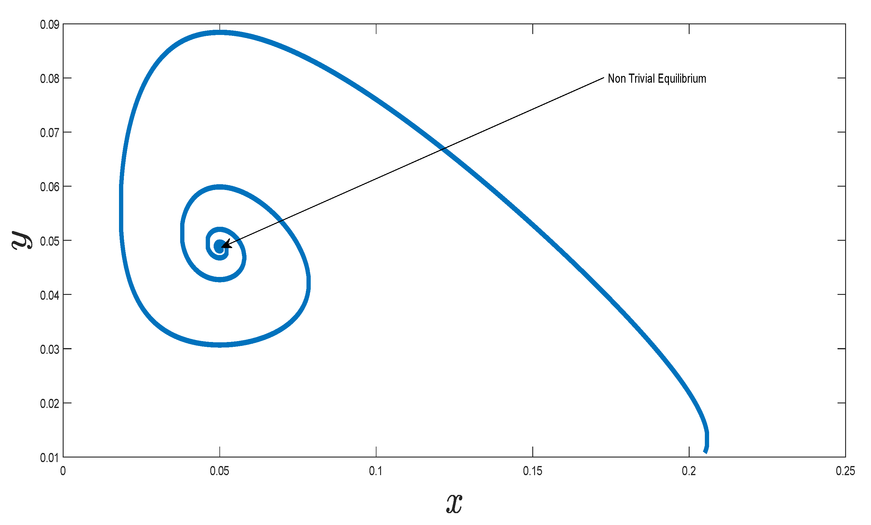
We illustrate the numerical discretizations of the predator–prey model described in the previous section. For the graphical representations, we consider different contexts by considering the different values of the parameters of the model. We, firstly, analyze the solution according to the fixed harvesting rate (case 1). In first cases, we fix the following assumptions [53]: the growth rate r = 0.03 and the carrying capacity k = 0.25 , the rate of predation is a = 0.5 , the efficiency of predation is c = 0.4 , d = 0.01 is death rate of the predator species and γ = 0.95 is the order. In the first subcase, we fix the harvesting rate as h = 0.00033 ; in Figure 1, we depict the evolutions of the predator and the prey species in time. We notice the trajectory describes a cycle and converges to the non-trivial equilibrium point.
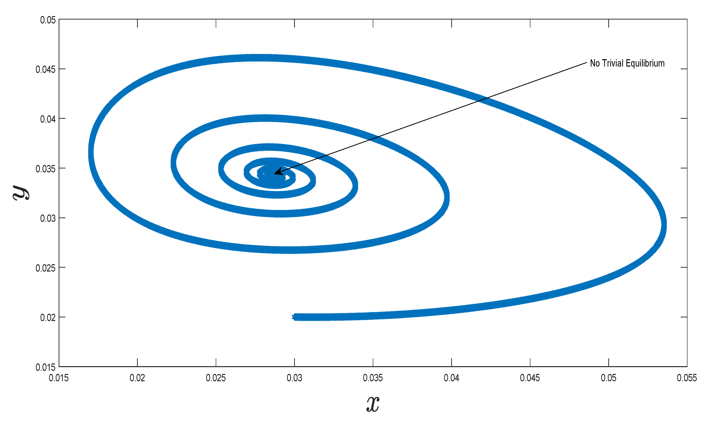
In Figure 2, we depict the dynamics of the P–PM under no harvesting rate ( h = 0 ) . We notice the same dynamics as in the presence of harvesting rate; the solutions describe a cycle and converge to a non-trivial equilibrium point.
We notice when the harvesting rate varies and exceeds h = 0.00035 , in Figure 3, we see the line instead of the cycle. It corresponds that the non-trivial equilibrium point is not stable. Furthermore, the obtained solutions for the predator–prey model are unrealistic, since the species can not be negative; they do not make sense.
In conclusion, the harvesting rate has a significant impact on the dynamics of the P–PMs. We note after certain values that the behaviors of the solutions are in contradiction with the real possible phenomena. Thus, it is crucial to control the harvesting rate into the predator–prey models. There exist many methods to control it, such as the maximization principle using the Hamiltonian approach. This problem is not addressed in this paper.
Let us give illustrative results to support our results. We change the values of the parameters, and we suppose the following assumptions [53]: the growth rate r = 0.004 and the carrying capacity k = 0.25 , the rate of predation a = 0.1 , the efficiency of predation c = 0.4 , the death rate of the predator species d = 0.001 , the harvesting rate h = 0.000005 and the order is maintained at γ = 0.95 .
We notice in Figure 4 that the evolutions of the predator and the prey species have been depicted in time. We see the trajectory describes a cycle and converges to the non-trivial equilibrium point. In conclusion, after variation in the parameters, the solutions respect the cycles; there are not many changes in the behaviors of the solutions. Our fractional model is, in general, stable but strongly depends on the values of the harvesting rate, because when the harvesting rate value exceeds certain values, the cycle is displayed.
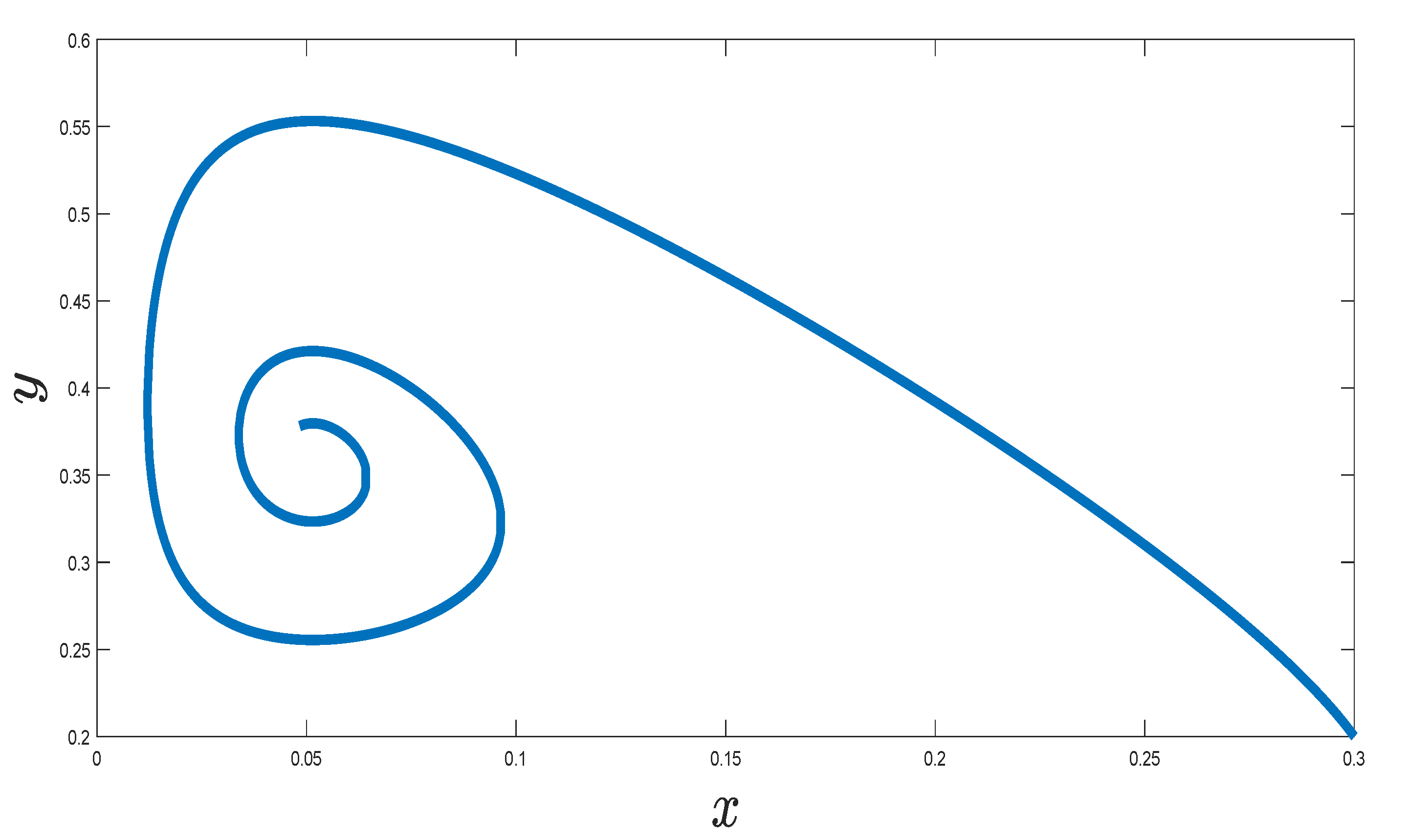
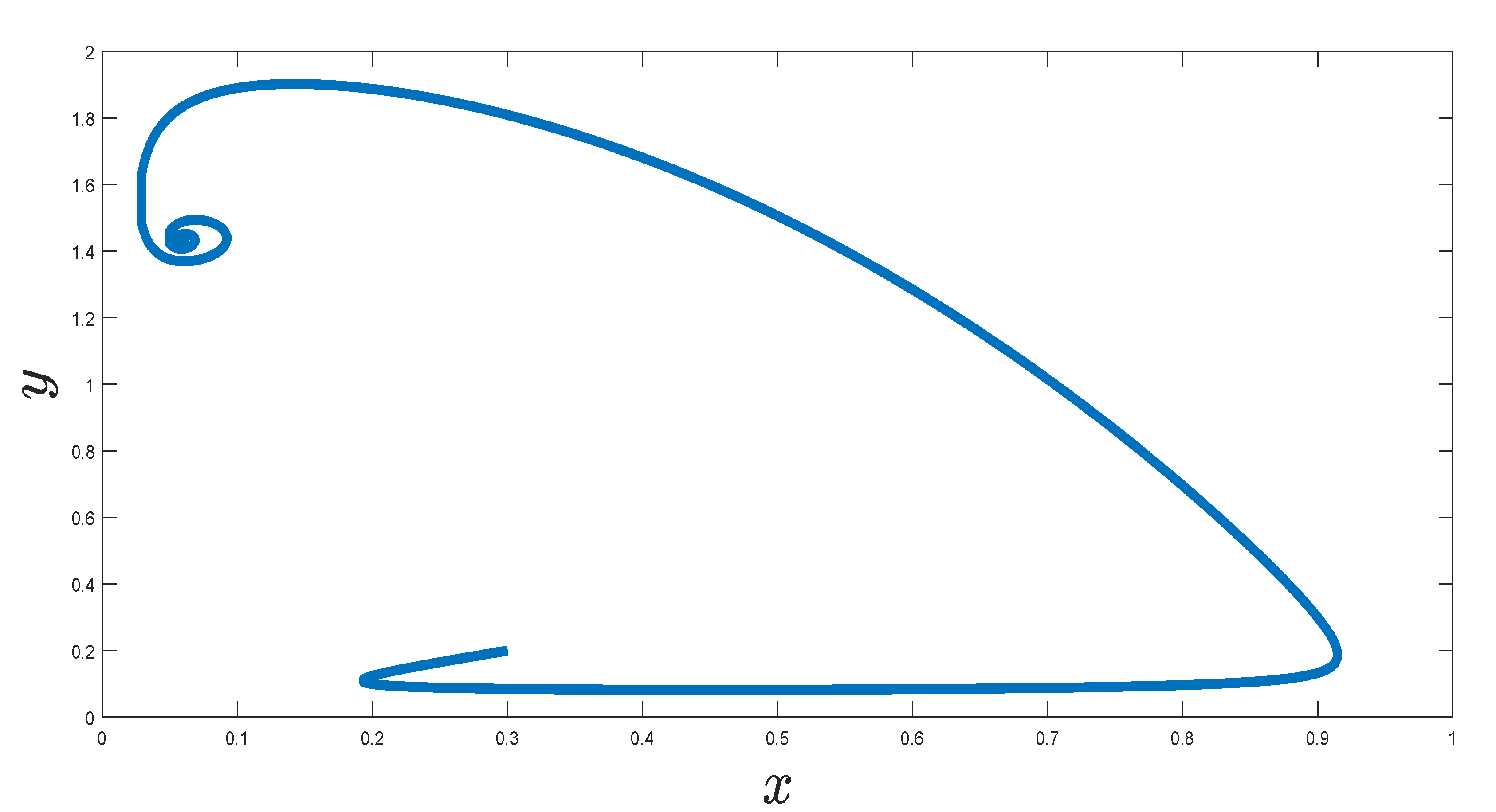
To support our numerical scheme, we consider the second case where the harvesting rate is expressed as the linear representation of the predator population, i.e., h = m y . We set the following assumptions [53]: the growth rate r = 0.1 and the carrying capacity k = 0.5 , a = 0.25 represents the rate of predation, c = 0.8 denotes the efficiency of predation, d = 0.01 is death rate of the predator species, the order γ = 0.95 and m = 0.0003 . In Figure 5, we represent graphically the dynamics of the predator versus prey.
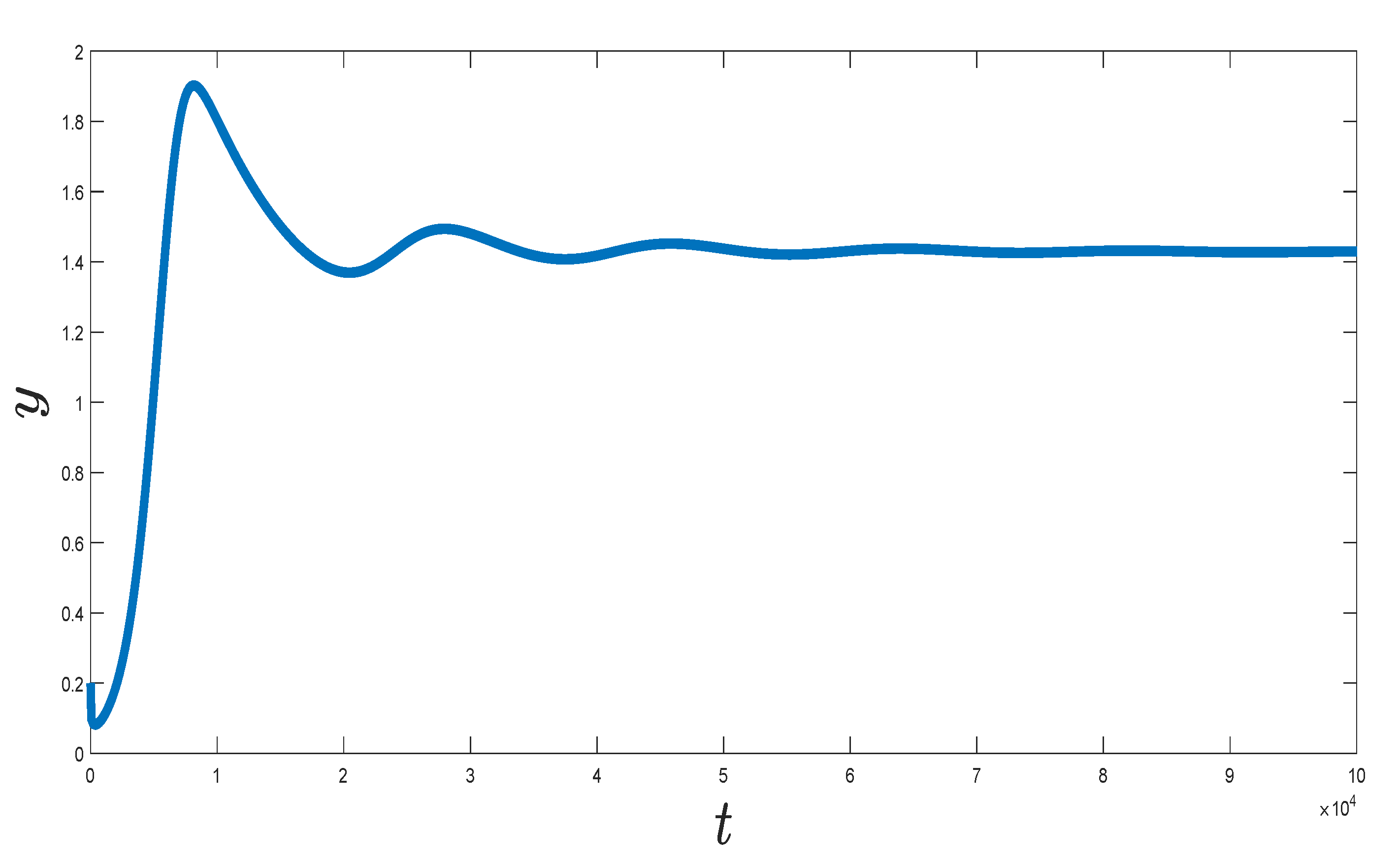
In Figure 6, we represent graphically the dynamics of the predator in time.
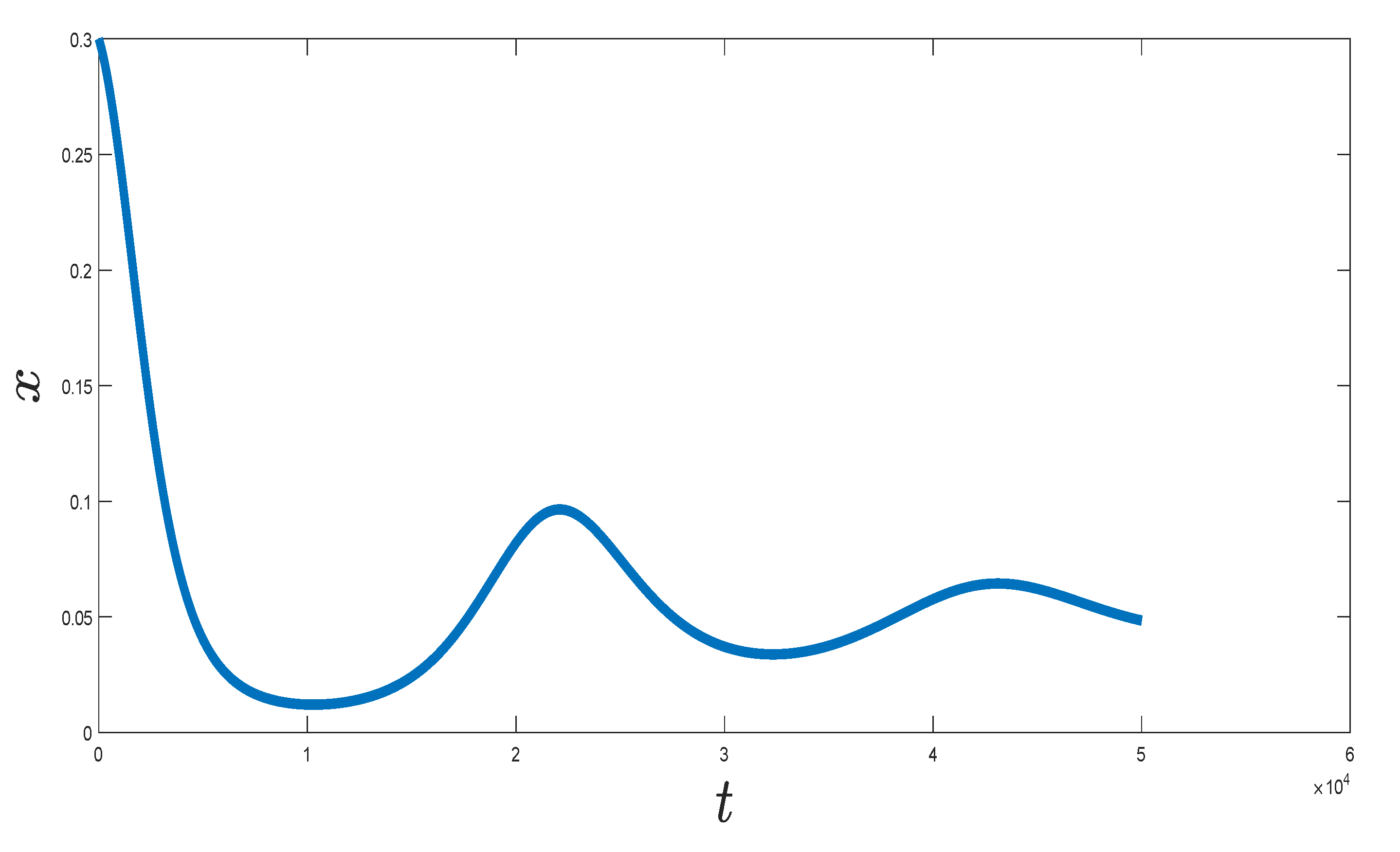
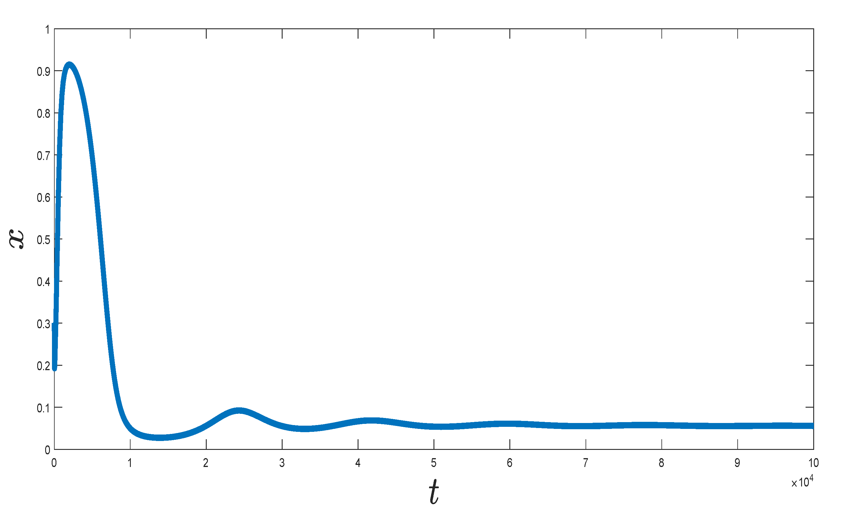
In Figure 7, we represent graphically the dynamics of the prey in time.
In the figures of the first case, the order converges to the classical order, i.e., to 1. We now depict the figures when the order is arbitrary in the interval ( 0 , 1 ) which we consider it as γ = 0.85 . In Figure 8, we represent graphically the dynamics of the predator versus the prey.
In Figure 9, we represent graphically the dynamics of the predator in time.
In Figure 10, we represent graphically the dynamics of the prey in time.
We notice by comparing the plots in Figure 6, Figure 7, Figure 9 and Figure 10 that the fractional order derivative has a significant impact on the dynamics of the suggested predator–prey model represented by Equation (11). In general, it has an acceleration effect on the model process. It is remarkable that the model has not been previously considered in terms of fractional derivatives. For this reason, making a comparison of it with those existing in the literature is a bit difficult. A possible comparison can be done with the prey–predator model which was constructed by integer-order derivative in [53]. In terms of comparison we notice that the fractional order derivative generates an acceleration effect in the dynamics. These mentioned differences can be seen when looking at the comparisons of Figure 6 and Figure 9; Figure 7 and Figure 10.

8. Concluding Remarks

In this paper, modeling and analysis of the fractional order P–PM which contains the harvesting rate have been provided. Since the harvesting rate has a significant impact on the dynamics of the predator–prey models, we have demonstrated after certain values, the behaviors of the solutions are in contradiction with the real possible phenomena. Moreover, the basic reproduction number R 0 has been computed by the next generation matrix method which performs as a threshold parameter in the disease transmission and determines whether the disease persists or vanishes from the population. The existence and uniqueness of the solutions of the proposed fractional system have been examined. Additionally, the stability conditions of the equilibrium points for the fractional system have been discussed. Meanwhile, the global dynamics of the equilibria have been obtained by the Lyapunov functional approach method. It is well-known that the infection spreads in the population when R 0 > 1 . A new numerical algorithm based on the numerical discretization of the Riemann–Liouville integral has been introduced and it has been successfully applied for the corresponding numerical solution of the proposed predator–prey fractional-order model to carry out the numerical simulations for different values of the fractional order γ . The model introduced in the paper is new in the context of fractional order derivatives; therefore, to analyze the dynamics of the predator and prey, we need to get the solutions to the proposed model. Since it is straightforward that the analytical solution to the proposed model is not possible, an alternative way to deal with this issue is to construct the numerical scheme. This is because we used an effective and accurate numerical scheme including the discretization of the Riemann–Liouville integral, and by using this scheme, we have managed to obtain numerical solutions to the aforementioned problem. Finally, it has been demonstrated that physical processes are better described using the derivative of fractional order which is more accurate and reliable in comparison with the classical order case. Hence, we replace the integer order time derivative with the Caputo type fractional order derivative.

Author Contributions

Conceptualization, M.Y. and N.S.; methodology, M.Y. and N.S.; investigation, M.Y. and N.S.; writing—original draft preparation, N.S.; writing—review and editing, M.Y. All authors have read and agreed to the published version of the manuscript.

Funding

This research received no external funding.

Acknowledgments

M. Yavuz was supported by TUBITAK (The Scientific and Technological Research Council of Turkey). The authors would like to thank the reviewers for their thoughtful comments and careful efforts towards improving our manuscript.

Conflicts of Interest

The authors declare no conflict of interest.

References

  1. Podlubny, I. Fractional Differential Equations. In Mathematics in Science and Engineering; Academic Press: New York, NY, USA, 1999; Volume 198. [Google Scholar]
  2. Samko, S.G.; Kilbas, A.A.; Marichev, O.I. Fractional Integrals and Derivatives; Gordon and Breach Science Publishers: Yverdon Yverdon-les-Bains, Switzerland, 1993; Volume 1. [Google Scholar]
  3. Katugampola, U.N. New approach to a generalized fractional integral. Appl. Math. Comput. 2011, 218, 860–865. [Google Scholar] [CrossRef] [Green Version]
  4. Caputo, M.; Fabrizio, M. A new definition of fractional derivative without singular kernel. Progr. Fract. Differ. Appl. 2015, 1, 1–15. [Google Scholar]
  5. Atangana, A.; Baleanu, D. New fractional derivatives with non-local and non-singular kernel theory and application to heat transfer model. arXiv 2016, arXiv:1602.03408. [Google Scholar]
  6. Wang, X.; Wang, Z. Dynamic Analysis of a Delayed Fractional-Order SIR Model with Saturated Incidence and Treatment Functio. Int. J. Bifurc. Chaos 2018, 28, 1850180. [Google Scholar] [CrossRef]
  7. Yavuz, M.; Bonyah, E. New approaches to the fractional dynamics of schistosomiasis disease model. Phys. A Stat. Mech. Its Appl. 2019, 525, 373–393. [Google Scholar] [CrossRef]
  8. Ucar, S.; Ucar, E.; Ozdemir, N.; Hammouch, Z. Mathematical analysis and numerical simulation for a smoking model with Atangana–Baleanu derivative. Chaos Solitons Fractals 2019, 118, 300–306. [Google Scholar] [CrossRef]
  9. Jajarmi, A.; Ghanbari, B.; Baleanu, D. A new and efficient numerical method for the fractional modelling and optimal control of diabetes and tuberculosis co-existence. Chaos 2019, 29, 093111. [Google Scholar] [CrossRef]
  10. Naik, P.A.; Yavuz, M.; Zu, J. The Role of Prostitution on HIV Transmission with Memory: A Modeling Approach. Alex. Eng. J. 2020. [Google Scholar] [CrossRef]
  11. Yavuz, M.; Ozdemir, N. Analysis of an Epidemic Spreading Model with Exponential Decay Law. Math. Sci. Appl. E Notes 2020, 8, 142–154. [Google Scholar] [CrossRef] [Green Version]
  12. Sene, N. Stokes’ first problem for heated flat plate with Atangana–Baleanu fractional derivative. Chaos Solitons Fractals 2018, 117, 68–75. [Google Scholar] [CrossRef]
  13. Sene, N. Integral Balance Methods for Stokes’ First, Equation Described by the Left Generalized Fractional Derivative. Physics 2019, 1, 15. [Google Scholar] [CrossRef] [Green Version]
  14. Sene, N. Second-grade fluid model with Caputo-Liouville generalized fractional derivative. Chaos Solitons Fractals 2020, 133, 109631. [Google Scholar] [CrossRef]
  15. Ozarslan, R.; Bas, E.; Baleanu, D.; Acay, B. Fractional physical problems including wind-influenced projectile motion with Mittag-Leffler kernel. AIMS Math. 2020, 5, 467. [Google Scholar] [CrossRef]
  16. Kumar, D.; Singh, J.; Tanwar, K.; Baleanu, D. A new fractional exothermic reactions model having constant heat source in porous media with power, exponential and Mittag-Leffler laws. Int. J. Heat Mass Transf. 2019, 138, 1222–1227. [Google Scholar] [CrossRef]
  17. Yavuz, M.; Ozdemir, N. European vanilla option pricing model of fractional order without singular kernel. Fractal Fract. 2018, 2, 3. [Google Scholar] [CrossRef] [Green Version]
  18. Yavuz, M.; Ozdemir, N. A different approach to the European option pricing model with new fractional operator. Math. Model. Nat. Phenom. 2018, 13, 12. [Google Scholar] [CrossRef] [Green Version]
  19. Sene, N. Analytical solutions and numerical schemes of certain generalized fractional diffusion models. Eur. Phys. J. Plus 2019, 134, 199. [Google Scholar] [CrossRef]
  20. Qureshi, S.; Yusuf, A.; Ali Shaikh, A.; Inc, M.; Baleanu, D. Mathematical modeling for adsorption process of dye removal nonlinear equation using power law and exponentially decaying kernels. Chaos Interdiscip. J. Nonlinear Sci. 2020, 30, 043106. [Google Scholar] [CrossRef]
  21. Owolabi, K.M.; Atangana, A. On the formulation of Adams-Bashforth scheme with Atangana-Baleanu-Caputo fractional derivative to model chaotic problems. Chaos 2019, 29, 023111. [Google Scholar] [CrossRef]
  22. Bhatter, S.; Mathur, A.; Kumar, D.; Nisar, K.S.; Singh, J. Fractional modified Kawahara equation with Mittag-Leffler law. Chaos Solitons Fractals 2020, 131, 109508. [Google Scholar] [CrossRef]
  23. Usta, F. A conformable calculus of radial basis functions and its applications. Int. J. Optim. Control. Theor. Appl. (IJOCTA) 2018, 8, 176–182. [Google Scholar] [CrossRef]
  24. Yavuz, M. Characterization of two different fractional operators without singular kernel. Math. Model. Nat. Phenom. 2019, 14, 302. [Google Scholar] [CrossRef] [Green Version]
  25. Yildiz, T.A.; Jajarmi, A.; Yıldız, B.; Baleanu, D. New aspects of time fractional optimal control problems within operators with nonsingular kernel. Discret. Contin. Dyn. Syst. S 2020, 13, 407–428. [Google Scholar] [CrossRef] [Green Version]
  26. Budak, H.; Usta, F.; Sarikaya, M.Z.; Ozdemir, M.E. On generalization of midpoint type inequalities with generalized fractional integral operators. Revista de la Real Academia de Ciencias Exactas, Físicas y Naturales. Serie A. Matemáticas 2019, 113, 769–790. [Google Scholar] [CrossRef]
  27. Yavuz, M.; Sulaiman, T.A.; Usta, F.; Bulut, H. Analysis and numerical computations of the fractional regularized long-wave equation with damping term. Math. Methods Appl. Sci. 2020. [Google Scholar] [CrossRef]
  28. Özkan, Y.S.; Yaşar, E.; Seadawy, A.R. A third-order nonlinear Schrödinger equation: The exact solutions, group-invariant solutions and conservation laws. J. Taibah Univ. Sci. 2020, 14, 585–597. [Google Scholar] [CrossRef]
  29. Yavuz, M.; Yaşkıran, B. Conformable Derivative Operator in Modelling Neuronal Dynamics. Appl. Appl. Math. 2018, 13, 803–817. [Google Scholar]
  30. Jena, R.M.; Chakraverty, S.; Yavuz, M. Two-hybrid techniques coupled with an integral transform for caputo time-fractional Navier-Stokes Equations. Prog. Fract. Differ. Appl. 2020, 6, 201–213. [Google Scholar]
  31. Ahmad, H.; Seadawy, A.R.; Khan, T.A.; Thounthong, P. Analytic approximate solutions for some nonlinear Parabolic dynamical wave equations. J. Taibah Univ. Sci. 2020, 14, 346–358. [Google Scholar] [CrossRef] [Green Version]
  32. Yavuz, M. Dynamical behaviors of separated homotopy method defined by conformable operator. Konuralp J. Math. 2019, 7, 1–6. [Google Scholar]
  33. Avci, D.; Yavuz, M.; Özdemir, N. Fundamental solutions to the Cauchy and Dirichlet problems for a heat conduction equation equipped with the Caputo-Fabrizio differentiation. In Heat Conduction: Methods, Applications and Research; Nova Science Publishers: Hauppauge, NY, USA, 2019; pp. 95–107. [Google Scholar]
  34. Arnous, A.H.; Seadawy, A.R.; Alqahtani, R.T.; Biswas, A. Optical solitons with complex Ginzburg–Landau equation by modified simple equation method. Optik 2017, 144, 475–480. [Google Scholar] [CrossRef]
  35. Yavuz, M.; Yokus, A. Analytical and numerical approaches to nerve impulse model of fractional-order. Numer. Methods Partial. Differ. Equ. 2020. [Google Scholar] [CrossRef]
  36. Selima, E.S.; Seadawy, A.R.; Yao, X. The nonlinear dispersive Davey-Stewartson system for surface waves propagation in shallow water and its stability. Eur. Phys. J. Plus 2016, 131, 1–16. [Google Scholar] [CrossRef]
  37. Yavuz, M.; Özdemir, N. New numerical techniques for solving fractional partial differential equations in conformable sense. In Non-Integer Order Calculus and Its Applications; Springer: Cham, Switzerland, 2019; pp. 49–62. [Google Scholar]
  38. Seadawy, A.R.; Jun, W. Mathematical methods and solitary wave solutions of three-dimensional Zakharov-Kuznetsov-Burgers equation in dusty plasma and its applications. Results Phys. 2017, 7, 4269–4277. [Google Scholar]
  39. Naik, P.A.; Zu, J.; Ghoreishi, M. Estimating the approximate analytical solution of HIV viral dynamic model by using homotopy analysis method. Chaos Solitons Fractals 2020, 131, 109500. [Google Scholar] [CrossRef]
  40. Yavuz, M. Novel recursive approximation for fractional nonlinear equations within Caputo-Fabrizio operator. In ITM Web of Conferences; EDP Sciences: Jules, France, 2018; Volume 22, p. 01008. [Google Scholar]
  41. Naik, P.A.; Zu, J.; Owolabi, K.M. Modeling the mechanics of viral kinetics under immune control during primary infection of HIV-1 with treatment in fractional order. Phys. A Stat. Mech. Its Appl. 2020, 545, 123816. [Google Scholar] [CrossRef]
  42. Avci, D.; Ozdemir, N.; Yavuz, M. Fractional Optimal Control of Diffusive Transport Acting on a Spherical Region. In Methods of Mathematical Modelling: Fractional Differential Equations; CRC Press: Boca Raton, FL, USA, 2019; p. 63. [Google Scholar]
  43. Seadawy, A.R.; El-Rashidy, K. Dispersive solitary wave solutions of Kadomtsev-Petviashvili and modified Kadomtsev-Petviashvili dynamical equations in unmagnetized dust plasma. Results Phys. 2018, 8, 1216–1222. [Google Scholar] [CrossRef]
  44. Yavuz, M.; Özdemir, N.; Baskonus, H.M. Solutions of Partial Differential Equations Using the Fractional Operator Involving Mittag-Leffler Kernel. Eur. Phys. J. Plus 2018, 133, 215. [Google Scholar] [CrossRef]
  45. Tukur, A.S.; Yavuz, M.; Bulut, H.; Baskonus, H.M. Investigation of the Fractional Coupled Viscous Burger’s Equation Involving Mittag-Leffler Kernel. Phys. A Stat. Mech. Its Appl. 2019, 527, 121126. [Google Scholar]
  46. Iqbal, M.; Seadawy, A.R.; Lu, D. Construction of solitary wave solutions to the nonlinear modified Kortewege-de Vries dynamical equation in unmagnetized plasma via mathematical methods. Mod. Phys. Lett. A 2018, 33, 1850183. [Google Scholar] [CrossRef]
  47. Keten, A.; Yavuz, M.; Baleanu, D. Nonlocal cauchy problem via a fractional operator involving power kernel in Banach spaces. Fractal Fract. 2019, 3, 27. [Google Scholar] [CrossRef] [Green Version]
  48. Helal, M.A.; Seadawy, A.R.; Zekry, M.H. Stability analysis of solitary wave solutions for the fourth-order nonlinear Boussinesq water wave equation. Appl. Math. Comput. 2014, 232, 1094–1103. [Google Scholar] [CrossRef]
  49. Sulaiman, T.A.; Bulut, H.; Yokus, A.; Baskonus, H.M. On the exact and numerical solutions to the coupled Boussinesq equation arising in ocean engineering. Indian J. Phys. 2019, 93, 647–656. [Google Scholar] [CrossRef]
  50. Evirgen, F.; Yavuz, M. An alternative approach for nonlinear optimization problem with Caputo-Fabrizio derivative. In ITM Web of Conferences; EDP Sciences: Jules, France, 2018; Volume 22, p. 01009. [Google Scholar]
  51. Fahd, J.; Abdeljawad, T.; Baleanu, D. On the generalized fractional derivatives and their Caputo modification. J. Nonlinear Sci. Appl. 2017, 10, 2607–2619. [Google Scholar]
  52. Kilbas, A.A.; Srivastava, H.M.; Trujillo, J.J. Theory and Applications of Fractional Differential Equations. In North-Holland Mathematics Studies; Elsevier: Amsterdam, The Netherlands, 2006; Volume 204. [Google Scholar]
  53. Li, B.; Liu, S.; Cui, J.; Li, J. A Simple Predator-Prey Population Model with Rich Dynamics. Appl. Sci. 2016, 6, 151. [Google Scholar] [CrossRef]
  54. Dubey, B. A Prey-Predator Model with a Reserved Area. Nonlinear Anal. Model. Control 2007, 12, 479–494. [Google Scholar] [CrossRef]
  55. Seo, G.; DeAngelis, D.L. A Predator-Prey Model with a Holling Type I Functional Response Including a Predator Mutual Interference. J. Nonlinear Sci. 2013, 21, 811–833. [Google Scholar] [CrossRef]
  56. Suryanto, A.; Darti, I.; Panigoro, H.S.; Kilicman, A. A Fractional-Order Predator–Prey Model with Ratio-Dependent Functional Response and Linear Harvesting. Mathematics 2019, 7, 1100. [Google Scholar] [CrossRef] [Green Version]
  57. Tang, B. Dynamics for a fractional-order predator-prey model with group defense. Sci. Rep. 2020, 10, 4906. [Google Scholar] [CrossRef]
  58. Elettreby, M.F.; Al-Raezah, A.A.; Nabil, T. Fractional-Order Model of Two-Prey One-Predator System. Math. Probl. Eng. 2017, 2017, 6714538. [Google Scholar] [CrossRef] [Green Version]
  59. Liu, Y.; Xin, B. Numerical Solutions of a Fractional Predator-Prey System. Adv. Differ. Equ. 2011, 2011, 1–11. [Google Scholar] [CrossRef] [Green Version]
  60. Lv, Y.; Yuan, R.; Pei, Y. A prey-predator model with harvesting for fishery resource with reserve area. Appl. Math. Model. 2013, 37, 3048–3062. [Google Scholar] [CrossRef]
  61. Heggeru, C.M.; Lan, K. Local stability analysis of ratio-dependent predator–prey models with predator harvesting rates. Appl. Math. Comput. 2015, 270, 349–357. [Google Scholar]
  62. Kar, T.K. Selective harvesting in a predator-prey fishery with time delay. Math. Comput. Model. 2003, 38, 449–458. [Google Scholar] [CrossRef]
  63. Javidi, M.; Nyamoradi, N. Dynamic analysis of a fractional order prey-predator interaction with harvesting. Appl. Math. Model. 2013, 37, 8946–8956. [Google Scholar] [CrossRef]
  64. Huanga, J.; Ruan, S.; Song, J. Bifurcations in a predator-prey system of Leslie type with generalized Holling typeIII functional response. J. Differ. Equ. 2014, 257, 1721–1752. [Google Scholar] [CrossRef]
  65. Rebaza, J. Dynamics of prey threshold harvesting and refuge. J. Comput. Appl. Math. 2012, 236, 1743–1752. [Google Scholar] [CrossRef] [Green Version]
  66. Bulai, I.M.; Hilker, F.M. Eco-epidemiological interactions with predator interference and infection. Theor. Popul. Biol. 2019, 130, 191–202. [Google Scholar] [CrossRef]
  67. Laurie, H.; Venturino, E.; Bulai, I.M. Herding induced by encounter rate, with predator pressure influencing prey response. In Current Trends in Dynamical Systems in Biology and Natural Sciences; Springer: Cham, Switzerland, 2020; pp. 63–93. [Google Scholar]
  68. Matignon, D. Stability results on fractional differential equations to control processing. In Proceedings of the Computational Engineering in Syatems and Application Multiconference, Lille, France, 9–12 July 1996; IMACS, IEEE-SMC: Lille, France, 1996; Volume 2, pp. 963–968. [Google Scholar]
  69. Sene, N. Stability analysis of the generalized fractional differential equations with and without exogenous inputs. J. Nonlinear Sci. Appl. 2019, 12, 562–572. [Google Scholar] [CrossRef]
  70. Seo, G.; Kot, M. A comparison of two predator–prey models with Holling’s type I functional response. Math. Biosci. 2008, 212, 161–179. [Google Scholar] [CrossRef]
  71. Murdoch, W.W.; Briggs, C.J.; Nisbet, R.M. Consumer-Resource Dynamics; Princeton University Press: Princeton, NJ, USA, 2003; Volume 36. [Google Scholar]
  72. Lin, W. Global existence theory and chaos control of fractional differential equations. J. Math. Anal. Appl. 2007, 332, 709–726. [Google Scholar] [CrossRef] [Green Version]
  73. Garrappa, R. Numerical solution of fractional differential equations: A survey and a software tutorial. Mathematics 2018, 6, 16. [Google Scholar] [CrossRef] [Green Version]
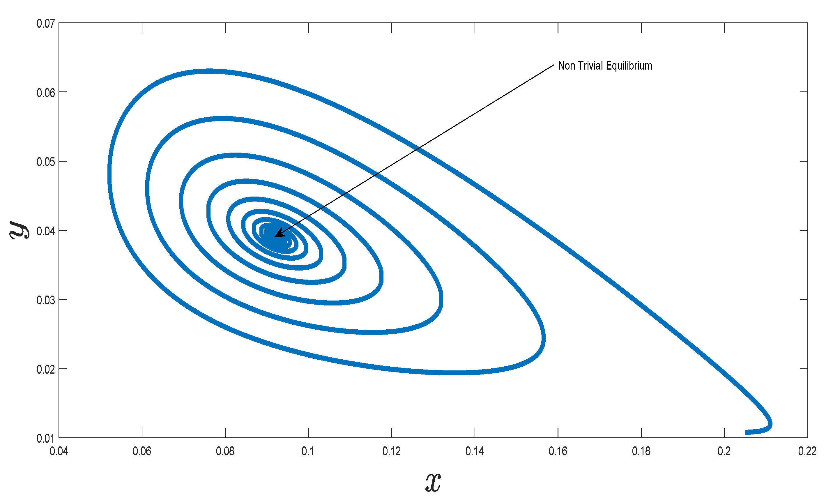
Figure 1. Phase diagram of fractional P–PM with γ = 0.95 .
Fractalfract 04 00035 g001
Figure 2. Dynamical behavior of fractional P–PM under no harvesting rate with γ = 0.95 .
Fractalfract 04 00035 g002
Figure 3. Dynamical behavior of fractional P–PM with γ = 0.95 .
Fractalfract 04 00035 g003
Figure 4. Dynamical behavior of fractional P–PM with γ = 0.95 .
Fractalfract 04 00035 g004
Figure 5. Dynamics of the predator and prey in the model for γ = 0.95 .
Fractalfract 04 00035 g005
Figure 6. Dynamics of the predator in the model for γ = 0.95 .
Fractalfract 04 00035 g006
Figure 7. Dynamics of the prey in the model for γ = 0.95 .
Fractalfract 04 00035 g007
Figure 8. Dynamics of the predator and prey in the model for γ = 0.85 .
Fractalfract 04 00035 g008
Figure 9. Dynamics of the predator in the model for γ = 0.85 .
Fractalfract 04 00035 g009
Figure 10. Dynamics of the prey in the model for γ = 0.85 .
Fractalfract 04 00035 g010