Random Variables and Stable Distributions on Fractal Cantor Sets

Abstract

In this paper, we introduce the concept of fractal random variables and their related distribution functions and statistical properties. Fractal calculus is a generalisation of standard calculus which includes function with fractal support. Here we combine this emerging field of study with probability theory, defining concepts such as Shannon entropy on fractal thin Cantor-like sets. Stable distributions on fractal sets are suggested and related physical models are presented. Our work is illustrated with graphs for clarity of the results.

1. Introduction

Fractals are geometrical shapes such that their fractal dimensions are more than their topological dimensions; they have self-similar properties and are scale invariant [1,2,3,4,5,6]. Analysis on sets, vector spaces, and manifolds plays an important role in physics, including in classical mechanics, quantum mechanics, and general relativity. Recently, probability, measure theory, fractional spaces, and fractional calculus have been used to build a theory of analysis on fractals [7,8,9,10,11,12,13,14,15,16,17,18,19,20].

Fractal calculus was introduced in the seminal papers [21,22,23,24] where it was originally applied for functions on fractal sets and curves. This new framework, known as $F^{\alpha }$-calculus or $F^{\alpha }$-C, is simple, algorithmic, and local. It has a natural geometrical meaning: The order of the derivatives is equal to the dimension of the sets on which the function is defined. The locality of this framework is important in physics, since measurements are local in physics and do not violate causality principles. It also has physical meaning, since the $\gamma$-dimension and spectral dimension are connected to the physical properties of fractals. In addition, the conjugacy of $F^{\alpha }$-C between standard calculus leads to the same properties, such as Leibniz’s rule and the chain rule for derivatives [21,22,23,24,25,26,27].

After its introduction in the papers cited above, fractal calculus has been applied in optics, classical mechanics, electromagnetics, and quantum mechanics. Random walks on fractal sets and the corresponding mean square displacements have been modelled by fractal calculus [28,29,30,31,32,33,34,35]. Non-local analogues of fractional derivatives have been defined as a model for processes on fractal sets with memory effect [36].

Shannon entropy has many applications in science and in engineering, especially information theory, where it may be used to estimate the average minimum number of bits necessary to encode a string of symbols represented by frequencies. Applying Shannon entropy to continuous probability spaces is not straightforward [37,38]. Shannon wavelets and their fractional derivatives were examined in [39,40,41].

Continuing the research along these lines, in the current work we define fractal random variables and fractal stable distributions on thin Cantor-like sets. We analyse several examples of fractal random variables and fractal distributions, and we explain physical models for fractal stable distributions. Shannon entropy on totally discontinuous fractal sets is defined, which can also give the continuum cases.

The plan of the paper is as follows. We introduce preliminaries for the paper in Section 2. In Section 3 we define fractal random variables and distributions on thin Cantor-like sets, with various related features, illustrated with several examples. In Section 4 we define what it means for a fractal distribution to be stable, and present different kinds of stable distributions on fractal sets. Section 5 analyses a related physical model, and Section 6 is devoted to giving the conclusions. Section 2 consists of review material concerning the existing theory of fractal calculus, while Section 3, Section 4 and Section 5 contain our original research in this direction.

2. Basic Tools and Prerequisites

In this section, we give a brief summary of fractal calculus which is a generalisation of standard calculus on Euclidean space.

One of the most fundamental fractal sets is the middle-$\mathit{\beta }$ Cantor set, which is defined for any $1<\beta <\infty$ by applying the following algorithm [42]:

1.

Delete an open interval of length $(1/\beta )$ from the middle of $I=[0,1]$.

2.

Remove an open interval of length $(1/\beta )$ from the middle of each disjoint closed interval remaining after step 1.

⋮

k. 

Remove an open interval of length $(1/\beta )$ from the middle of each disjoint closed interval remaining after step $k-1$.

Applying this algorithm for infinitely many steps yields the thin Cantor-like set which is called the middle-$\beta$ Cantor set, and which we denote by $C^{\beta }$. The Hausdorff dimension of this set, as defined in [5,42], is

$$D_H\left(C^{\beta }\right)=\frac{log\left(2\right)}{log\left(2\right)-log(1-\beta )}.$$

(1)

In Figure 1a we illustrate the algorithm mentioned above for establishing the middle-$\beta$ Cantor set.

For a middle-$\beta$ Cantor set, the flag function is defined [21,22] as follows

$$\Lambda (C^{\beta },J)=\left\{\begin{array}{c}1\mathrm{if}{C}^{\beta }\cap J\ne \varnothing \hfill \\ 0\mathrm{otherwise}.\hfill \end{array}\right.$$

(2)

where $J=[a_1,a_2]$ is an interval and $Q_{[a_1,a_2]}=\{a_1=t_0,t_1,t_2,\cdots ,t_n=a_2\}$ is a subdivision of J.

Then, for any $\eta \in (0,1]$, the quantity ${{\rm Y}}^{\eta }[C^{\beta },J]$ is defined [21,22,26] by

$${{\rm Y}}^{\eta }[C^{\beta },J]=\sum _{i=1}^n\Gamma (\eta +1){(t_i-t_{i-1})}^{\eta }\Lambda (C^{\beta },[t_{i-1},t_i]).$$

(3)

The mass function ${\mathcal{K}}^{\eta }(C^{\beta },a_1,a_2)$ is defined [21,22,26] by

$$\begin{array}{ccc}\hfill {\mathcal{K}}^{\eta }(C^{\beta },a_1,a_2)& =& \underset{\delta \to 0}{lim}\left(\underset{J_{[a_1,a_2]}:\left|J\right|\le \delta }{inf}{{\rm Y}}^{\eta }[C^{\beta },J]\right),\hfill \\ & =& \underset{\delta \to 0}{lim}{\mathcal{K}}_{\delta }^{\eta }(C^{\beta },a_1,a_2)\hfill \end{array}$$

(4)

where the infimum is taken over all subdivisions Q of $[a_1,a_2]$ satisfying $\left|J\right|:={max}_{1\le i\le n}(t_i-t_{i-1})\le \delta$ for every $J=[t_{i-1},t_i]$ within Q.

The integral staircase function $S_{C^{\beta }}^{\eta }\left(t\right)$ of order $\eta$ for the fractal set $C^{\beta }$ is defined [21,22] by

$$S_{C^{\beta }}^{\eta }\left(t\right)=\left\{\begin{array}{c}{\mathcal{K}}^{\eta }(C^{\beta },t_0,t)\mathrm{if}t\ge t_0,\hfill \\ -{\mathcal{K}}^{\eta }(C^{\beta },t_0,t)\mathrm{otherwise},\hfill \end{array}\right.$$

(5)

where $t_0$ is a fixed arbitrary real number.

In Figure 1b we plot the integral staircase function for the middle-$\beta$ Cantor set by letting $\beta =2$.

The $\mathit{\gamma }$-dimension of $C^{\beta }\cap [a_1,a_2]$ is

$$\begin{array}{cc}\hfill {dim}_{\gamma }(C^{\beta }\cap [a_1,a_2])& =inf\{\eta :{\mathcal{K}}^{\eta }(C^{\beta },a_1,a_2)=0\}\hfill \\ & =sup\{\eta :{\mathcal{K}}^{\eta }(C^{\beta },a_1,a_2)=\infty \}.\hfill \end{array}$$

(6)

We use the notation $\alpha =\alpha \left(\beta \right)$ to denote the $\gamma$-dimension of the fractal set $C^{\beta }$. The $\gamma$-dimension of the middle-$\beta$ Cantor set is equal to its Hausdorff dimension $D_H\left(C^{\beta }\right)$ given by Equation (1) [21,22], so we have the following expression for the function $\alpha \left(\beta \right)$

$$\alpha \left(\beta \right)=\frac{log\left(2\right)}{log\left(2\right)-log(1-\beta )}.$$

(7)

Figure 1c presents approximate ${\mathcal{K}}_{{\delta }_2}^{\eta }/{\mathcal{K}}_{{\delta }_1}^{\eta }$, where ${\delta }_2<{\delta }_1$ (specifically, ${\delta }_1=0.1$ and ${\delta }_2=0.8\times {10}^{-4}$).

For a thin Cantor-like set, the fractal characteristic function is defined by

$${\chi }_{C^{\beta }}\left(t\right)=\left\{\begin{array}{cc}\frac{1}{\Gamma (\alpha +1)},\hfill & t\in C^{\beta };\hfill \\ 0,\hfill & \mathrm{o}therwise,\hfill \end{array}\right.$$

(8)

where $\alpha$ is the $\gamma$-dimension defined by Equation (7). In Figure 1d we plot the characteristic function for the thin Cantor-like set by choosing $\beta =2$.

Suppose $h:C^{\beta }\to \Re$ and $t\in C^{\beta }$. Then l is said to be the ${\mathit{C}}^{\mathit{\beta }}$-limit of h, or the limit of h through the points of $C^{\beta }$, as $z\to t$, if we have

$$\left(z\in C^{\beta }\mathrm{and}|z-t|<\delta \right)\Rightarrow |h\left(z\right)-l|<ϵ.$$

(9)

If l exists, then we write this relation as follows

$$l=C_{-}^{\beta }\underset{z\to t}{lim}h\left(z\right).$$

(10)

$C^{\beta }$-continuity. A function $h:C^{\beta }\to \Re$ is defined to be $C^{\beta }$-continuous at $t\in C^{\beta }$ if

$$h\left(t\right)=C_{-}^{\beta }\underset{z\to t}{lim}h\left(z\right).$$

(11)

$C^{\beta }$-differentiation. If $C^{\beta }$ is a $\beta$-perfect set, then the $C^{\beta }$-derivative to order $\eta$ of a function h is defined on $C^{\beta }$ at a point t if the following limit exists [21,22,26]

$$D_{C^{\beta }}^{\eta }h\left(t\right)=\left\{\begin{array}{c}{C}_{-}^{\beta }\underset{z\to t}{lim}\frac{h\left(z\right)-h\left(t\right)}{S_{C^{\beta }}^{\eta }\left(z\right)-S_{C^{\beta }}^{\eta }\left(t\right)},\mathrm{if}z\in C^{\beta },\hfill \\ 0,\mathrm{otherwise}.\hfill \end{array}\right.$$

(12)

$C^{\beta }$-integration. The $C^{\beta }$-integral to order $\eta$ of h on $[a_1,a_2]$ is notated by ${\int }_{a_1}^{a_2}h\left(t\right)d_{C^{\beta }}^{\eta }t$ and is approximately given in [21,22,26] by the following sum

$${\int }_{a_1}^{a_2}h\left(t\right)d_{C^{\beta }}^{\eta }t\approx \sum _{i=1}^n{h}_i\left(t\right)(S_{C^{\beta }}^{\eta }\left(t_j\right)-S_{C^{\beta }}^{\eta }\left(t_{j-1}\right)).$$

(13)

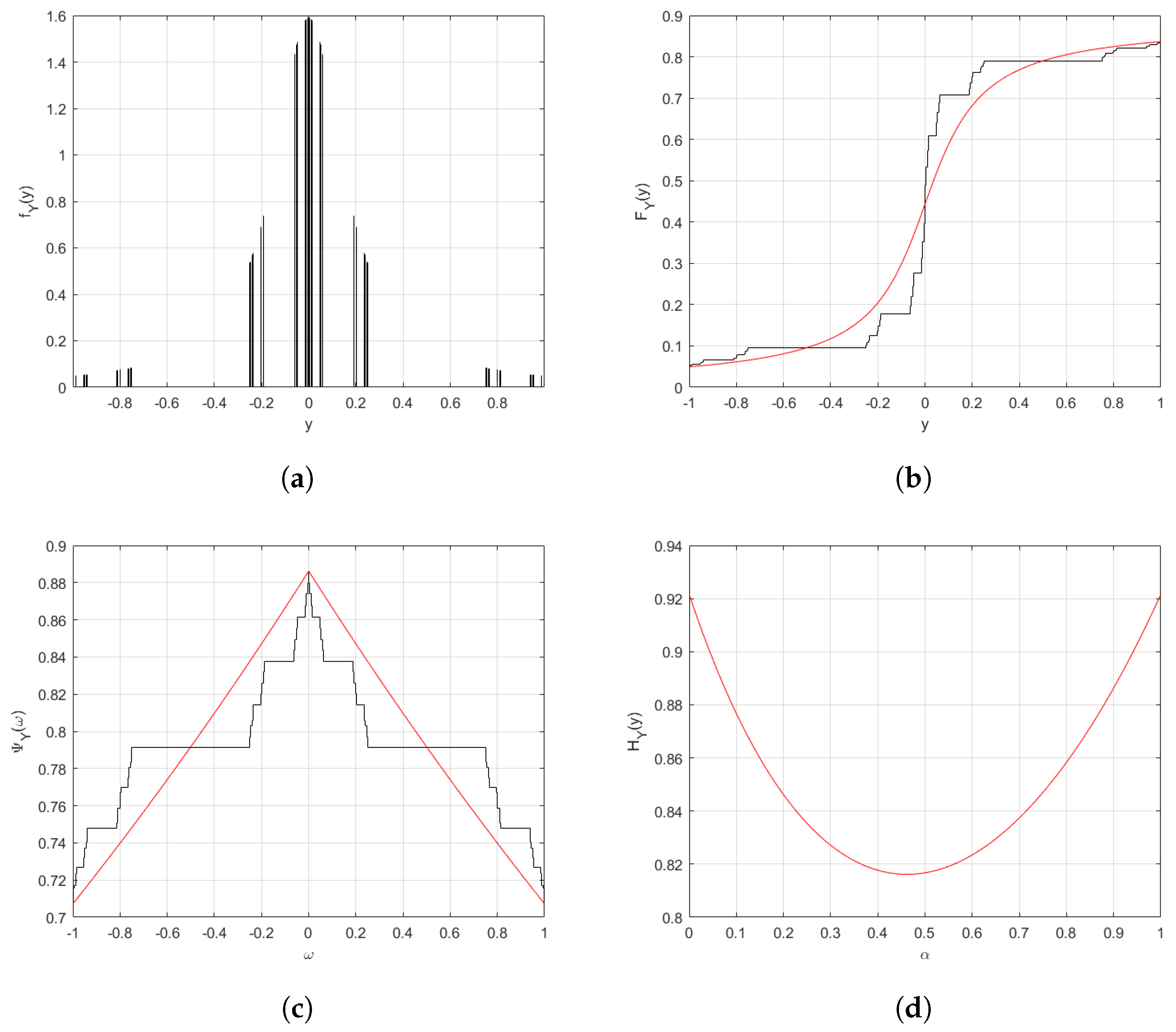
3. Distributions on Thin Cantor-Like Sets

In this section we define random variables and their features on fractals [43,44].

Random variables on fractal sets. A random variable on a thin Cantor-like set, which we shall call an RVC, is defined by a mapping

$$Y\left(\xi \right):\mathcal{S}\to C^{\beta }$$

(14)

where the set $\mathcal{S}$ is the sample space.

Distribution function of an RVC. The distribution function of a random variable Y as above is defined to be

$$F_Y\left(y\right)=P(Y\left(\xi \right)\le y),y\in C^{\beta }.$$

(15)

Probability density function of an RVC. Let $Y\left(\xi \right)$ be an RVC and its distribution function $F_Y\left(y\right)$ be $C^{\beta }$-continuous. The fractal probability density function is defined as

$$f_Y\left(y\right)=D_{C^{\beta }}^{\alpha }{F}_Y\left(y\right),$$

(16)

where $\alpha$ is the $\gamma$-dimension of $C^{\beta }$ as defined in Equation (7). This also gives the relation

$$F_Y\left(y\right)={\int }_{-\infty }^{\infty }{f}_Y\left(y\right)d_{C^{\beta }}^{\alpha }y.$$

(17)

Mean and variance of an RVC. The mean of an RVC Y, denoted by ${\mu }_Y$ or $E\left(Y\right)$, is defined by

$${\mu }_Y={\int }_{-\infty }^{\infty }y{f}_Y\left(y\right)d_{C^{\beta }}^{\alpha }y$$

(18)

The variance of Y, denoted by ${\sigma }_Y^2$ or $Var\left(Y\right)$, is defined by

$${\sigma }_Y^2={\int }_{-\infty }^{\infty }{(y-{\mu }_Y)}^2{f}_Y\left(y\right)d_{C^{\beta }}^{\alpha }y.$$

(19)

Moment of an RVC. For any $m\in \mathbb{N}$, the m-th moment of an RVC Y is defined by

$$E\left(Y^m\right)={\int }_{-\infty }^{\infty }{y}^m{f}_Y\left(y\right)d_{C^{\beta }}^{\alpha }y.$$

(20)

Moment generating function. The moment generating function of an RVC Y is defined by

$$M_Y\left(t\right)=E\left(e^{tY}\right)={\int }_{-\infty }^{\infty }{e}^{ty}{f}_Y\left(y\right)d_{C^{\beta }}^{\alpha }y.$$

(21)

Characteristic function of an RVC. The characteristic function of an RVC Y is defined by

$${\mathsf{\Psi }}_Y\left(\omega \right)={\int }_{-\infty }^{\infty }{e}^{i\omega y}{f}_Y\left(y\right)d_{C^{\beta }}^{\alpha }y,$$

(22)

where $\omega$ is a real number and $i=\sqrt{-1}$.

The fractal Shannon entropy of an RVC. The fractal Shannon entropy (fractal differential entropy) of an RVC Y is defined by

$$H_Y\left(y\right)=-{\int }_Y{f}_Y\left(y\right)log\left(f_Y\left(y\right)\right)d_{C^{\beta }}^{\alpha }y.$$

(23)

Example 1.

Consider a fractal Cauchy random variable Y with parameter a, whose probability density function is as follows:

$$f_Y\left(y\right)=\frac{a}{\pi ({\left(y{\chi }_{C^{\beta }}\right)}^2+a^2)},-\infty <y<+\infty$$

(24)

where $a\in (0,\infty )$ is constant. In Figure 2a we plot this probability density Equation (24).

The distribution function of this fractal Cauchy random variable, by using Equation (17), is

$$F_Y\left(y\right)=\frac{\Gamma (1+\alpha )}{2}+\frac{\Gamma (1+\alpha )}{\pi }arctan\left(\frac{S_{C^{\beta }}^{\alpha }\left(y\right)}{a\Gamma (1+\alpha )}\right),$$

(25)

where again α is the γ-dimension given by Equation (7) of the thin Cantor set $C^{\beta }$ which is a compact set [21]. In Figure 2b we sketch this distribution Equation (25).

Using Equation (22) we have the characteristic function of the fractal Cauchy RVC Y as follows:

$${\mathsf{\Psi }}_Y\left(\omega \right)={\int }_{-\infty }^{\infty }{e}^{i\omega y}\frac{a}{\pi ({\left(y{\chi }_{C^{\beta }}\right)}^2+a^2)}{d}_{C^{\beta }}^{\alpha }y=\Gamma (1+\alpha )e^{-a\left|\frac{S_{C^{\beta }}^{\alpha }\left(\omega \right)}{\Gamma (1+\alpha )}\right|}.$$

(26)

In Figure 2c we show this characteristic Equation (26).

The fractal Shannon entropy of the fractal Cauchy random variable, utilising Equation (23), is

$$\begin{array}{cc}\hfill H_Y\left(y\right)& =-{\int }_{-\infty }^{\infty }\frac{a}{\pi ({\left(y{\chi }_{C^{\beta }}\right)}^2+a^2)}log\left(\frac{a}{\pi ({\left(y{\chi }_{C^{\beta }}\right)}^2+a^2)}\right)d_{C^{\beta }}^{\alpha }y\hfill \\ \hfill & =\Gamma (\alpha +1)log\left(4\pi a\right).\hfill \end{array}$$

(27)

In Figure 2d we draw this Equation (27).

Example 2.

Consider a fractal Laplace random variable Y with the following probability density function

$$f_Y\left(t\right)=\frac{1}{2c}exp\left(-\frac{|t{\chi }_{C^{\beta }}-\nu |}{c}\right),$$

(28)

where $c\in (0,\infty )$ and $\nu \in \Re$ are constant parameters.

This fractal Laplace random variable has distribution function

$$F_Y\left(t\right)=\frac{\Gamma (1+\alpha )}{2}+\frac{\Gamma (1+\alpha )}{2}sgn(t-\nu )\left(1-exp\left(\frac{S_{C^{\beta }}^{\alpha }\left(t\right)-\nu \Gamma (1+\alpha )}{c\Gamma (1+\alpha )}\right)\right),$$

(29)

mean $E\left[Y\right]=\Gamma (1+\alpha )\nu$, variance $Var\left[Y\right]=2{(c\Gamma (1+\alpha ))}^2$, fractal Shannon entropy

$$H_Y\left(t\right)=log(2c\Gamma (1+\alpha )e),$$

(30)

and characteristic function

$${\mathsf{\Psi }}_Y\left(\omega \right)=\frac{\Gamma (1+\alpha )exp\left(\Gamma (1+\alpha )\nu i{S}_{C^{\beta }}^{\alpha }\left(\omega \right)\right)}{1+{\left(c\Gamma (1+\alpha )\right)}^2{S}_{C^{\beta }}^{\alpha }{\left(\omega \right)}^2}.$$

(31)

In Figure 3 we provide the graphs of the fractal probability density function (Figure 3a), fractal distribution function (Figure 3b), fractal characteristic function (Figure 3c), and fractal Shannon entropy (Figure 3d) of the Laplace random variable Y.

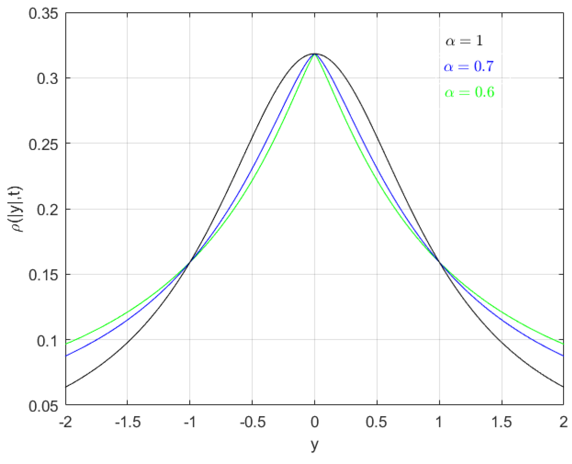
4. Hierarchy of Stable Distributions on Fractal Sets

In this section, we define stable distributions on thin Cantor-like sets and present examples such as fractal Cauchy and Gaussian stable distributions.

Definition of stable distributions. Let $X_1\left(t\right)$ and $X_2\left(t\right)$ be independent and identically distributed (iid) random variables on a thin Cantor-like set ($t\in C^{\beta }$) with mean $\mu \in (-\infty ,\infty )$ and variance $\sigma \in (0,\infty )$. A fractal random variable $X\left(t\right)$ with cumulative distribution function (CDF) $F_X\left(t\right)$ on the same fractal set is defined by [45]

$$X\left(t\right)=\frac{a_1{X}_1+a_2{X}_2-b}{a},$$

(32)

for constants $a,a_1,a_2\in (0,+\infty )$ and $b\in (-\infty ,+\infty )$. This X has the same CDF as $X_1$ and $X_2$, for given $a,b,a_1,a_2$, if the following condition holds

$$F_X\left(\frac{t}{a_1}\right)F_X\left(\frac{t}{a_2}\right)=F_X\left(\frac{t-b}{a}\right),t\in C^{\beta }.$$

(33)

In this case, $F_X\left(t\right)$ is called a ’stable’ fractal distribution function [46,47]. However, in general, the Equation (33) is difficult to solve for the function $F_X$, and so this is not a practical way to find stable fractal random variables. Therefore, we define the analogue of a characteristic function for a stable fractal random variable X as follows [46,47]

$${\mathsf{\Psi }}_X(\omega ;\lambda ,c,\nu ,\mu )=exp(i\mu S_F^{\alpha }\left(\omega \right)-\mathsf{\Phi }),$$

(34)

where the quantity $\mathsf{\Phi }$ is defined as

$$\mathsf{\Phi }=\left\{\begin{array}{cc}|c{S}_F^{\alpha }{\left(\omega \right)|}^{\lambda }(1-i\nu \mathrm{sgn}\left(S_F^{\alpha }\left(\omega \right)\right)tan\frac{\pi \lambda }{2}),\hfill & \lambda \ne 1;\hfill \\ |c{S}_F^{\alpha }{\left(\omega \right)|}^{\lambda }(1+i\nu \frac{2}{\pi }\mathrm{sgn}\left(S_F^{\alpha }\left(\omega \right)\right)log|S_F^{\alpha }\left(\omega \right)\left|\right),\hfill & \lambda =1.\hfill \end{array}\right.$$

(35)

where $i=\sqrt{-1}$, $\lambda \in (0,2]$ is a stability parameter, $\nu \in [-1,1]$ is a skewness parameter, $c\in (0,\infty )$ is a scale parameter, $\mu \in (-\infty ,+\infty )$ is a location parameter, and

$$\mathrm{sgn}\left(\omega \right)=\left\{\begin{array}{cc}1,\hfill & S_F^{\alpha }\left(\omega \right)>0;\hfill \\ 0,\hfill & S_F^{\alpha }\left(\omega \right)=0;\hfill \\ -1,\hfill & S_F^{\alpha }\left(\omega \right)<0.\hfill \end{array}\right.$$

(36)

In view of the upper bound $S_F^{\alpha }\left(\omega \right)\le {\omega }^{\alpha }$ we have

$${\mathsf{\Psi }}_X(\omega ;\lambda ,c,\nu ,\mu )\sim \left\{\begin{array}{cc}exp\left(i\mu {\omega }^{\alpha }-{\left|{\left(c\omega \right)}^{\alpha }\right|}^{\lambda }(1-i\nu \mathrm{sgn}\left({\omega }^{\alpha }\right)tan\frac{\pi \lambda }{2})\right),\hfill & \lambda \ne 1/\alpha ;\hfill \\ exp\left(i\mu {\omega }^{\alpha }{-|\left(c\omega \right)}^{\alpha }{|}^{\lambda }(1+i\nu (\frac{2}{\pi }\mathrm{sgn}\left({\omega }^{\alpha }\right)log|{\omega }^{\alpha }\left|\right)\right),\hfill & \lambda =1/\alpha .\hfill \end{array}\right.$$

(37)

If we choose $\mu =0$ and $\nu =0$, then we get the asymptotic behavior of Equation (37) as follows:

$${\mathsf{\Psi }}_X(\omega ;\lambda ,c,0,0)\sim exp\left[{-|\left(c\omega \right)}^{\alpha }{|}^{\lambda }\right],0<\lambda \le \frac{2}{\alpha }.$$

(38)

Here, if $\lambda <0$, then it would mean ${\mathsf{\Psi }}_X\left(\omega \right)=1$ as $\left|\omega \right|\to \infty$, and so there would be no fractal inverse Fourier transformation. In addition, $\lambda >\frac{2}{\alpha }$ would lead to the negative $f_X\left(t\right)$.

We consider some examples of fractal stable distributions.

• Gaussian stable distribution on fractal sets. In Equation (34) if we choose $\lambda =2$, $\nu =0$ and ${\sigma }^2=2c^2$, then we have

  $$\begin{array}{ccc}\hfill {\mathsf{\Psi }}_X(\omega ,2,c,0,\mu )& =& exp\left[i\mu S_F^{\alpha }\left(\omega \right)-\frac{1}{2}{\sigma }^2{\left|S_F^{\alpha }\left(\omega \right)\right|}^2\right].\hfill \end{array}$$

  (39)

  The asymptotic behavior of Equation (39) gives

  $$\begin{array}{c}\hfill {\mathsf{\Psi }}_X(\omega ,2,c,0,\mu )\sim exp\left[i\mu {\omega }^{\alpha }-\frac{1}{2}{\sigma }^2{\omega }^{2\alpha }\right],\end{array}$$

  (40)

  where $\sigma$ and $\mu$ are the variance and mean respectively. The corresponding probability distribution function, which is the inverse Fourier transformation of Equation (39), is as follows:

  $$\begin{array}{c}\hfill p(t,2,c,0,\mu )=\frac{1}{\sqrt{2\pi {\sigma }^2}}exp\left[\frac{{(t{\chi }_{C^{\beta }}-\mu )}^2}{2{\sigma }^2}\right].\end{array}$$

  (41)
• Cauchy stable distribution on fractal sets. If we choose $\lambda =1$, then Equation (34) gives

  $$\begin{array}{c}\hfill {\mathsf{\Psi }}_X(\omega ,1,1,0,\mu )=exp\left[i\mu S_F^{\alpha }\left(\omega \right)-\left|S_C^{\alpha }\left(\omega \right)\right|\right].\end{array}$$

  (42)

  The corresponding probability distribution function is

  $$\begin{array}{c}\hfill p(t,1,1,0,\mu )=\frac{1}{\pi {(t{\chi }_{C^{\beta }}-\mu )}^2+1)}.\end{array}$$

  (43)
• Levy $\alpha$-stable distribution on fractal sets. If we choose $\lambda =1/2$, then Equation (34) gives

  $$\begin{array}{ccc}\hfill {\mathsf{\Psi }}_X(\omega ,1/2,1,1,\mu )& =& exp\left[i\mu S_F^{\alpha }\left(\omega \right)-{\left|S_F^{\alpha }\left(\omega \right)\right|}^{1/2}(1-i\mathrm{sgn}{S}_F^{\alpha }\left(\omega \right))\right].\hfill \end{array}$$

  (44)

  In view of asymptotic behavior of Equation (44) one can write

  $$\begin{array}{c}\hfill {\mathsf{\Psi }}_X(\omega ,1/2,1,1,\mu )\sim exp\left[i\mu {\omega }^{\alpha }-{|\Gamma (1+\alpha ){\omega }^{\alpha }|}^{1/2}(1-isgn{\omega }^{\alpha })\right].\end{array}$$

  (45)

  The corresponding probability distribution function is

  $$\begin{array}{c}\hfill p(t,1/2,1,1,\mu )=\sqrt{\frac{1}{2\pi {(t{\chi }_{C^{\beta }}-\mu )}^3}}exp\left[\frac{-1}{2(t{\chi }_{C^{\beta }}-\mu )}\right].\end{array}$$

  (46)

Remark 1.

We can summarise the above results as follows.

1. 

If we choose $\lambda =2/\alpha$, in Equation (34) then the stable distribution has the mean and variance limited.

2. 

If we let $0<\lambda <1/\alpha$ in Equation (34), then the mean and variance are infinite.

3. 

If we substitute $1/\alpha <\lambda <2/\alpha$ into Equation (34), then the mean is finite and the variance is infinite (a heavy-tailed distribution).

Remark 2.

If X is a random variable on a fractal set, having stable distribution with exponent Equation (34) if we set $1/\alpha <\lambda <2/\alpha$, then $1/X^{\lambda }$ also has a stable distribution with exponent $1/\lambda$.

5. Physical Models for Fractal Stable Distributions

In this section, we suggest a physical model that can have a fractal stable distribution.

If we consider a random walk on a fractal thin Cantor-like set, then the fractal first passing time (FFPT), defined as the time when the walker hits a point $b\in C^{\beta }$, is a random variable. We suggest the following conditional probability distribution function [48] for the walker hitting b in the time interval $(t,t+dt)$:

$$p(t,b|0)=\frac{S_{C^{\beta }}^{\alpha }\left(b\right)}{\sqrt{4\pi D{t}^3}}exp\left[\frac{-S_{C^{\beta }}^{\alpha }{\left(b\right)}^2}{4Dt}\right],$$

(47)

where D is constant.

If we have two particles which have random walks on a fractal set with positions $X_1,X_2\in C^{\beta }$, then the new fractal random variable $Y=X_1/X_2$ has fractal Cauchy distribution. Here each $X_1,X_2$ has fractal Gaussian distribution.

To prove this, we suppose the probability distribution of Y is denoted $\rho (y,t)$ and work as follows

$$\begin{array}{cc}\hfill \rho (y,t)& ={\int }_{-\infty }^{\infty }{d}_F^{\alpha }{x}_1{\int }_{-\infty }^{\infty }{d}_F^{\alpha }{x}_2\frac{1}{4\pi Dt}exp\left[\frac{(-x_1^2-x_2^2){\chi }_{C^{\beta }}}{4Dt}\right]{\delta }_F^{\alpha }\left((y-\frac{x_1}{x_2}){\chi }_{C^{\beta }}\right)\hfill \\ & ={\int }_{-\infty }^{\infty }{d}_F^{\alpha }{x}_2\frac{|x_2{\chi }_{C^{\beta }}|}{4\pi Dt}exp\left[\frac{-x_2^2(1+y^2){\chi }_{C^{\beta }}}{4Dt}\right]\hfill \\ & =2{\int }_0^{\infty }{d}_F^{\alpha }{x}_2\frac{x_2{\chi }_{C^{\beta }}}{4\pi Dt}exp\left[\frac{-x_2^2(1+y^2){\chi }_{C^{\beta }}}{4Dt}\right]\hfill \\ & =\frac{1}{\pi (1+S_F^{\alpha }{\left(y\right)}^2)}.\hfill \end{array}$$

(48)

Then, the asymptotic behavior of Equation (48) is given by

$$\begin{array}{c}\hfill \rho (y,t)\sim \frac{1}{\pi (1+y^{2\alpha })}.\end{array}$$

(49)

In Figure 4 we have plotted $\rho \left(\right|y|,t)$ for the different values of $\alpha$.

Remark 3.

The red lines in the graphs above have shown the case with continuous support and $\alpha =1$. In this case, we recall standard results and the examples work out using conjugacy of fractal calculus and standard calculus.

6. Conclusions

In this paper, we have defined fractal random variables on fractal sets which are called thin Cantor-like sets. Fractal random variables with stable distribution have been given and corresponding models were discussed. Stable distributions on fractals give new conditions and orders related to the dimension of the set they have defined on them. The suggested random variables are not differentiable in the sense of ordinary calculus provided that they also appear in the reference list here.

References

1. Barnsley, M.F. Fractals Everywhere; Academic Press: Cambridge, MA, USA, 2014. [Google Scholar]
2. Mandelbrot, B.B. The Fractal Geometry of Nature; WH Freeman: New York, NY, USA, 1983; Volume 173. [Google Scholar]
3. Gazit, Y.; Berk, D.A.; Leunig, M.; Baxter, L.T.; Jain, R.K. Scale-invariant behavior and vascular network formation in normal and tumor tissue. Phys. Rev. Lett. 1995, 75, 2428–2431. [Google Scholar] [CrossRef] [PubMed]
4. Baish, J.W.; Jain, R.K. Fractals and cancer. Cancer Res. 2000, 60, 3683–3688. [Google Scholar] [PubMed]
5. Falconer, K. Techniques in Fractal Geometry; John Wiley and Sons: Hoboken, NJ, USA, 1997. [Google Scholar]
6. Balankin, A.S. Effective degrees of freedom of a random walk on a fractal. Phys. Rev. E 2015, 92, 062146. [Google Scholar] [CrossRef] [PubMed]
7. Zubair, M.; Mughal, M.J.; Naqvi, Q.A. Electromagnetic Fields and Waves in Fractional Dimensional Space; Springer: New York, NY, USA, 2012. [Google Scholar]
8. Czachor, M. Waves along fractal coastlines: From fractal arithmetic to wave equations. Acta Phys. Pol. B 2019, 50, 813–831. [Google Scholar] [CrossRef]
9. Chen, W.; Sun, H.-G.; Zhang, X.; Koroak, D. Anomalous diffusion modeling by fractal and fractional derivatives. Comput. Math. Appl. 2010, 59, 1754–1758. [Google Scholar] [CrossRef] [Green Version]
10. Sandev, T.; Iomin, A.; Kantz, H. Anomalous diffusion on a fractal mesh. Phys. Rev. E 2017, 95, 052107. [Google Scholar] [CrossRef] [PubMed]
11. Freiberg, U.; Zahle, M. Harmonic calculus on fractals-a measure geometric approach I. Potential Anal. 2002, 16, 265–277. [Google Scholar] [CrossRef]
12. Barlow, M.T.; Perkins, E.A. Brownian motion on the Sierpinski gasket. Probab. Theory Relat. Fields 1988, 79, 543–623. [Google Scholar] [CrossRef]
13. Kigami, J. Analysis on Fractals; Cambridge University Press: Cambridge, UK, 2001. [Google Scholar]
14. Uchaikin, V.V. Fractional Derivatives for Physicists and Engineers; Springer: Berlin, Germany, 2013; Volume 1. [Google Scholar]
15. Tatom, F.B. The relationship between fractional calculus and fractals. Fractals 1995, 3, 217–229. [Google Scholar] [CrossRef]
16. Nigmatullin, R.R.; Le Mehaute, A. Is there geometrical/physical meaning of the fractional integral with complex exponent? J. Non Cryst. Solids 2005, 351, 2888–2899. [Google Scholar] [CrossRef]
17. Cattani, C. Fractal and Fractional. Fractal Fract. 2017, 1, 1. [Google Scholar] [CrossRef]
18. Herrmann, R. Fractional Calculus: An Introduction for Physicists; World Scientific Publishing: Singapore, 2014. [Google Scholar]
19. Hilfer, R. Applications of Fractional Calculus in Physics; World Scientific Publishing Co.: Singapore, 2000. [Google Scholar]
20. Kolwankar, K.M.; Gangal, A.D. Fractional differentiability of nowhere differentiable functions and dimensions. Chaos 1996, 6, 505–513. [Google Scholar] [CrossRef] [PubMed] [Green Version]
21. Parvate, A.; Gangal, A.D. Calculus on fractal subsets of real-line I: Formulation. Fractals 2009, 17, 53–148. [Google Scholar] [CrossRef]
22. Parvate, A.; Gangal, A.D. Calculus on fractal subsets of real-line II: Conjugacy with ordinary calculus. Fractals 2011, 19, 271–290. [Google Scholar] [CrossRef]
23. Satin, S.; Parvate, A.; Gangal, A.D. Fokker–Planck equation on fractal curves. Chaos Solitons Fract. 2013, 52, 30–35. [Google Scholar] [CrossRef]
24. Parvate, A.; Satin, S.; Gangal, A.D. Calculus on fractal curves in Rn. Fractals 2011, 19, 15–27. [Google Scholar] [CrossRef]
25. Satin, S.; Gangal, A.D. Langevin Equation on Fractal Curves. Fractals 2016, 24, 1650028. [Google Scholar] [CrossRef]
26. Golmankhaneh, A.K.; Fernandez, A.; Golmankhaneh, A.K.; Baleanu, D. Diffusion on middle-ξ Cantor sets. Entropy 2018, 20, 504. [Google Scholar] [CrossRef]
27. Golmankhaneh, A.K.; Fernandez, A. Fractal Calculus of Functions on Cantor Tartan Spaces. Fractal Fract. 2018, 2, 30. [Google Scholar] [CrossRef]
28. Golmankhaneh, A.K.; Baleanu, D. Diffraction from fractal grating Cantor sets. J. Mod. Opt. 2016, 63, 1364–1369. [Google Scholar] [CrossRef]
29. Golmankhaneh, A.K. On the Fractal Langevin Equation. Fractal Fract. 2019, 3, 11. [Google Scholar] [CrossRef]
30. Golmankhaneh, A.K. Statistical Mechanics Involving Fractal Temperature. Fractal Fract. 2019, 3, 20. [Google Scholar] [CrossRef]
31. Jafari, F.K.; Asgari, M.S.; Pishkoo, A. The Fractal Calculus for Fractal Materials. Fractal Fract. 2019, 3, 8. [Google Scholar] [CrossRef]
32. Golmankhaneh, A.K. On the calculus of the parameterized fractal curves. Turk. J. Phys. 2017, 41, 418–425. [Google Scholar] [CrossRef]
33. Golmankhaneh, A.K. About Kepler’s Third Law on fractal-time spaces. Ain Shams Eng. J. 2018, 9, 2499–2502. [Google Scholar] [CrossRef]
34. Golmankhaneh, A.K.; Balankin, A.S. Sub-and super-diffusion on Cantor sets: Beyond the paradox. Phys. Lett. A 2018, 382, 960–967. [Google Scholar] [CrossRef]
35. Balankin, A.S.; Golmankhaneh, A.K.; Patiño-Ortiz, J.; Patiño-Ortiz, M. Noteworthy fractal features and transport properties of Cantor tartans. Phys. Lett. A 2018, 382, 1534–1539. [Google Scholar] [CrossRef]
36. Golmankhaneh, A.K.; Baleanu, D. Non-local Integrals and Derivatives on Fractal Sets with Applications. Open Phys. 2016, 14, 542–548. [Google Scholar] [CrossRef]
37. Shannon, C.E. A Mathematical Theory of Communication. Bell Syst. Tech. J. 1948, 27, 379–423. [Google Scholar] [CrossRef] [Green Version]
38. Kapur, J.N. Measures of Information and Their Applications; Wiley: New York, NY, USA, 1994. [Google Scholar]
39. Cattani, C. Fractional Calculus and Shannon Wavelet. Math. Probl. Eng. 2012, 2012, 26. [Google Scholar] [CrossRef]
40. Cattani, C.; Pierro, G. On the fractal geometry of DNA by the binary image analysis. Bull. Math. Biol. 2013, 75, 1544–1570. [Google Scholar] [CrossRef] [PubMed]
41. Heydari, M.H.; Hooshmandasl, M.R.; Ghaini, F.M.; Cattani, C. Wavelets method for solving fractional optimal control problems. Appl. Math. Comput. 2016, 286, 139–154. [Google Scholar] [CrossRef]
42. DiMartino, R.; Urbina, W. On Cantor-like sets and Cantor-Lebesgue singular functions. arXiv 2014, arXiv:1403.6554. [Google Scholar]
43. Cohen, S.N.; Elliott, R.J. Stochastic Calculus and Applications; Birkhäuser: New York, NY, USA, 2015; Volume 2. [Google Scholar]
44. Papoulis, A.; Pillai, S.U. Probability, Random Variables, and Stochastic Processes, 4th ed.; McGraw-Hill: New York, NY, USA, 2002. [Google Scholar]
45. Voit, J. The Statistical Mechanics of Financial Markets; Springer Science Business Media: Dodrecht, The Netherlands, 2005. [Google Scholar]
46. Breiman, L. Probability, Volume 7 of Classics in Applied Mathematics; Society for Industrial and Applied Mathematics (SIAM): Philadelphia, PA, USA, 1992. [Google Scholar]
47. Cizek, P.; Hardle, W.K.; Weron, R. Statistical Tools for Finance and Insurance; Springer Science Business Media: New York, NY, USA, 2005. [Google Scholar]
48. Khantha, M.; Balakrishnan, V. First passage time distributions for finite one-dimensional random walks. Pramana 1983, 21, 111–122. [Google Scholar] [CrossRef]
Figure 1. Figures for Section 2. (a) The thin Cantor-like set with β = 2 ; (b) staircase function corresponding to the thin Cantor-like set with β = 2 ; (c) the γ -dimension is α = 0 . 5 for the thin Cantor-like set with β = 2 ; (d) fractal characteristic function for the thin Cantor-like set with β = 2 .
Fractalfract 03 00031 g001
Figure 2. Figures for Example 1. (a) Probability density function of a fractal Cauchy random variable with α = 0.5, β = 2, a = 0.2; (b) distribution function of a fractal Cauchy random variable with α = 0.5, β = 2, a = 0.2; (c) characteristic function of a fractal Cauchy random variable with α = 0.5, β = 2, a = 0.2; (d) entropy of a fractal Cauchy random variable with a = 0.2.
Fractalfract 03 00031 g002
Figure 3. Figures for Example 2. (a) Probability density function of a fractal Laplace random variable with c = 1 , α = 0 . 5 , β = 2 , ν = 0 ; (b) distribution function of a fractal Laplace random variable with c = 1 , α = 0 . 5 , β = 2 , ν = 0 ; (c) characteristic function of a fractal Laplace random variable with c = 1 , α = 0 . 5 , β = 2 , ν = 0 ; (d) entropy of a fractal Laplace random variable with c = 1 .
Fractalfract 03 00031 g003
Figure 4. Graph of ρ ( | y | , t ) versus α .
Fractalfract 03 00031 g004