Partially Penetrated Well Solution of Fractal Single-Porosity Naturally Fractured Reservoirs

Abstract

In the oil industry, many reservoirs produce from partially penetrated wells, either to postpone the arrival of undesirable fluids or to avoid problems during drilling operations. The majority of these reservoirs are heterogeneous and anisotropic, such as naturally fractured reservoirs. The analysis of pressure-transient tests is a very useful method to dynamically characterize both the heterogeneity and anisotropy existing in the reservoir. In this paper, a new analytical solution for a partially penetrated well based on a fractal approach to capture the distribution and connectivity of the fracture network is presented. This solution represents the complexity of the flow lines better than the traditional Euclidean flow models for single-porosity fractured reservoirs, i.e., for a tight matrix. The proposed solution takes into consideration the variations in fracture density throughout the reservoir, which have a direct influence on the porosity, permeability, and the size distribution of the matrix blocks as a result of the fracturing process. This solution generalizes previous solutions to model the pressure-transient behavior of partially penetrated wells as proposed in the technical literature for the classical Euclidean formulation, which considers a uniform distribution of fractures that are fully connected. Several synthetic cases obtained with the proposed solution are shown to illustrate the influence of different variables, including fractal parameters.

1. Introduction

In the literature, several analytical solutions for modeling the behavior of pressure-transient tests of partially penetrated wells have been proposed [1,2,3,4,5,6,7,8,9,10]. Some of these works have proposed the use of point and line source solutions derived in the Laplace space, considering finite and infinite systems, with homogeneous and naturally fractured reservoirs [2,5,6,8,10]. Other studies considered gas anisotropic reservoirs using a uniform flow solution [9]. All of these works assumed reservoirs with Euclidean geometry, that is, they used traditional mass conservation and flow equations.

Starting from mass conservation and flow equations with fractal characteristics, the authors of [11,12,13,14] analyzed the behavior of the pressure-transient tests of single and double porosity reservoirs with fractal geometry. These studies established the existence of a power-law behavior during the transient period instead of the classical semi-logarithmic behavior that exists in reservoirs with Euclidean geometry. It has been demonstrated that the radial flow regime is a special case of more general fractal behavior. All these studies considered vertical fully penetrated wells. Up to date, no study has been presented that considers the pressure-transient behavior of partially penetrated wells produced from anisotropic heterogeneous reservoirs with fractal properties.

In this study, a single-porosity system was considered, which can be represented by a naturally fractured reservoir with a tight matrix, where the porosity and permeability of the system are due to the fracture network. Additionally, it was considered that there was a folding where the density of fractures was greater at the top of the anticline and decreased toward the flanks. Thus, there was a heterogeneous and anisotropic reservoir where the radial and vertical permeabilities were functions of the radial and vertical position, respectively. Due to the complexity of this fracture network, it was convenient to consider fractal geometry, instead of assuming a uniform distribution of fractures, and all fractures as being interconnected, as is considered in the traditional formulation with Euclidean geometry.

The purpose of this work was to obtain an analytical solution that represented the behavior of pressure-transient tests in vertical wells partially penetrating heterogeneous and anisotropic reservoirs with fractal geometry. The heterogeneity and anisotropy were due to a fracture network caused by the thrust of a salt dome.

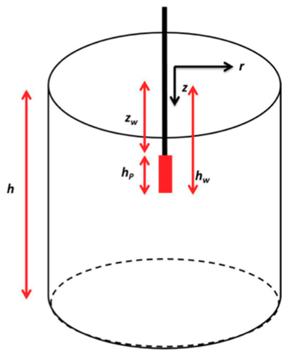
2. Problem Statement

The solution proposed in this study considered a closed cylindrical reservoir with a single porosity, i.e., a network of fractures may exist, but the matrix is compact and does not contribute to the reservoir response. The well was produced from a restricted interval of the formation. In the reservoir, there were fractal distributions of permeability and porosity in the radial and vertical directions, that is, it was a heterogeneous and anisotropic reservoir. Using the continuity equation in cylindrical coordinates:

$$\frac{1}{r}\frac{\partial }{\partial r}\left(r\rho v_r\right)+\frac{\partial }{\partial z}\left(\rho v_z\right)=-\frac{\partial \left(\rho \phi \right)}{\partial t},$$

(1)

considering a distribution of permeability in the fracture network like that existing in an anticline, where the radial permeability decreases as the radial distance from the center of the anticline increases, and the vertical permeability also decreases with the increment of vertical depth from the top of the anticline. Thus, the fractal distribution of permeability in the radial and vertical directions are given as follows:

$$k_r=k_{rw}{\left(\frac{r}{r_w}\right)}^{d_{fr}-{\theta }_r-D_r},$$

(2)

$$k_z=k_{zw}{\left(\frac{z}{r_w}\right)}^{d_{fz}-{\theta }_z-D_z},$$

(3)

where $k_{rw}$ and $k_{zw}$ represent the radial permeability at the center and the vertical permeability at the top of the anticline, respectively. D_r = 2 and D_z = 1 are the Euclidean dimensions in the horizontal and vertical directions, respectively. The fracture density is represented by the fractal dimensions $d_{fr}$ and $d_{fz}$, in the radial and vertical directions, respectively. ${\theta }_r$ and ${\theta }_z$ represent the connectivity indexes of the fracture network in the radial and vertical directions, respectively. The definition of radial permeability is similar to that used in References [11,12,13,14].

The porosity of the fracture network is also a function of the radial distance from the center of the anticline and the vertical position from the top of the anticline. Thus, using the fractal definition of porosity proposed by Cossio et al. [15] in 2D (r and z), the fracture porosity is given by:

$${\phi }_f=\frac{\overline{{\phi }_0}}{2}\left[{\left(\frac{r}{r_w}\right)}^{d_{fr}-D_r}+{\left(\frac{z}{r_w}\right)}^{d_{fz}-D_z}\right],$$

(4)

where ${\overline{\phi }}_0$ represents the average porosity in the near wellbore region at the top of the reservoir. In the following, we use ${\phi }_0={\overline{\phi }}_0/2$.

Assuming Darcy´s Law for the velocities in the radial and vertical directions and considering Equations (2)–(4) into Equation (1), the following equation can be obtained:

$$\frac{1}{r}\frac{\partial }{\partial r}\left(r\rho \frac{k_{rw}{(r/r_w)}^{d_{fr}-\theta r-Dr}}{\mu }\frac{\partial p}{\partial r}\right)+\frac{\partial }{\partial z}\left(\rho \frac{k_{zw}{(z/r_w)}^{d_{fz}-{\theta }_z-D_z}}{\mu }\frac{\partial p}{\partial z}\right)=\frac{\partial }{\partial t}\left(\rho {\phi }_0\left[{\left(\frac{r}{r_w}\right)}^{d_{fr}-D_r}+{\left(\frac{z}{r_w}\right)}^{d_{fz}-D_z}\right]\right).$$

(5)

It can be noted that instead of fractal derivatives, fractal definitions of the petrophysical properties are used in the derivation of this equation, following a similar path to that proposed in References [11,12,13,14,15,16,17]. Some applications of the use of fractional derivatives on the fluid flow in porous media are presented elsewhere [18,19,20,21]. Using the values of the Euclidean dimensions in the horizontal and vertical directions, D_r = 2 and D_z = 1, we obtained the following equation:

$$\frac{1}{r}\frac{\partial }{\partial r}\left(r\rho \frac{k_{rw}{(r/r_w)}^{d_{fr}-\theta r-2}}{\mu }\frac{\partial p}{\partial r}\right)+\frac{\partial }{\partial z}\left(\rho \frac{k_{zw}{(z/r_w)}^{d_{fz}-{\theta }_z-1}}{\mu }\frac{\partial p}{\partial z}\right)=\frac{\partial }{\partial t}\left(\rho {\phi }_0\left[{\left(\frac{r}{r_w}\right)}^{d_{fr}-2}+{\left(\frac{z}{r_w}\right)}^{d_{fz}-1}\right]\right).$$

(6)

Using the following definitions of dimensionless variables:

$$r_D=r/r_w.$$

(7)

$$z_D=z/h.$$

(8)

$$h_D=h/rw.$$

(9)

$$z_{wD}=z_w/h.$$

(10)

$$z_{wmD}=(z_w+h_p/2)/h.$$

(11)

$$h_{wD}=h_w/h.$$

(12)

$$h_{pD}=h_p/h.$$

(13)

$${\beta }_r=d_{fr}-{\theta }_r-1.$$

(14)

$${\beta }_z=d_{fz}-{\theta }_z-1.$$

(15)

$$\epsilon =k_{zw}/k_{rw}.$$

(16)

$$t_D=\frac{k_{rw}t}{{\phi }_0\mu c_t{r}_w^2}.$$

(17)

$$p_D=\frac{2\pi k_{rw}h\left(p_i-p\right)}{qB\mu }.$$

(18)

Considering a slightly compressible fluid of constant viscosity (µ), and small pressure gradients, we obtained:

$$\frac{1}{r_D}\frac{\partial }{\partial r_D}\left(r_D^{{\beta }_r}\frac{\partial p_D}{\partial r_D}\right)+\epsilon h_D^{{\beta }_z-2}\frac{\partial }{\partial z_D}\left(z_D{}^{{\beta }_z}\frac{\partial p_D}{\partial z_D}\right)=\left[r_D{}^{d_{fr}-2}+{\left(h_D{z}_D\right)}^{d_{fz}-1}\right]\frac{\partial p_D}{\partial t_D}.$$

(19)

In Figure 1, a diagram of the problem to be solved in cylindrical coordinates is shown.

Applying Newman’s method according to Razminia et al. [10], “the instantaneous Green function is equal to the product of the instantaneous Green functions in one and/or two directions”, in our case:

$$S(r_D,z_D,t_D)=S_r(r_D,t_D)\cdot S_z(z_D,t_D).$$

(20)

With the above, Equation (19) will be solved for the two directions independently.

3. Analytical Solution of the Problem

The solution was deduced by applying the methods of the Laplace’s transform, separation of variables, and Newman’s product using instantaneous source functions. In Appendix A, the procedure for obtaining the solution in the radial direction for total penetration, Equation (A7), can be found. This solution was used together with the solution in the vertical direction, Equation (A25), obtained in Appendix B, to acquire the solution for a partially penetrated well through the use of the Newman’s product. Thus, Equation (A33) is written as follows:

$${\overline{p}}_{wD}(s)=\frac{2}{h_{pD}^2\cdot s}\cdot {\displaystyle \sum _{n=0}^{\infty }\frac{K_{v_r}\left[{\psi }_n\right]{\left\{z_{wD}^{\frac{d_{fz}}{2}}{J}_{v_z-1}\left(a_n{z}_{wD}^{\frac{\left(2+{\theta }_z\right)}{2}}\right)-h_{wD}^{\frac{d_{fz}}{2}}{J}_{v_z-1}\left(a_n{h}_{wD}^{\frac{\left(2+{\theta }_z\right)}{2}}\right)\right\}}^2}{\left[\sqrt{s+{\lambda }_n}\left(\frac{1}{2}\right)\left[K_{v_r-1}\left[{\psi }_n\right]+K_{v_r+1}\left[{\psi }_n\right]\right]-\left(\frac{1-{\beta }_r}{2}\right)K_{v_r}\left[{\psi }_n\right]\right]a_n^2{\left[J_{v_z-1}^{}\left(a_n\right)-\frac{v_z}{a_n}{J}_{v_z}^{}\left(a_n\right)\right]}^2}},$$

(21)

where:

$${\psi }_n=\left(\frac{2}{2+{\theta }_r}\right)\sqrt{s+{\lambda }_n}.$$

(22)

If this expression is evaluated for $h_{pD}=1, z_{wD}=0,$ and $h_{wD}=1$, we obtain the fully-penetrated well solution:

$$\begin{array}{l}{\overline{p}}_{wD}(s)=\frac{K_{v_r}\left[\left(\frac{2}{2+{\theta }_r}\right)\sqrt{s}\right]}{s\left[\sqrt{s}\left(\frac{1}{2}\right)\left[K_{v_r-1}\left[\left(\frac{2}{2+{\theta }_r}\right)\sqrt{s}\right]+K_{v_r+1}\left[\left(\frac{2}{2+{\theta }_r}\right)\sqrt{s}\right]\right]-\left(\frac{1-{\beta }_r}{2}\right)K_{v_r}\left[\left(\frac{2}{2+{\theta }_r}\right)\sqrt{s}\right]\right]}\\ +\frac{2}{h_{pD}^2\cdot s}\cdot {\displaystyle \sum _{n=1}^{\infty }\frac{K_{v_r}\left[{\psi }_n\right]{\left\{z_{wD}^{\frac{d_{fz}}{2}}{J}_{v_z-1}\left(a_n{z}_{wD}^{\frac{\left(2+{\theta }_z\right)}{2}}\right)-h_{wD}^{\frac{d_{fz}}{2}}{J}_{v_z-1}\left(a_n{h}_{wD}^{\frac{\left(2+{\theta }_z\right)}{2}}\right)\right\}}^2}{\left[\sqrt{s+{\lambda }_n}\left(\frac{1}{2}\right)\left[K_{v_r-1}\left[{\psi }_n\right]+K_{v_r+1}\left[{\psi }_n\right]\right]-\left(\frac{1-{\beta }_r}{2}\right)K_{v_r}\left[{\psi }_n\right]\right]a_n^2{\left[J_{v_z-1}^{}\left(a_n\right)-\frac{v_z}{a_n}{J}_{v_z}^{}\left(a_n\right)\right]}^2}}\end{array}$$

(23)

where ${\lambda }_n$ are the characteristic values given by the roots of Equation (A17), and:

$$a_n=\frac{2}{2+{\theta }_z}\sqrt{\frac{{\lambda }_n{h}_D^{2+{\theta }_z}}{\epsilon }}.$$

(24)

The second term of Equation (23) represents the pseudo-skin due to partial penetration considering fractal behavior in both radial and vertical directions.

To include wellbore storage and mechanical skin effects, the following expression, given by Van Everdingen and Hurst [22], is applied:

$${\overline{p}}_{wD}\left(s\right)=\frac{s{\overline{p}}_D\left(s\right)+S}{s+C_D{s}^2\left[s{\overline{p}}_D\left(s\right)+S\right]}.$$

(25)

where ${\overline{p}}_D\left(s\right)$ is given by Equation (23).

4. Results

In this section, some results are presented with the proposed analytical solution given by Equations (23) and (25) in the case of wellbore storage and skin effects using Stehfest’s algorithm [23].

Figure 2, Figure 3, Figure 4 and Figure 5 show the solution for a Euclidean isotropic case (d_fr = 2.0, θ_r = 0, d_fz = 1.0, θ_z = 0), where the upper part of the formation is open to production. Figure 2 shows results without mechanical skin damage, $S=0$, where only the thickness of the formation varies. The dashed lines in Figure 2, Figure 3, Figure 4 and Figure 5 correspond to the pressure and pressure derivative given by Razminia et al. [10] for some Euclidian cases. In all cases, the agreement is excellent, so the proposed solution, Equation (23), is able to reproduce the Euclidian results as particular cases.

In Figure 3, the magnitude of the open interval varies, including the case of the fully penetrated well, keeping the thickness of the formation constant. In Figure 4 and Figure 5, the mechanical skin damage and wellbore storage vary, respectively, keeping the thickness of the formation and the open interval constant. All these cases are Euclidean and serve to evaluate the accuracy of the fractal analytic solution proposed for these cases.

The cases with fractal geometry are shown below. Figure 6 shows a case where the fractal dimension in the radial direction is varying, d_fr ≤ 2, where the value of 2 represents the Euclidean case (θ_r = 0). Thus, the traditional Euclidean case is a special case of the fractal case. In the Euclidean case, the classical spherical flow with a slope of −0.5, before the radial period, is present. It can be observed that this period of flow is not present for the fractal cases, where instead of the semi-logarithmic period, a power-law behavior can be observed in both the pressure drop and its derivative at late times during the transient period.

Figure 7 shows fractal cases where the connectivity index in the radial direction (θ_r) varies, and now all other parameters are kept constant, including the fractal dimension d_fr = 2. Again, the Euclidean case occurs when θ_r = 0, i.e., radial flow exists at late times during the transient period, and when θ_r > 0, the power-law response is present at these times.

In Figure 8 and Figure 9 the fractal dimension, d_fz, and the connectivity index, θ_z, are varied in the vertical direction, respectively, keeping the other parameters constant, including d_fr = 2, and θ_r = 0. The influence of d_fz and θ_z is observed only in the period before the radial flow. In these cases, when d_fz = 1.0 and θ_z = 0, the traditional Euclidean case is obtained again, with the presence of spherical flow before the radial period.

In Figure 10 and Figure 11, the influence of h_pD and the mechanical skin is shown, respectively, keeping the other parameters constant, including the fractal parameters. At large times within the transient period, the power-law behavior can be detected. In fact, in Figure 11, the presence of two power-law periods is observed.

Figure 12 and Figure 13 show the influence of the fractal parameters in the vertical direction, considering a fractal condition in the radial direction. In Figure 12, it is observed that the effect of the fractal dimension, d_fz, is not very strong; however, it can be expected that with the arrival of undesirable fluids to the producing well, this parameter could play an important role. In both figures, the presence of two power-law periods is observed. Figure 13 shows that when the connectivity of fractures or pores in the vertical direction decreases, or even becomes null (i.e., θ_z = 1), the late power-law period is delayed, which is an expected behavior.

Considering the above results, it can be deduced that the new proposed analytical solution may provide useful information for the proper development of a reservoir. However, it can be intuited that to determine all the parameters involved in the proposed analytical solution, it is necessary to use a robust optimizer, since a visual adjustment is expected to be very difficult to apply for a complex model such as the one proposed in this work.

5. Discussion

Taking into account the above results, and those presented by Posadas and Camacho [14], and the fact that there are many unknown parameters (S, C_D, $\epsilon$, $d_{fr}$, ${\theta }_r$, $d_{fz}$, ${\theta }_z$, k_r) to fully characterize this system, it is necessary to use robust optimization software in the type–curve matching process of both the pressure and its semi-logarithmic pressure derivative in order to obtain all of these parameters from well test data.

6. Conclusions

The novel analytical solution presented in this paper considers for the first time the application of fractal geometry to the problem of partial penetration. This is relevant because it allows the consideration of the variation of petrophysical properties with the scale or it takes into account the tortuosity of the flow lines in a cylindrical system. The solution was deduced by applying the methods of the Laplace’s transform, separation of variables, and Newman’s product using instantaneous source functions. Considering the results presented in this article, we can conclude the following:

• The new fractal analytical solution for a constant rate describes the pressure-transient behavior for partially penetrating wells in a single-porosity naturally fractured reservoir and includes the traditional Euclidean solution as a special case.
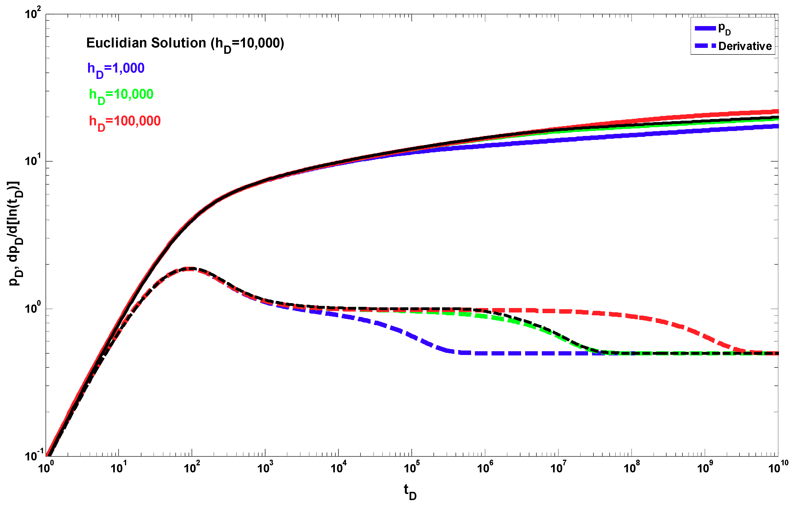
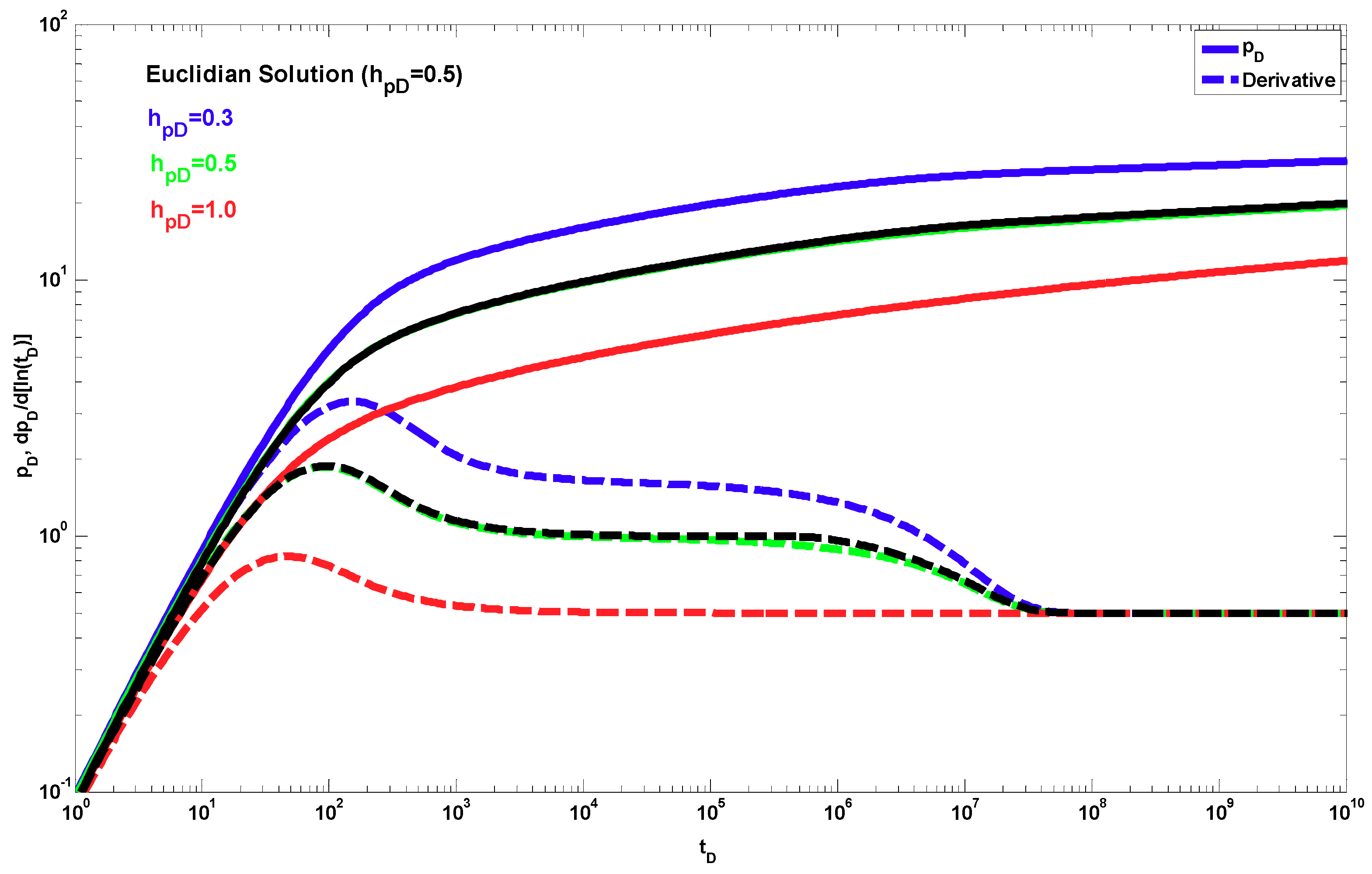
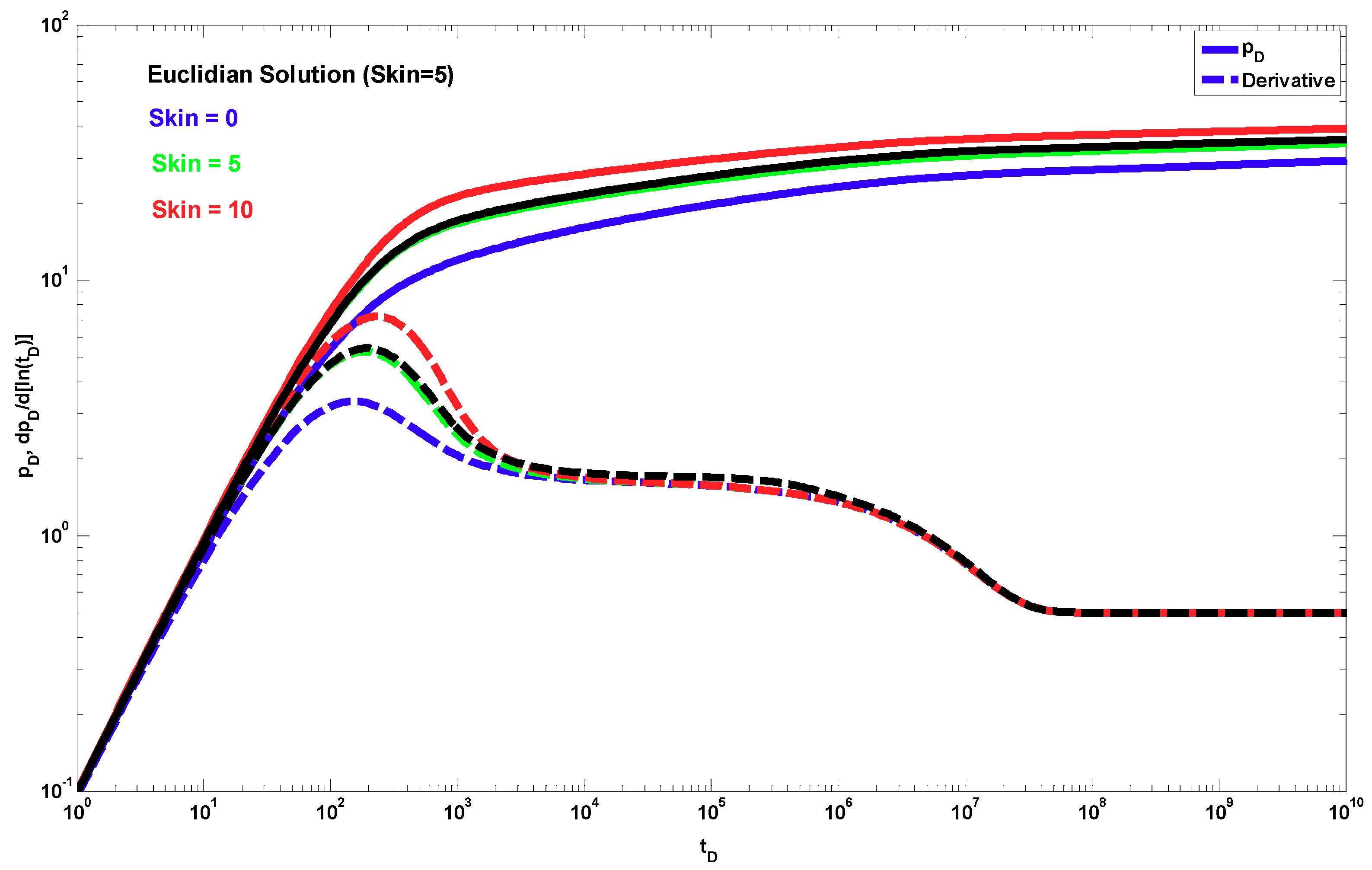
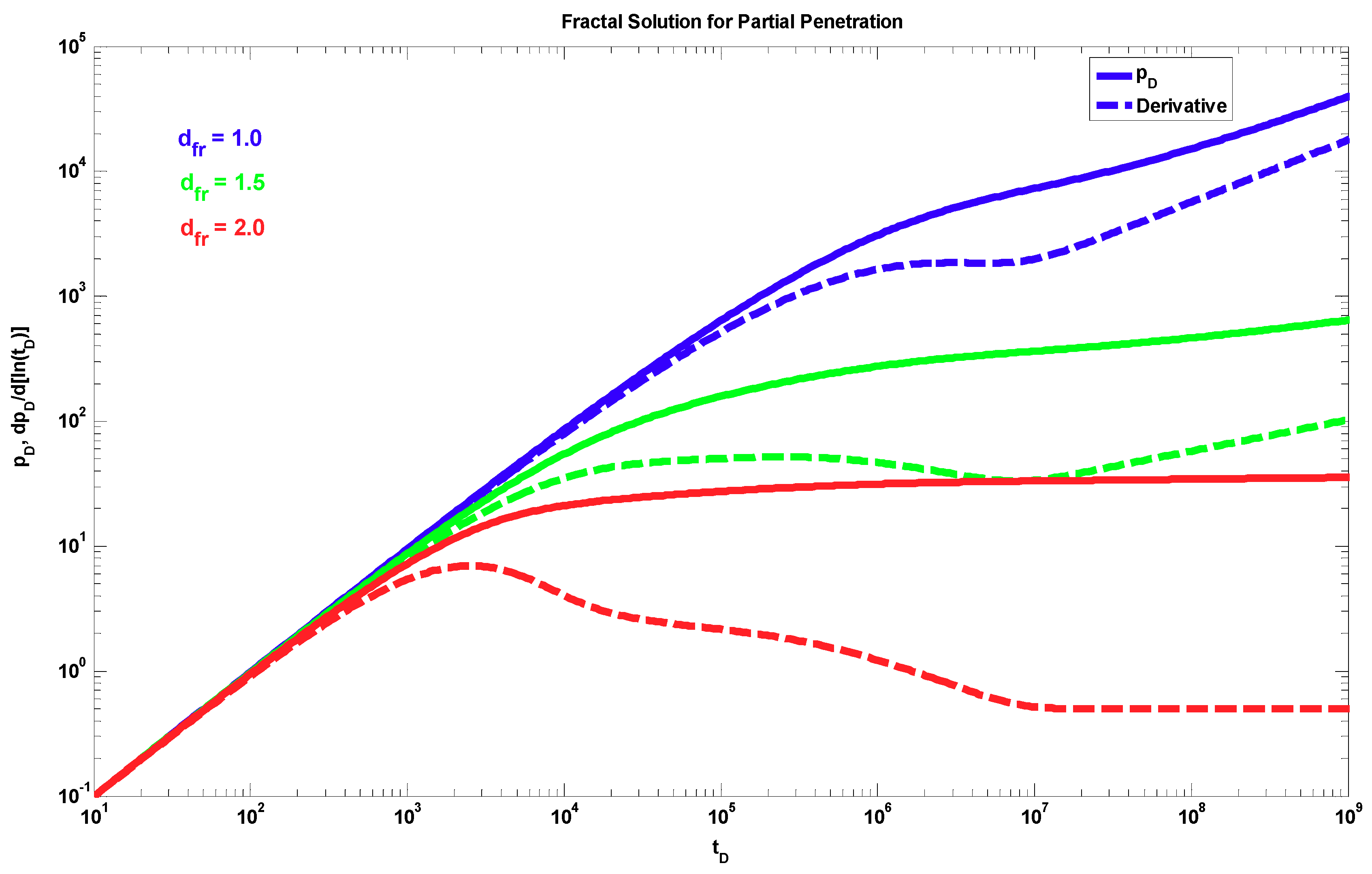
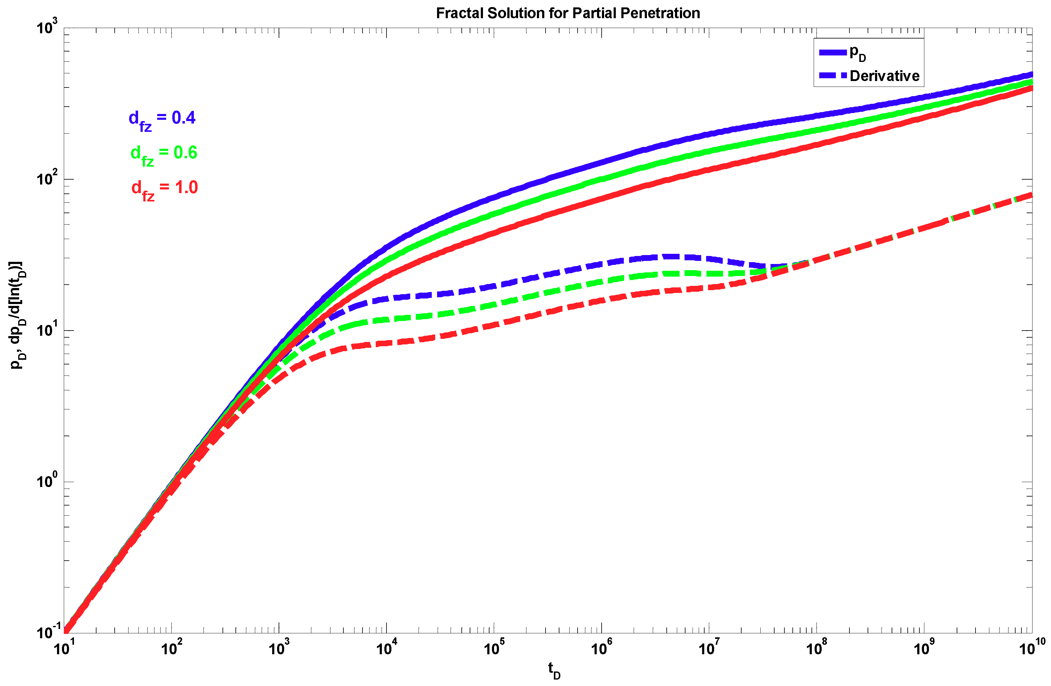
• The proposed fractal solution generates a power-law response at late times during the transient period after the wellbore storage, mechanical skin, and partial penetration effects have ended. This behavior occurs when the radial fractal parameters are different from the Euclidean values, i.e., d_fr < 2 and θ_r > 0.
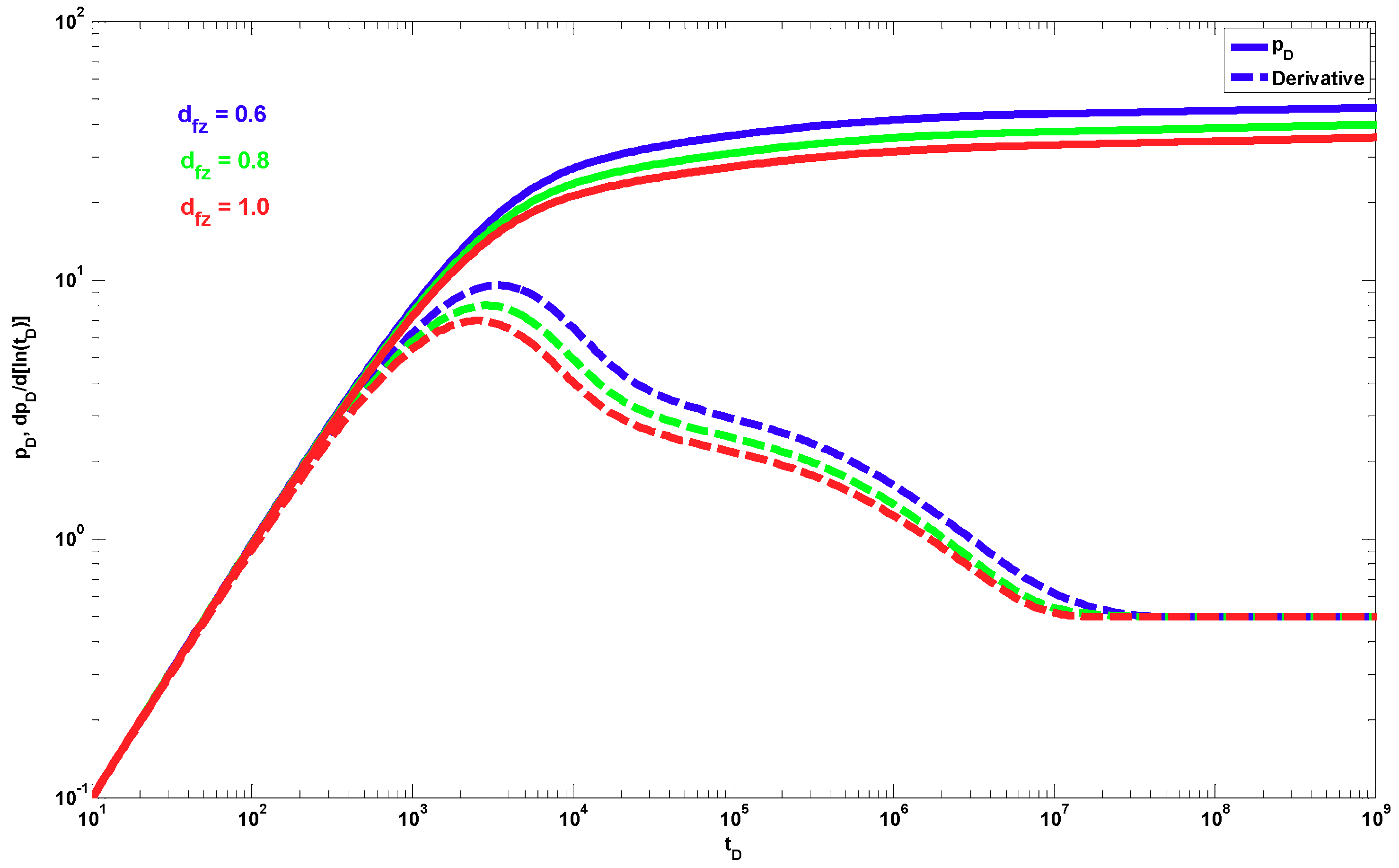
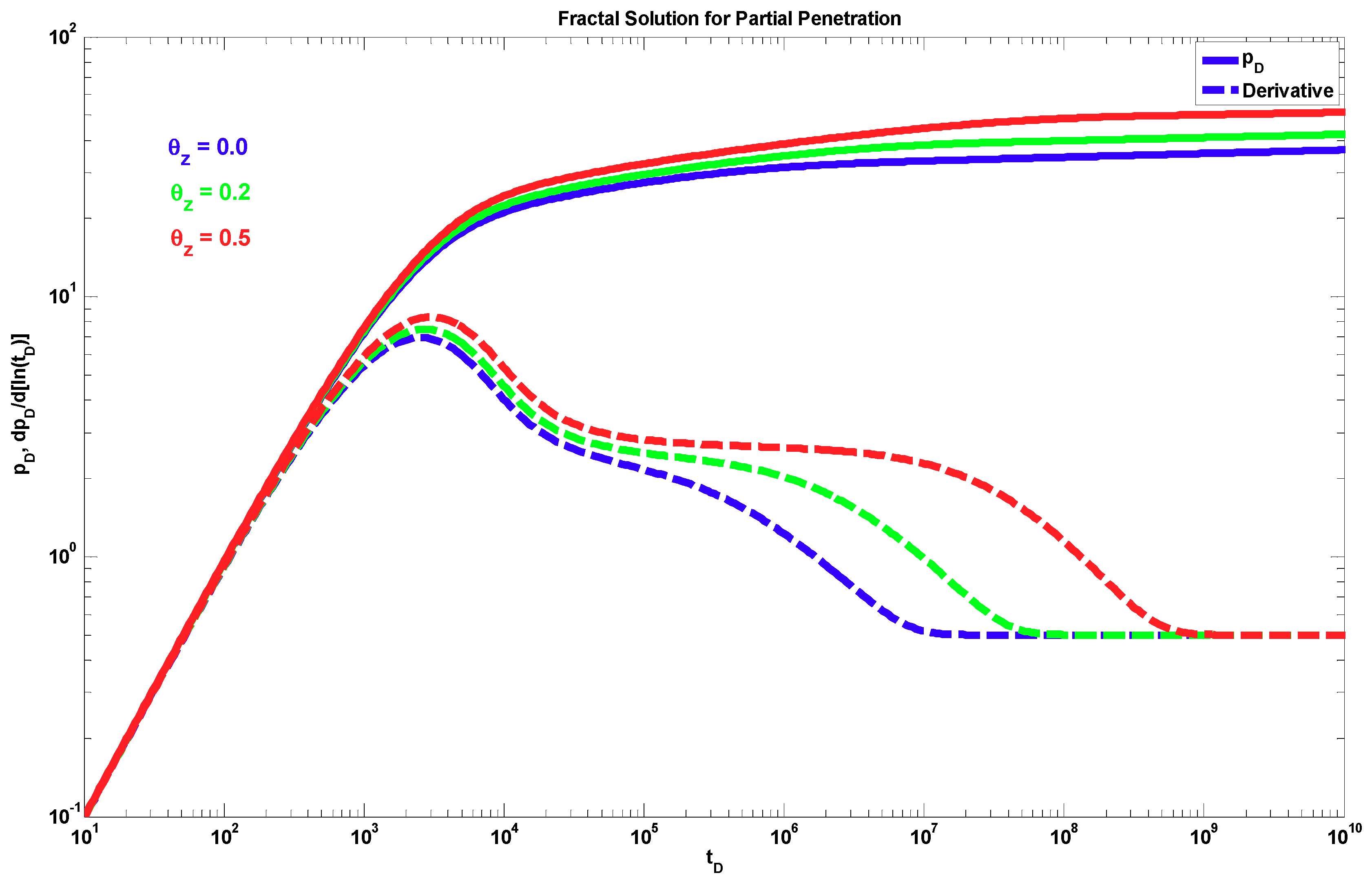
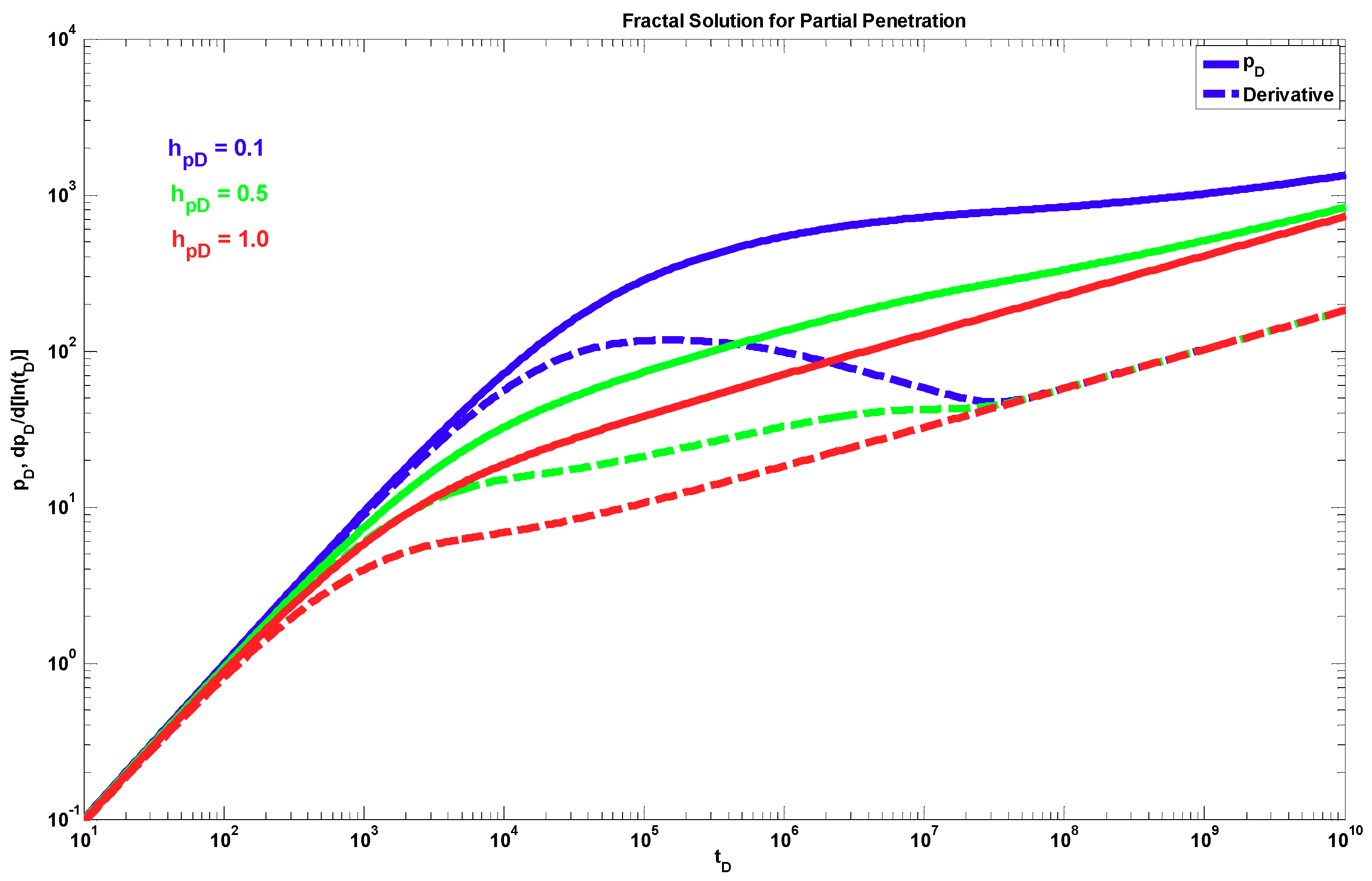
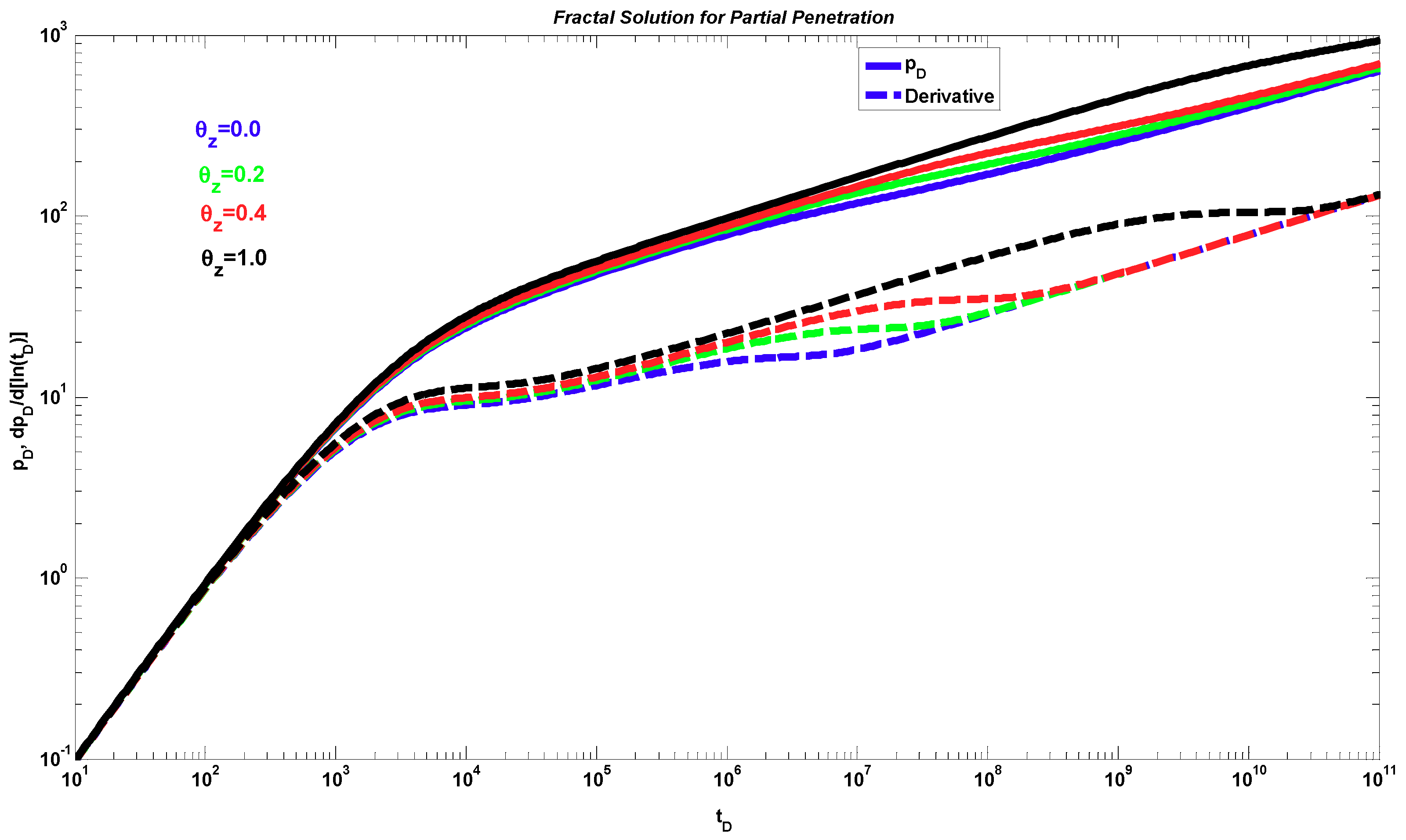
• A different behavior to the power-law response occurs when d_fz < 1 and θ_z > 0. The effect of these parameters is shown only during the partial penetration period, and after this period, the traditional radial behavior (if d_fr = 2 and θ_r = 0) or a power-law behavior (when d_fr < 2 and/or θ_r > 0) can be present.
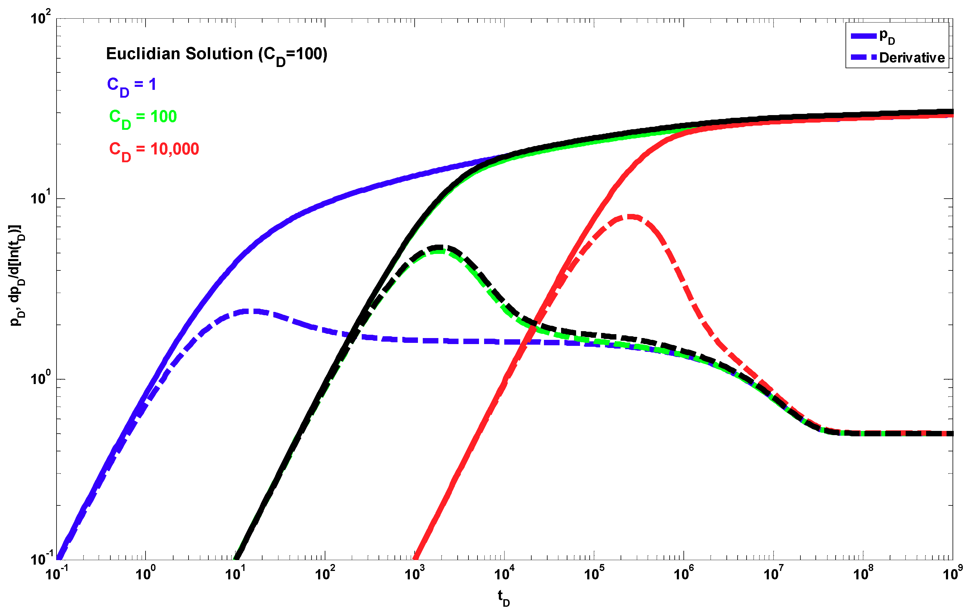
• The typical spherical flow regime due to partial penetration is only present when the fractal parameters in the radial direction have the Euclidean values, i.e., d_fr = 2 and θ_r = 0.
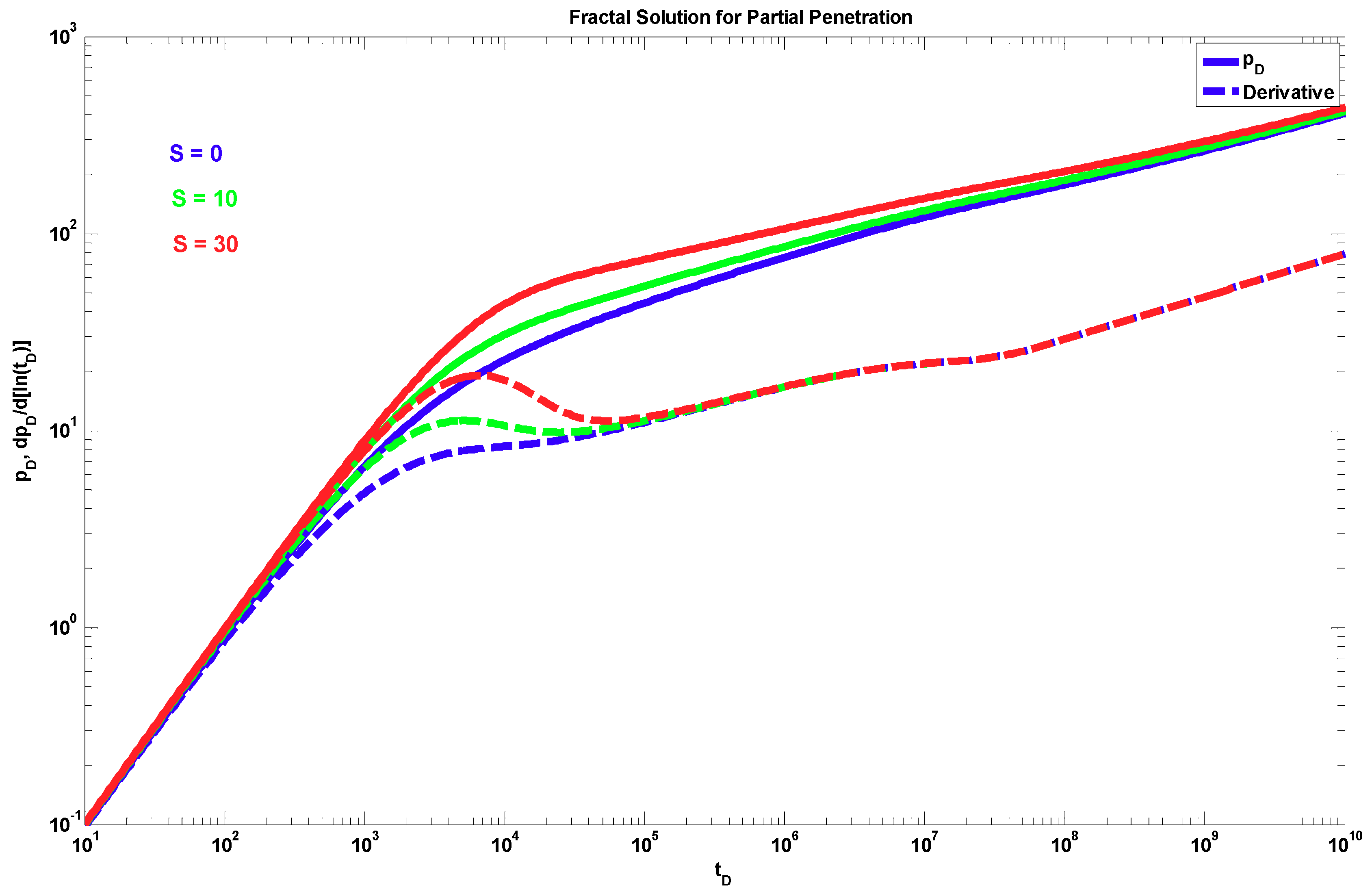
• An expression is provided to evaluate the pseudo-skin due to the partial penetration effects that consider fractal behavior in both the radial and vertical directions.
• To determine the pseudo-damage due to restricted penetration, horizontal permeability, vertical to horizontal permeability ratio, mechanical skin, and the four fractal parameters, it is necessary to resort to a type–curve matching process of the pressure data and its semi-logarithmic derivative using a robust optimizer that minimizes the difference between the real data and the analytical solution.

References

1. Brons, F.; Martin, V.E. The Effect of Restricted Fluid Entry on Well Productivity. In Proceedings of the 34th SPE Annual Meeting, Dallas, TX, USA, 4–7 October 1959. [Google Scholar]
2. Gringarten, A.C.; Ramey, H.J., Jr. An Approximate Infinite Conductivity Partially Penetrating Line-Source Solution Well. SPE J. 1975, 15, 140–148. [Google Scholar] [CrossRef]
3. Bilhartz, H.L., Jr.; Ramey, H., Jr. The Combined Effect of Storage, Skin, and Partial Penetration on Well Test Analysis. In Proceedings of the SPE 52nd Annual Fall Technical Conference and Exhibition, Denver, CO, USA, 19–21 October 1977. [Google Scholar]
4. Yildiz, T.; Bassiouni, Z. Transient Pressure Analysis in Partially-Penetrating Wells. In Proceedings of the SPE International Technical Meeting, Calgary, AB, Canada, 10–13 June 1990. [Google Scholar]
5. Ozkan, E.; Raghavan, R. New Solutions for Well-Test-Analysis Problems: Part 1—Analytical Considerations. SPE Form. Eval. 1991, 6, 359–368. [Google Scholar] [CrossRef]
6. Ozkan, E.; Raghavan, R. New Solutions for Well-Test-Analysis Problems: Part 2—Computational Considerations and Applications. SPE Form. Eval. 1991, 6, 369–378. [Google Scholar] [CrossRef]
7. Bui, T.D.; Mamora, D.D.; Lee, W.J. Transient Pressure Analysis for Partially Penetrating Wells in Naturally Fractured Reservoirs. In Proceedings of the SPE Rocky Mountain Regional/Low Permeability Reservoirs Symposium and Exhibition, Denver, CO, USA, 12–15 March 2000. [Google Scholar]
8. Fuentes, G.; Camacho, R.; Vasquez, M. Pressure Transient and Decline Curve Behaviors for Partially Penetrating Wells Completed in Naturally Fractured-Vuggy Reservoirs. In Proceedings of the 2004 SPE International Petroleum Conference in Mexico, Puebla Pue, 7–9 November 2004. [Google Scholar]
9. Miranda, F.; Barreto, A.; Peres, A. A Novel Uniform-Flux Solution based on Green’s Functions for Modeling the Pressure Transient Behavior of a Restricted-Entry Well in Anisotropic Gas Reservoirs. SPE J. 2016, 21, 1–870. [Google Scholar] [CrossRef]
10. Razminia, K.; Razminia, A.; Dastikhan, Z. A comprehensive Solution for Partially Penetrating Wells with Various Reservoir Structures. J. Oil Gas Petrochem. Tech. 2016, 3, 1. [Google Scholar]
11. Chang, J.; Yortsos, Y.C. Pressure Transient Analysis of Fractal Reservoirs. SPE Form. Eval. 1990, 289, 31. [Google Scholar] [CrossRef]
12. Acuña, J.A.; Ershaghi, I.; Yortsos, Y.C. Practical Application of Fractal Pressure-Transient Analysis in Naturally Fractured Reservoirs. SPE Form. Eval. 1995, 10, 173–179. [Google Scholar] [CrossRef]
13. Flamenco, L.F.; Camacho, R.G. Determination of Fractal Parameters of Fractured Networks Using Pressure-Transient Data. SPE Reserv. Eval. Eng. 2003, 6, 1. [Google Scholar]
14. Posadas, R.; Camacho, R.G. Influence and determination of Mechanical Skin in a Reservoir with a Fractal Behavior. In Proceedings of the SPE Heavy and Extra Heavy Oil Conference, Lima, Peru, 19–20 October 2016. [Google Scholar]
15. Cossio, M.; Moridis, G.J.; Blasingame, T.A. A Semianalytic Solution for Flow in Finite-Conductivity Vertical Fractures by Use of Fractal Theory. SPE J. 2013, 18, 83–96. [Google Scholar] [CrossRef]
16. Wang, W.; Shahvali, M.; Su, Y. A semi-analytical fractal model for production from tight oil reservoirs with hydraulically fractured horizontal wells. Fuel 2015, 158, 612–618. [Google Scholar] [CrossRef]
17. Wei, Y.; He, D.; Wang, J.; Qi, Y. A Coupled Model for Fractured Shale Reservoirs with Characteristics of Continuum Media and Fractal Geometry. In Proceedings of the SPE Asia Pacific Unconventional Resources Conference and Exhibition, Brisbane, Australia, 9–11 November 2015. [Google Scholar]
18. Raghavan, R.; Chen, C. Rate decline, power laws, and subdiffusion in fractured rocks. In Proceedings of the SPE Low Perm Symposium, Denver, CO, USA, 5–6 May 2016. [Google Scholar]
19. Fan, W.; Jiang, X.; Chen, S. Parameter estimation for the fractional fractal diffusion model based on its numerical solution. Comput. Math. Appl. 2016, 71, 642–651. [Google Scholar] [CrossRef]
20. Xu, Y.; He, Z.; Agrawal, O.P. Numerical and analytical solutions of new generalized fractional diffusion equation. Comput. Math. Appl. 2013, 66, 2019–2029. [Google Scholar] [CrossRef]
21. Raghavan, R.; Chen, C. Fractional diffusion in rocks produced by horizontal wells with multiple, transverse hydraulic fractures of finite conductivity. J. Pet. Sci. Eng. 2013, 109, 133–143. [Google Scholar] [CrossRef]
22. Van Everdingen, A.F.; Hurst, W. The Application of Laplace Transformation to Flow Problems in Reservoirs. Trans. AIME 1949, 180, 305–324. [Google Scholar] [CrossRef]
23. Stehfest, H. Numerical Inversion of Laplace Transforms. Commun. ACM 1970, 13, 47. [Google Scholar] [CrossRef]
24. Lebedev, N.N. Special Functions and Their Applications; Prentice-Hall: Upper Saddle River, NJ, USA, 1965. [Google Scholar]
25. Bramowitz, M.; Stegun, I. Handbook of Mathematical Functions; Dover Publications: New York, NY, USA, 1965. [Google Scholar]
26. Gradshteyn, I.S.; Ryzhik, I.M. Table of Integrals, Series, and Products; Academic Press: Cambridge, MA, USA, 2007. [Google Scholar]
Figure 1. Problem in cylindrical coordinates.
Fractalfract 03 00023 g001
Figure 2. Euclidean case: z w D = 0 , h p D = 0.5 , S = 0 , C D = 10 , ε = 1 , d f r = 2 , θ r = 0 , d f z = 1 , θ z = 0 .
Fractalfract 03 00023 g002
Figure 3. Euclidean case: z w D = 0 , h D = 10 , 000 , S = 0 , C D = 10 , ε = 1 , d f r = 2 , θ r = 0 , d f z = 1 , θ z = 0 .
Fractalfract 03 00023 g003
Figure 4. Euclidean case: z w D = 0 , h D = 10 , 000 , h p D = 0.3 , C D = 10 , ε = 1 , d f r = 2 , θ r = 0 , d f z = 1 , θ z = 0 .
Fractalfract 03 00023 g004
Figure 5. Euclidean case: z w D = 0 , h D = 10 , 000 , h p D = 0.3 , S = 1 , ε = 1 , d f r = 2 , θ r = 0 , d f z = 1 , θ z = 0 .
Fractalfract 03 00023 g005
Figure 6. Fractal case: z w D = 0.4 , h D = 10,000 , h p D = 0.2 , S = 0 , C D = 100 , ε = 1 , d f z = 1 , θ z = 0 .
Fractalfract 03 00023 g006
Figure 7. Fractal case: z w D = 0.4 , h D = 10,000 , h p D = 0.2 , S = 0 , C D = 100 , ε = 1 , d f r = 2 , d f z = 1 , θ z = 0 .
Fractalfract 03 00023 g007
Figure 8. Fractal case: z w D = 0.4 , h D = 10 , 000 , h p D = 0.2 , S = 0 , C D = 100 , ε = 1 , d f r = 2.0 , θ r = 0 , θ z = 0 .
Fractalfract 03 00023 g008
Figure 9. Fractal case: z w D = 0.4 , h D = 10 , 000 , h p D = 0.2 , S = 0 , C D = 100 , ε = 1 , d f r = 2.0 , θ r = 0 , d f z = 1.0 .
Fractalfract 03 00023 g009
Figure 10. Fractal case: z w D = 0 , h D = 10 , 000 , S = 0 , C D = 100 , ε = 1 , d f r = 1.5 , θ r = 0 , d f z = 1.0 , θ z = 0 .
Fractalfract 03 00023 g010
Figure 11. Fractal case: z w D = 0.2 , h p D = 0.6 , h D = 10 , 000 , C D = 100 , ε = 1 , d f r = 1.8 , θ r = 0.3 , d f z = 1.0 , θ z = 0.2 .
Fractalfract 03 00023 g011
Figure 12. Fractal case: z w D = 0.2 , h p D = 0.6 , h D = 10 , 000 , S = 0 , C D = 100 , ε = 1 , d f r = 1.8 , θ r = 0.3 , θ z = 0.1 .
Fractalfract 03 00023 g012
Figure 13. Fractal case: z w D = 0.2 , h p D = 0.6 , h D = 10 , 000 , S = 0 , C D = 100 , ε = 1 , d f r = 1.8 , θ r = 0.3 , d f z = 0.8 .
Fractalfract 03 00023 g013