Poiseuille Flow of a Non-Local Non-Newtonian Fluid with Wall Slip: A First Step in Modeling Cerebral Microaneurysms

Abstract
:1. Introduction
- (1)
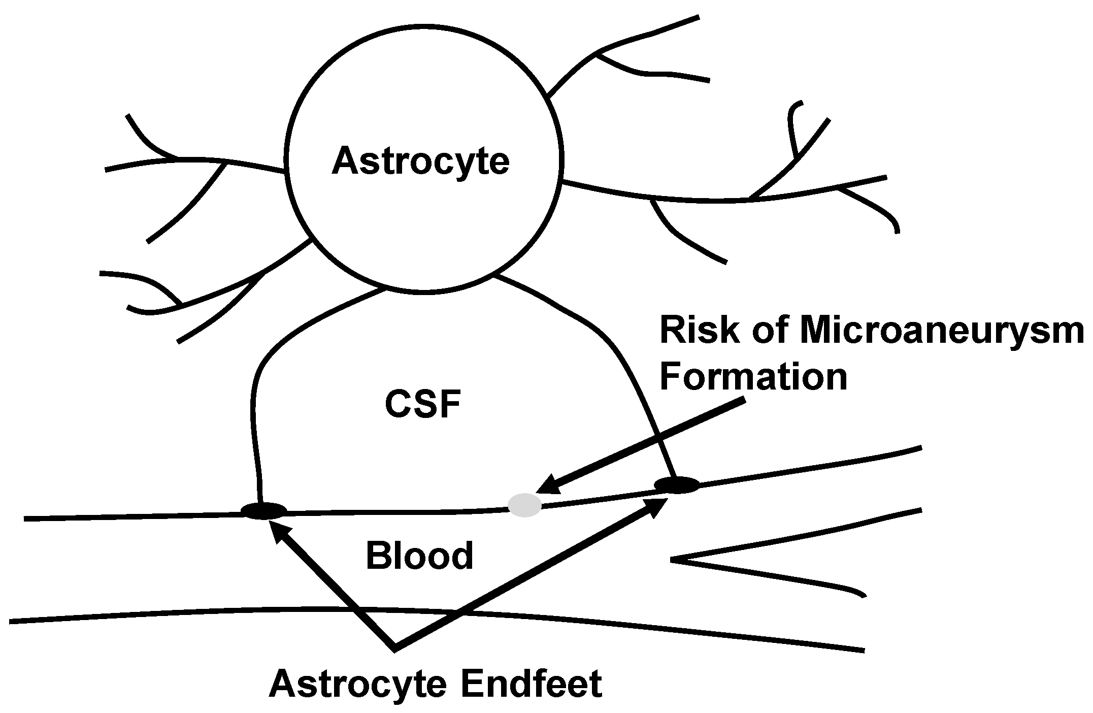
- a mechanism for the formation, growth and rupture of microaneurysms that involve the coupled dynamics of blood, arterioles and neuroglia was proposed,
- (2)
- a non-local constitutive law involving spatial fractional order Caputo derivatives and only two physical parameters ( and ) was proposed to describe the non-Newtonian behavior of blood,
- (3)
- a non-local slip condition at the blood-vascular wall interface was introduced,
- (4)
- analytic solutions to a Poiseuille flow through an axi-symmetric circular rigid and impermeable pipe with wall slip were proposed and
- (5)
- numerical simulations indicated that hypertension might contribute to the formation of microaneurysms, which agrees with some clinical studies.
2. Mathematical Model
2.1. Non-Local Kinematics
- if and is in :
- if
- if :
2.2. Poiseuille Flow
2.3. Two Slip Conditions
2.4. Non-Dimensionalization
3. Results
4. Conclusions
Conflicts of Interest
References
- Liebeskind, D.S. Cerebral Aneurysms: Practice Essentials, Background, Pathophysiology. Available online: http://emedicine.medscape.com/article/1161518-overview (accessed on 7 October 2017).
- Newman, E.A. Glial cell regulation of neuronal activity and blood flow in the retina by release of gliotransmitters. Philos. Trans. R. Soc. B 2015, 370. [Google Scholar] [CrossRef] [PubMed]
- Aguilar, E.; Friedlander, M.; Gariano, R.F. Endothelial proliferation in diabetic retinal microaneurysms. Arch. Ophthalmol. 2003, 121, 740–741. [Google Scholar] [CrossRef] [PubMed]
- Rosenblum, W.I. Miliary aneurysms and “fibrinoid” degeneration of cerebral blood vessels. Hum. Pathol. 1977, 8, 133–139. [Google Scholar] [CrossRef]
- Rosenblum, W.I. Fibrinoid necrosis of small brain arteries and arterioles and miliary aneurysms as causes of hypertensive hemorrhage: A critical reappraisal. Acta Neuropathol. 2008, 116, 361–369. [Google Scholar] [CrossRef] [PubMed]
- Hussain, S.; Barbarite, E.; Chaudhry, N.S.; Gupta, K.; Dellarole, A.; Peterson, E.C.; Elhammady, M.S. Search for biomarkers of intracranial aneurysms: A systematic review. World Neurosurg. 2015, 84, 1473–1483. [Google Scholar] [CrossRef] [PubMed]
- Liang, E.I.; Makino, H.; Tada, Y.; Wada, K.; Hashimoto, T. Animal models of intracranial aneurysms. In Translational Stroke Research from Target Selection to Clinical Trials; Lapchak, P.A., Zhang, J.H., Eds.; Springer: New York, NY, USA, 2012; pp. 585–593. ISBN 978-1-4419-9530-8. [Google Scholar]
- Cebral, J.R.; Castro, M.A.; Appanaboyina, S.; Putman, C.M.; Millan, D.; Frangi, A.F. Efficient pipeline for image-based patient-specific analysis of cerebral aneurysm hemodynamics: Technique and sensitivity. IEEE Trans. Med. Imaging 2005, 24, 457–467. [Google Scholar] [CrossRef] [PubMed]
- Kulcsár, Z.; Ugron, Á.; Marosfői, M.; Berentei, Z.; Paál, G.; Szikora, I. Hemodynamics of cerebral aneurysm initiation: The role of wall shear stress and spatial wall shear stress gradient. AJNR Am. J. Neuroradiol. 2011, 32, 587–594. [Google Scholar] [CrossRef] [PubMed]
- Jou, L.-D.; Lee, D.H.; Morsi, H.; Mawad, M.E. Wall shear stress on ruptured and unruptured intracranial aneurysms at the internal carotid artery. AJNR Am. J. Neuroradiol. 2008, 29, 1761–1767. [Google Scholar] [CrossRef] [PubMed]
- Meng, H.; Tutino, V.M.; Xiang, J.; Siddiqui, A. High WSS and low WSS? Complex interactions of hemodynamics with intracranial aneurysm initiation, growth, and rupture: Toward a unifying hypothesis. AJNR Am. J. Neuroradiol. 2014, 35, 1254–1262. [Google Scholar] [CrossRef] [PubMed]
- Oubel, E.; DeCraene, M.; Putman, C.M.; Cebral, J.R.; Frangi, A.F. Analysis of intracranial aneurysm wall motion and its effects on hemodynamic patterns. Proc. SPIE Med. Imaging 2007, 6511. [Google Scholar] [CrossRef]
- Xu, B.-N.; Wang, F.-Y.; Liu, L.; Zhang, X.-J.; Ju, H.-Y. Hemodynamics model of fluid-solid interaction in internal carotid artery aneurysms. Neurosurg. Rev. 2011, 34, 39–47. [Google Scholar] [CrossRef]
- Ngoepe, M.N.; Ventikos, Y. Computational modelling of clot development in patient-specific cerebral aneurysm cases. J. Thromb. Haemost. 2016, 14, 262–272. [Google Scholar] [CrossRef] [PubMed]
- Grinberg, L.; Fedosov, D.A.; Karniadakis, G.E. Parallel multiscale simulations of a brain aneurysm. J. Comp. Phys. 2013, 244, 131–147. [Google Scholar] [CrossRef] [PubMed]
- Paudel, P.; Rohlf, K. Flow with slip through an aneurysm using particle-based methods. In Proceedings of the 23rd Canadian Congress of Applied Mechanics (CANCAM), Vancouver, BC, Canada, 5–9 June 2011; pp. 1015–1019. [Google Scholar]
- Hodis, S.; Zamir, M. Arterial wall tethering as a distant boundary condition. Phys. Rev. E 2009, 80, 051913. [Google Scholar] [CrossRef] [PubMed]
- Hodis, S.; Zamir, M. Pulse wave velocity as a diagnostic index: The pitfalls of tethering versus stiffening of the arterial wall. J. Biomech. 2011, 44, 1367–1373. [Google Scholar] [CrossRef] [PubMed]
- Bhavsar, A.R.; Emerson, G.G.; Emerson, M.V.; Browning, D.J. Diabetic retinopathy. In Diabetic Retinopathy Evidence-Based Management; Browning, D.J., Ed.; Springer: New York, NY, USA, 2010; pp. 53–75. [Google Scholar]
- Zamir, M. Hemo-Dynamics; Springer: New York, NY, USA, 2016. [Google Scholar]
- Fisher, D.J.; Torrence, N.J.; Sprung, R.J.; Spence, D.M. Determination of erythrocyte deformability and its correlation to cellular ATP release using microbore tubing with diameters that approximate resistance vessels in vivo. Analyst 2003, 128, 1163–1168. [Google Scholar] [CrossRef]
- Metea, M.R.; Newman, E.A. Glial cells dilate and constrict blood vessels: a mechanism of neurovascular coupling. J. Neurosci. 2006, 26, 2862–2870. [Google Scholar] [CrossRef] [PubMed]
- Gordon, G.R.J.; Mulligan, S.J.; MacVicar, B.A. Astrocyte control of the cerebrovasculature. Glia 2007, 55, 1214–1221. [Google Scholar] [CrossRef] [PubMed]
- Petzold, G.C.; Murthy, V.N. Role of astrocytes in neurovascular coupling. Neuron 2011, 71, 782–797. [Google Scholar] [CrossRef] [PubMed]
- MacVicar, B.A.; Newman, E.A. Astrocyte regulation of blood flow in the brain. Cold Spring Harb. Perspect. Biol. 2015, 7, a020388. [Google Scholar] [CrossRef] [PubMed]
- Iadecola, C.; Nedergaard, M. Glial regulation of the cerebral microvasculature. Nat. Neurosci. 2007, 10, 1369–1376. [Google Scholar] [CrossRef] [PubMed]
- Fung, Y.C. Biomechanics: Mechanical Properties of Living Tissues; Springer: New York, NY, USA, 1993. [Google Scholar] [CrossRef]
- Tomaiuolo, G.; Lanotte, L.; D’Apolito, R.; Cassinese, A.; Guido, S. Microconfined flow behavior of red blood cells. Med. Eng. Phys. 2016, 38, 11–16. [Google Scholar] [CrossRef] [PubMed]
- Monson, K.L.; Goldsmith, W.; Barbaro, N.M.; Manley, G.T. Axial mechanical properties of fresh human cerebral blood vessels. J. Biomech. Eng. 2003, 125, 288–294. [Google Scholar] [CrossRef] [PubMed]
- Drapaca, C.S.; Sivaloganathan, S. A fractional model of continuum mechanics. J. Elast. 2012, 107, 105–123. [Google Scholar] [CrossRef]
- Santisakultarm, T.P.; Cornelius, N.R.; Nishimura, N.; Schafer, A.I.; Silver, R.T.; Doerschuk, P.C.; Olbricht, W.L.; Schaffer, C.B. In vivo two-photon excited fluorescence microscopy reveals cardiac- and respiration-dependent pulsatile blood flow in cortical blood vessels in mice. Am. J. Physiol. Heart Circ. Physiol. 2012, 302, H1367–H1377. [Google Scholar] [CrossRef] [PubMed]
- Zhong, Z.; Song, H.; Chui, T.Y.P.; Petrig, B.L.; Burns, S. Noninvasive measurements and analysis of blood velocity profiles in human retinal vessels. Investig. Ophthalmol. Vis. Sci. 2011, 52, 4151–4157. [Google Scholar] [CrossRef] [PubMed]
- West, B.J. Fractional Calculus View of Complexity: Tomorrow’s Science; CRC Press: Boca Raton, FL, USA, 2015. [Google Scholar]
- Du, Q.; Gunzburger, M.; Lehoucq, R.B.; Zhou, K. A non-local vector calculus, non-local volume-constrained problems, and non-local balance laws. Math. Models Methods Appl. Sci. 2013, 23, 493–540. [Google Scholar] [CrossRef]
- Carpinteri, A.; Cornetti, P. A fractional calculus approach to the description of stress and strain localization in fractal media. Chaos Solitons Fractals 2002, 13, 85–94. [Google Scholar] [CrossRef]
- Carpinteri, A.; Cornetti, P.; Sapora, A. Static-kinematic fractional operators for fractal and non-local solids. Z. Angew. Math. Mech. 2009, 89, 207–217. [Google Scholar] [CrossRef]
- Cottone, M.; Di Paola, M.; Zingales, M. Fractional mechanical model for the dynamics of non-local continuum. In Advances in Numerical Methods; Springer: Boston, MA, USA, 2009; pp. 389–423. [Google Scholar]
- DiPaola, M.; Zingales, M. Long-range cohesive interactions of non-local continuum faced by fractional calculus. Int. J. Solids Struct. 2008, 45, 5642–5659. [Google Scholar]
- DiPaola, M.; Pirrotta, A.; Zingales, M. Mechanically-based approach to non-local elasticity: Variational principles. Int. J. Solids Struct. 2010, 47, 539–548. [Google Scholar] [CrossRef]
- Ostoja-Starzewski, M.; Li, J.; Joumaa, H.; Demmie, P.N. From fractal media to continuum mechanics. Z. Angew. Math. Mech. 2014, 94, 373–401. [Google Scholar] [CrossRef]
- Rahimi, Z.; Sumelka, W.; Yang, X.-J. A new fractional nonlocal model and its application in free vibration of Timoshenko and Euler-Bernoulli beams. Eur. Phys. J. Plus 2017, 132, 479–489. [Google Scholar] [CrossRef]
- Sumelka, W. Fractional viscoplasticity. Mech. Res. Commun. 2014, 56, 31–36. [Google Scholar] [CrossRef]
- Sumelka, W.; Blaszczyk, T. Fractional continua for linear elasticity. Arch. Mech. 2014, 66, 147–172. [Google Scholar]
- Sumelka, W. On fractional non-local bodies with variable length scale. Mech. Res. Commun. 2017, 86, 5–10. [Google Scholar] [CrossRef]
- Tarasov, V.E. Fractional Dynamics: Applications of Fractional Calculus to Dynamics of Particles, Fields and Media; Springer: New York, NY, USA, 2011. [Google Scholar]
- Mainardi, F.; Gorenflo, R. Fractional calculus and special functions. In Lecture Notes on Mathematical Physics; University of Bologna: Bologna, Italy, 2013; pp. 1–64. [Google Scholar]
- Ferrás, L.L.; Nóbrega, J.M.; Pinho, F.T. Analytical solutions for Newtonain and inelastic non-Newtonian flows with wall slip. J. Non-Newton. Fluid Mech. 2012, 175–176, 76–88. [Google Scholar] [CrossRef]
- Ferrás, L.L.; Nóbrega, J.M.; Pinho, F.T. Analytical solutions for channel flows of Phan-Thien-Tanner and Giesekus fluids under slip. J. Non-Newton. Fluid Mech. 2012, 171–172, 97–105. [Google Scholar] [CrossRef]
- Kaoullas, G.; Georgiou, G.C. Newtonian Poiseuille flows with slip and non-zero slip yield stress. J. Non-Newton. Fluid Mech. 2013, 197, 24–30. [Google Scholar] [CrossRef]
- Jain, K.K. Some observations on the anatomy of the middle cerebral artery. Can. J. Surg. 1964, 7, 134–139. [Google Scholar] [PubMed]


| Variable | Characteristic Slip | Radius of the Pipe R (cm) | |
|---|---|---|---|
| (Dimensionless) | Length l (cm) | 0.001 | 0.25 |
| 0.0002 | as ; as | as ; as | |
| (comparable) | |||
| (comparable) | |||
| 0.02 | as ; as | as ; as | |
| () | (comparable) | ||
| () | (comparable) | ||
(: no slip) | 0.0002 | ||
| (comparable) | (comparable) | ||
| (comparable) | (comparable) | ||
| 0.02 | |||
| (comparable) | |||
| (comparable) | |||
© 2018 by the author. Licensee MDPI, Basel, Switzerland. This article is an open access article distributed under the terms and conditions of the Creative Commons Attribution (CC BY) license (http://creativecommons.org/licenses/by/4.0/).
Share and Cite
Drapaca, C.S. Poiseuille Flow of a Non-Local Non-Newtonian Fluid with Wall Slip: A First Step in Modeling Cerebral Microaneurysms. Fractal Fract. 2018, 2, 9. https://doi.org/10.3390/fractalfract2010009
Drapaca CS. Poiseuille Flow of a Non-Local Non-Newtonian Fluid with Wall Slip: A First Step in Modeling Cerebral Microaneurysms. Fractal and Fractional. 2018; 2(1):9. https://doi.org/10.3390/fractalfract2010009
Chicago/Turabian StyleDrapaca, Corina S. 2018. "Poiseuille Flow of a Non-Local Non-Newtonian Fluid with Wall Slip: A First Step in Modeling Cerebral Microaneurysms" Fractal and Fractional 2, no. 1: 9. https://doi.org/10.3390/fractalfract2010009
APA StyleDrapaca, C. S. (2018). Poiseuille Flow of a Non-Local Non-Newtonian Fluid with Wall Slip: A First Step in Modeling Cerebral Microaneurysms. Fractal and Fractional, 2(1), 9. https://doi.org/10.3390/fractalfract2010009