Does a Fractal Microstructure Require a Fractional Viscoelastic Model?

Abstract

The question addressed by this paper is tackled through a continuum micromechanics model of a 2D random checkerboard, in which one phase is linear elastic and another linear viscoelastic of integer-order. The spatial homogeneity and ergodicity of the material statistics justify homogenization in the vein of the Hill–Mandel condition for viscoelastic media. Thus, uniform kinematic- or traction-controlled boundary conditions, applied to sufficiently large domains, provide macroscopic (RVE level) responses. With computational mechanics, this strategy is applied over the entire range of the relative content of both phases. Setting the volume fraction of either the elastic phase or the viscoelastic phase at the critical value (≃0.59) results in fractal patterns of site-percolation. Extensive simulations of boundary value problems show that, for a viscoelastic composite having such a fractal structure, the integer (not fractional) calculus model is adequate. In other words, the spatial randomness of the composite material—even in the fractal regime—is not necessarily the cause of the fractional order viscoelasticity.

1. Introduction

Dating back to when [1,2] was written, fractional calculus (i.e., non-integer order derivatives and integrals) models have been known to provide good fits to constitutive responses of many viscoelastic materials, both natural and man-made (see also [3,4,5]) On the other hand, many natural materials display fractal spatial patterns [6], which has motivated some researchers to hypothesize that fractal structures dictate the fractional response. Thus, a question arises: Are fractional viscoelastic models dictated by fractal (micro)structures of materials? Put differently, do fractal materials made of non-fractional phases require integer-order or fractional-order viscoelastic models? This issue has been studied for fractal arrangements of rheological elements [7,8,9,10], albeit without a 2D or 3D field theory—such as continuum mechanics, homogenization, and associated boundary value problems—truly taken into account.

The question posed above (and alluded to in the title of this paper) is approached in the present study through a micromechanics model of a random viscoelastic microstructure, homogenized according to a Hill–Mandel condition [11,12]. More specifically, we take the microstructure as a two-phase planar random chessboard, in which one phase is elastic and another viscoelastic. By setting the volume fraction of either the elastic phase or the viscoelastic phase at the critical value (≃0.59), we have a Bernoulli percolation, which is known to result in a fractal pattern with fractal dimension $D\simeq 1.9$ [13]. At the same time, the spatial homogeneity and ergodicity of the material statistics allow for the application of uniform kinematic- or traction-controlled boundary conditions, which, for sufficiently large domains, provide nearly macroscopic (i.e., almost scale-independent) responses. In other words, this involves the upscaling of a statistical volume element (SVE) (i.e., from a mesoscale level) to a representative volume element (RVE) (i.e., to a macroscale level). Overall, with this methodology and the tools at hand, we study the constitutive response not only at the Bernoulli percolation point but also for the entire range of volume fractions of the viscoelastic phase.

We begin the paper by setting up the random viscoelastic microstructure model, followed by a Hill–Mandel condition for materials and an application of the computational methodology for determination of mesoscale responses over the entire range of volume fractions. Next, classical versus fractional calculus models of viscoelasticity are discussed. Finally, we explore the applicability of a fractional calculus model for our random microstructure at critical points of percolation of the elastic phase and the viscoelastic phase.

2. Viscoelasticity of Random Microstructure

The onset of percolation depends on a particular geometry and distribution of component phases. For instance, in conductive polymer composites, the polymer acts as the insulating phase while the carbonaceous fillers are conductive. While the elastic properties of two-phase percolating systems of springs or beams are known (e.g., Chapter 4 in [11]), an analogous transition in mechanical properties of elastic-viscoelastic composites—i.e., from an elastic to a viscoelastic type as a function of volume fraction—has not yet been investigated. In order to clearly identify an elastic-viscoelastic transition, a significantly large contrast will be mixing a linear viscoelastic phase with a comparatively stiff linear elastic phase. This setup is consistent with the fact that carbon can be much harder than most polymers. Thus, with the volume fraction $v_f$ signifying the content of the viscoelastic phase, $v_f=0\%$ means “all elastic”, while $v_f=100\%$ means “all viscoelastic”.

In the sequel, we focus on one simple planar microstructure: a random checkerboard (also called random chessboard). This microstructure is rather easy to simulate with square-shaped finite elements, although large domains needed for homogenization at large scales are computationally challenging. Technically speaking, the random checkerboard is generated from a Bernoulli process on a Cartesian lattice, with each square cell occupied, independently of realizations at all other cells, with probability p and $1-p$ by viscoelastic and elastic phases, respectively. Letting L denote the domain size and d the edge length of each square cell, we introduce a non-dimensional mesoscale parameter:

$$\delta =L/d(d=\mathrm{size}\mathrm{of}\mathrm{one}\mathrm{chessboard}\mathrm{site}).$$

(1)

Hence, for a square $\delta \times \delta$ lattice, the number of different realizations (or the size of the entire sample space $\mathsf{\Omega }$) is $\left|\mathsf{\Omega }\right|=2^{\delta \times \delta }$. Each elementary event $\omega$ gives rise to one realization $B_{\delta }\left(\omega \right)$ of a random medium ${\mathcal{B}}_{\delta }=\{B_{\delta }\left(\omega \right);\omega \in \mathsf{\Omega }\}$. $B_{\delta }\left(\omega \right)$ occurs with probability $1/2^{\delta \times \delta }$. Effectively, according to the probability p, the volume fraction $v_f$ of the viscoelastic phase is determined.

Following [11,14,15], a computational mechanics method is employed to determine the response of any specific $B_{\delta }\left(\omega \right)$. Clearly, the random checkerboard microstructure is spatially statistically homogeneous and ergodic, such that a scale-dependent homogenization according to the Hill–Mandel condition is valid. However, since the finite-size scaling is not of primary interest here, we simulate mesoscale domains at mesoscales that are as large as computationally possible: $\delta =64$ for weaker fluctuations, and $\delta =128$ and 256 for stronger fluctuations. Note that viscoelastic boundary value problems are much more demanding in terms of computing time than the elastic ones.

Assuming the viscoelastic response on microscale (i.e., of each phase) to be isotropic, the time-dependent stiffness tensor $\mathbf{C}\left(t\right)$ is characterized by the relaxation shear modulus $\mu \left(t\right)$ and the relaxation bulk modulus $k\left(t\right)$

$$\mathbf{C}\left(t\right)=2\mu \left(t\right)\mathbf{K}+3k\left(t\right)\mathbf{J}$$

(2)

where $\mathbf{J}$ and $\mathbf{K}$ are the spherical and deviatoric parts of the unit fourth-order tensor. The detailed time-dependence of $\mu \left(t\right)$ and $k\left(t\right)$ can be further modeled numerically via the Prony series

$$\mu \left(t\right)={\mu }_0\left[1-\sum _{n=1}^N\overline{g_n}(1-e^{-\frac{t}{{\tau }_n}})\right],k\left(t\right)=k_0\left[1-\sum _{m=1}^M\overline{k_m}(1-e^{-\frac{t}{{\tau }_m}})\right]$$

(3)

where ${\mu }_0$ and $k_0$ are instantaneous moduli, with $\overline{g_n\phantom{k}}$, $\overline{k_m}$ and ${\tau }_i$ being the fitted parameters that describe the material’s behavior at different time scales. Generally speaking, the time dependence of shear and bulk is not necessarily the same. Different sets of ($\overline{g_n\phantom{k}}$, $\overline{k_m}$, ${\tau }_i$) result in different frequency-dependent viscoelastic responses.

The elastic phase is set to be one thousand times harder in both shear and bulk compared to the instantaneous modulus of the viscoelastic phase, that is,

$$\frac{{\mu }_E}{{\mu }_0}=\frac{k_E}{k_0}=1,000.$$

(4)

For simplicity, when modeling the viscoelastic phase, only one term of the Prony series is considered. Effects of time constants in both the time and frequency domains are shown in Figure 1. To grasp a rapid and sharp reduction in stiffness under a relaxation test, we choose the case $\overline{{\mu }_1\phantom{k}}=\overline{k_1}=0.9,{\tau }_1=0.25$, which corresponds to a more rapid and sharp reduction in relaxation tests and a frequency-sensitive viscoelastic phase.

First, consider two boundary value problems for the body $B_{\delta }\left(\omega \right)$:

• kinematic uniform boundary conditions (KUBC):

  $$u_i(x,t)={ϵ}_{ij}^0\left(t\right)x_j,\forall x\in \partial B_{\delta }$$

  (5)
• static uniform boundary conditions (SUBC):

  $$t_i(x,t)={\sigma }_{ij}^0\left(t\right)n_j\forall x\in \partial B_{\delta },$$

  (6)

  where ${\sigma }_{ij}^0\left(t\right)$ and ${ϵ}_{ij}^0\left(t\right)$ are the imposed constant tensors. The KUBC and SUBC problems are used, respectively, to conduct relaxation and creep tests in shear.

Applying the loading as a Heaviside (step) function, we determine the apparent properties by taking a volume average of the composite’s response:

• under KUBC, letting $u_i(x,t)={ϵ}_{ij}^{0}H\left(t\right)x_j\left(x\right)$ on $\partial B_{\delta }\left(\omega \right)$,

  $${\mu }_{\delta }^d(\omega ,t)=\frac{\overline{{\sigma }_{12}(\omega ,t)}}{{ϵ}_{12}^0}$$

  (7)
• under SUBC, letting $t_i(x,t)={\sigma }_{ij}^{0}H\left(t\right)x_j\left(x\right)$ on $\partial B_{\delta }\left(\omega \right)$,

  $$J_{\delta }^t(\omega ,t)=\frac{\overline{{ϵ}_{12}(\omega ,t)}}{{\sigma }_{12}^0}.$$

  (8)

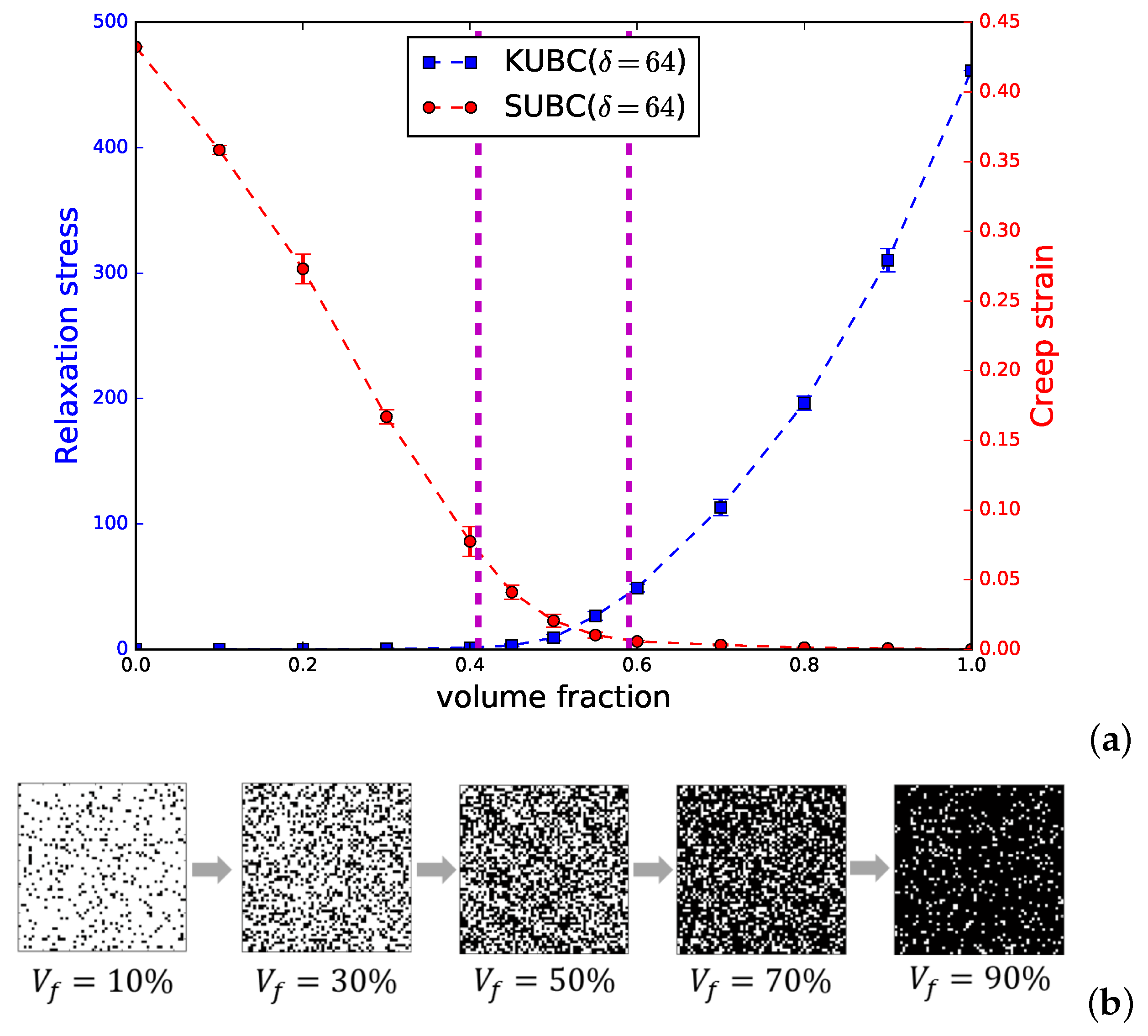
The relaxation stress and creep strain, after stabilization ($t=2$ s), are plotted in Figure 2 for a wide range of volume fractions. When the volume fraction of the viscoelastic phase exceeds ∼60%, the elastic-viscoelastic composite relaxes significantly with much less stress remaining in the body after 2 s under KUBC. Similarly, when the elastic phase occupies more than ∼60%, the composite behaves much more stiffly, and there is a drastic accumulation of specimen strain under SUBC. Both situations show the dominance of the actual percolating phase.

Since the absolute values of the composite’s moduli vary with different volume fractions, it is convenient to normalize the relaxation modulus by the initial value. In this way, all the normalized relaxation moduli scale between 0 and 1, and indicate the relative reduction in the overall stiffness under relaxation. Since a pure elastic material should exhibit no time dependence and sustain a constant modulus under relaxation, the normalized relaxation modulus can be utilized as an indicator of transition from elasticity to viscoelasticity.

The normalized relaxation moduli for all volume fractions are plotted in Figure 3. It is seen that, when the volume fraction of the elastic phase is less than $40\%$ ($v_f>0.59$), the composite shows significant softening after relaxation, which is similar to the viscoelastic matrix. However, once the content of elastic suspension is greater than $60\%$ ($v_f<0.41$), a reduction in stiffness becomes negligible and elasticity dominates the composite’s response. In this case, the damping properties associated with viscoelasticity are almost locked away and do not take effect.

The critical point for Bernoulli site percolation is at $p\simeq 0.59$ [16], so the volume fraction from ≃0.41 to ≃0.59 is the range where a strong transition from an elastic-dominated to a viscoelastic-dominated behavior takes place and a competition between both phases is strongest.

To further quantify this elastic-viscoelastic transition, we propose the parameter relative viscoelasticity, which is calculated by dividing the reduction in normalized modulus in the composite by the maximum possible reduction, and that is the reduction in a normalized modulus if only a pure viscoelastic phase exists. Hence, the relative viscoelasticity for the pure elastic phase is 0, while the relative viscoelasticity for the pure viscoelastic phase is $100\%$.

The relative viscoelasticity is evaluated for the random checkerboard across different volume fraction through Monte Carlo sampling under KUBC. From Figure 4, it can be seen that, for the large contrast of 1000, the mesoscale $\delta =64$ is still not enough for the RVE since the statistical variation exists. At $\delta =128$, a much sharper change in terms of viscoelasticity occurs between the volume fraction $0.41$ and $0.59$. With the viscoelastic phase exceeding $60\%$, more than $90\%$ of the viscoelasticity of the component phase has been incorporated in the composites. This observation is consistent with the percolation theory, which states that the site percolation on the square lattice occurs at the critical probability $p_c\simeq 0.59$.

Note that a sharp change in mechanical response cannot be observed because the elasticity and viscoelasticity are inherently coupled in our model. In the generalized Maxwell model, at least one spring is added, which forces the relaxation stress to be non-vanishing at infinite time. Hence, the constitutive relation of the viscoelastic phase will always be categorized as “solids” as opposed to “fluids”. However, as the relaxation stress after stabilization decreases, the transition slope in Figure 4 tends to become steeper and finally approaches a step shape, which represents the percolation problem of elastic solids and viscous fluids.

3. Fractional Calculus Models in Viscoelasticity

3.1. Background

Considering that the speculations about generalizing the notion of a derivative to non-integer order started with Gottfried W. Leibnitz and Leonhard Euler in the 17th and 18th centuries, the fractional calculus appears to be almost as old as the conventional (Newtonian) calculus. In recent years, significant interest in fractional calculus has been stimulated by applications in physics, engineering, biology, and economics. The mathematical development of fractional calculus is reviewed in many places, e.g., [17,18]. The earliest proponent of fractional calculus in viscoelasticity appears to be Nutting [1], who observed that the stress relaxation phenomenon could be modeled by fractional powers of time. Later, Gemant [2] also found that stiffness and damping properties of viscoelastic materials appeared to be proportional to fractional powers of frequency, which led him to suggest the use of time differentials of fractional order. Bagley and Torvik [3,4] showed that the fractional calculus models of viscoelastic materials are in harmony with the molecular theories that describe the macroscopic behavior of viscoelastic media.

Generalized fractional calculus models for isotropic and anisotropic viscoelasticity are developed and reviewed in [17,18,19]. Compared to classical viscoelasticity, the fractional calculus models of viscoelastic constitutive relations employ derivatives (and integrals) that are of some non-integer order. Constitutive relationships employing derivatives of fractional order relating stress and strain lead to well-posed problems and have evolved as an empirical method of describing properties of many viscoelastic materials, including plastics, polymers, bituminous binder and cartilage [20,21,22,23,24]. Analogous and extensive studies have been conducted in diffusion-wave phenomena [25] and thermoelasticity, typically with an eye to improving the Fourier heat flow model [26]. Overall, a connection of the fractional response model to the underlying material microstructure—be it random or possibly percolating and fractal—is still missing.

3.2. Classical Rheological Models

Classical viscoelastic models require the constitutive relations to be Green’s functions associated with the integer-order derivative in the integral. Starting with

$$\sigma \left(t\right)\sim D^n\left[ϵ\left(t\right)\right]$$

(9)

we have two special cases: (i) when $n=0$, the model is a spring element, whose stress–strain relation is $\sigma \left(t\right)=E$ $ϵ\left(t\right)$; (ii) when $n=1$, the model is a linear viscous dash-pot element: $\sigma \left(t\right)=\eta$ $dϵ\left(t\right)/dt$.

Classical linear viscoelastic material models are represented by a system of springs and dash-pots. Given the support by many experimental observations, one very popular model is the generalized Maxwell model, where a number of Maxwell models are connected in parallel with one isolated spring element introduced for the non-vanishing asymptotic relaxation modulus at infinite time (Figure 5a). Solution of classical linear viscoelastic models leads to exponential type responses. For example, the relaxation modulus for an N-series generalized Maxwell model is expressed as

$$E\left(t\right)=E_0+\sum _{i=1}^n{E}_{i}exp(\frac{-t}{{\tau }_i})$$

(10)

which is also called the Prony series. In a generalized Maxwell model with $N+1$ elements, there is a total of $2n+1$ parameters: $E_0,E_1,{\tau }_1,\dots ,E_n,{\tau }_n$. The advantage of classical rheological models is that exponential functions are easy to handle under mathematical operations such as Laplace and Fourier transforms. However, exponential functions predict a strong frequency dependence of damping properties, whereas measurements of viscoelastic materials reveal a very small change in their dissipative behavior with varying frequency [27]. Thus, classical viscoelastic models have to involve many higher-derivative terms to better agree with measured data, which generally leads to a (much) greater number of material parameters that need to be determined, e.g., [28].

3.3. Fractional Calculus Models

The basic building block of a fractional calculus model in viscoelasticity is a so-called spring-pot described by the equation

$$\sigma \left(t\right)=\eta D^{\alpha }\left[ϵ\left(t\right)\right]$$

(11)

where $\alpha \in (0,1)$ and the (conventionally adopted) fractional derivative of order $\alpha$ of a function $x\left(t\right)$ with respect to time t is given by the Riemann–Liouville definition [29]:

$$D^{\alpha }\left[x\left(t\right)\right]=\frac{1}{\mathsf{\Gamma }(1-\alpha )}\frac{d}{dt}{\int }_0^t\frac{x\left(\tau \right)}{{(t-\tau )}^{\alpha }}d\tau ,0<\alpha <1$$

(12)

where $\mathsf{\Gamma }\left(x\right)$ is the Gamma function. The Fourier transformation of this derivative leads to

$$ϝ\left[D^{\alpha }f\left(t\right)\right]={\left(i\omega \right)}^{\alpha }\tilde{f}$$

(13)

where $\tilde{f}$ is the Fourier transform of function f. In the fractional calculus model, the spring-pot replaces the classical dash-pot of classical viscoelasticity.

Starting with the generalized Maxwell model, there is an additional free parameter of the derivative order ${\alpha }_i$ on each Maxwell model and the total number of parameters increases to $3n+1$. The relaxation modulus of the fractional calculus model in Figure 5b is given by [22]

$$E\left(t\right)=E_0+\sum _{i=1}^n{E}_i{\epsilon }_{\alpha }(-\frac{E_i}{{\eta }_i}{t}^{\alpha })$$

(14)

where

$${\epsilon }_{\alpha }\left(x\right)=\sum _{k=0}^{\infty }\frac{x^k}{\mathsf{\Gamma }(\alpha k+1)}.$$

(15)

Given that the time and frequency dependencies can be reduced with a decreasing derivative order $\alpha$, the viscoelastic behavior of many polymers is generally modeled with fewer parameters using fractional calculus models than in the integer-order models.

4. Fractional Derivative in Elastic-Viscoelastic Composites

One important feature of a fractional calculus model is that it has the flexibility of a continuous passage from a constitutive relation of an ideal solid state to an ideal fluid state. By changing the fractional derivative order $\alpha$ from 0 to 1, the fractional calculus model smoothly transitions from an elastic spring to a viscoelastic dash-pot. This property can be utilized to calibrate the response of viscoelastic random composites.

Now, consider an elastic-viscoelastic composite whose viscoelastic phase is represented by a Zener model ($\alpha =1$); note here that the Zener model has the impact response. Decreasing $\alpha$ from 1 to 0 models the increasing content of the elastic phase. For any intermediate volume fraction of the viscoelastic versus elastic phase, the effective behavior of the composite should be well explained with a four-parameter fractional calculus model of Figure 5b. The corresponding constitutive equation is

$$\sigma \left(t\right)+\frac{\eta }{E_1}\times D^{\alpha }\left[\sigma \left(t\right)\right]=E_0ϵ\left(t\right)+\frac{E_0+E_1}{E_1}\eta \times D^{\alpha }\left[ϵ\left(t\right)\right].$$

(16)

For the elastic-viscoelastic random composite with an arbitrary volume fraction, the behavior of the composite is fully captured by this equation with model parameters $\alpha \in (0,1]$, $E_0$, $E_1$, and $\eta$. Upon taking the Fourier transform of Equation (16), it is seen that this model predicts a frequency-dependent complex modulus of the following form:

$${\displaystyle E^{\ast }\left(\omega \right)=\frac{{\displaystyle E_0+\frac{E_0+E_1}{E_1}\eta {\left(i\omega \right)}^{\alpha }}}{{\displaystyle 1+\frac{\eta }{E_1}{\left(i\omega \right)}^{\alpha }}}.}$$

(17)

Using the relation ${\left(i\omega \right)}^{\alpha }={\omega }^{\alpha }\left[cos(\pi \alpha /2)+isin(\pi \alpha /2)\right]$, the parameters can be fitted by evaluating the loss factor (the tangent of the phase angle $\varphi$) at multiple frequencies [4]:

$${\displaystyle \eta =\frac{{\displaystyle (E_1-E_{0}b)sin\frac{\pi \alpha }{2}{\omega }^{\alpha }}}{{\displaystyle E_0+(E_1+E_{0}b)cos\frac{\pi \alpha }{2}{\omega }^{\alpha }+E_{1}b{\omega }^{2\alpha }}}.}$$

(18)

For a quantitative study, we continue to use the random checkerboard, with responses of the composite at various volume fractions of the viscoelastic phase determined by the computational mechanics model of Section 2. In order to capture the broad range of frequency dependence and obtain a better fit of model parameters, a steady state analysis is performed from $0.01$ to 10 Hz for each composition.

Figure 6 displays the phase angle’s dependencies on frequency, plotted on semi-log and log-log graphs as best fits obtained through a least-squares method. In Figure 6a, we show the case of four volume fractions. In Figure 6b, we display the cases of critical volume fractions (i.e., percolation points) of elastic ($v_f=0.41$) and viscoelastic ($v_f=0.59$) phases; note that $v_f$ pertains to the viscoelastic phase. Simulations have been conducted on $256\times 256$ checkerboard domains, which was the largest size we could handle with our computational resources and allowed us to grasp the RVE-level responses of fractal patterns. At the same time, we considered high contrasts ($1,000$) to grasp the physics of critical phenomena. Overall, the fitted fractional order $\alpha$ is still in the range $[0.99,1.0]$ for low contrast and $[0.98,1.0]$ for high contrast.

Collecting all the results, it was found that, independent of the volume fraction of the viscoelastic phase, the fractional order does not decrease and that the best fit is always practically attained for integer $\alpha$ (=1). The frequency dependence of the elastic-viscoelastic composite remains the same as that of the viscoelastic phase, which is described through classical rheological models. The response of the composite is still in the form of the exponential function

$$E\left(t\right)=E_0+E_1{e}^{-t/b}$$

(19)

and the fitted parameters for different volume fractions are listed in

Table 1. Parameters of fractional calculus model.

Volume Fraction of Elastic Phase	Time Constant $\mathit{b}=\mathit{\eta }/{\mathit{E}}_1$	${\mathit{E}}_0$	$\mathit{\alpha }$
0	$0.25$	$2.0$	1
$0.2$	$0.28$	$2.23$	1
$0.5$	$0.39$	$3.23$	1
$0.8$	$0.51$	$6.06$	1

. It can be seen that adding the elastic phase to the viscoelastic phase only increases the instantaneous modulus $E_0$ and the time constant b, but it does not change the type of the viscoelastic model.

Overall, this study shows that, for one particular viscoelastic composite having a fractal structure but made of classical (non-fractional) viscoelastic continuum phases, the fractional calculus model is not necessary. In other words, the randomness of a composite material—even in the fractal regime (!)—is not the cause of the fractional order viscoelasticity. Rather, it is inferred that such a fractional response must be due to the fractional nature of the constituent phase(s).

5. Conclusions

In this paper, the passage between elasticity and viscoelasticity is investigated in elastic-viscoelastic random composites with strong contrast. For the random checkerboard, a sharp change in response occurs at the volume fraction ∼0.41, with the response switching from a time-independent to a time-dependent type. This critical volume fraction directly corresponds to the probability threshold of site percolation on ${\mathbb{Z}}^2$.

On a separate track, fractional calculus models are applied to describe the change in behavior of the elastic-viscoelastic random checkerboard. Upon examining the whole range of volume fractions, especially at the critical volume fraction, it is found that randomness and fractality of the checkerboard is not the cause of the fractional order viscoelasticity. Therefore, there is at least one random composite material whose response, even at the percolation point having a fractal structure, is adequately described by an integer-order viscoelastic model, which suggests that fractional-order viscoelasticity is likely due to the nature of the constituent phase(s) at the molecular level.

While fractal systems of rheological elements have been studied, they have not been studied from the standpoint of the mechanics of composite materials. Our study shows that a boundary value problem and homogenization in space-time is necessary to obtain an effective constitutive relation. At the same time, models of the aforementioned references are more appropriate for 1D systems. Of course, given that the present study involved one fractal system in 2D, a wealth of other composite media arrangements in 2D and 3D still needs to be analyzed to arrive at general conclusions to the question posed in the title.