Article

Evidential K-Nearest Neighbors with Cognitive-Inspired Feature Selection for High-Dimensional Data

by
Yawen Liu
1,
Yang Zhang
1,*,
Xudong Wang
2 and
Xinyuan Qu
3
1
School of Electronic and Information Engineering, Beijing Jiaotong University, Beijing 100044, China
2
Unicom Digital Technology Co., Ltd., Beijing 100032, China
3
Resource Environment Tourism College, Capital Normal University, Beijing 100048, China
*
Author to whom correspondence should be addressed.
Big Data Cogn. Comput. 2025, 9(8), 202; https://doi.org/10.3390/bdcc9080202
Submission received: 13 June 2025 / Revised: 15 July 2025 / Accepted: 1 August 2025 / Published: 6 August 2025

Abstract

The Evidential K-Nearest Neighbor (EK-NN) classifier has demonstrated robustness in handling incomplete and uncertain data; however, its application in high-dimensional big data for feature selection, such as genomic datasets with tens of thousands of gene features, remains underexplored. Our proposed Granular–Elastic Evidential K-Nearest Neighbor (GEK-NN) approach addresses this gap. In the context of big data, GEK-NN integrates an Elastic Net within the Genetic Algorithm’s fitness function to efficiently sift through vast amounts of data, identifying relevant feature subsets. This process mimics human cognitive behavior of filtering and refining information, similar to concepts in cognitive computing. A granularity metric is further employed to optimize subset size, maximizing its impact. GEK-NN consists of two crucial phases. Initially, an Elastic Net-based feature evaluation is conducted to pinpoint relevant features from the high-dimensional data. Subsequently, granularity-based optimization refines the subset size, adapting to the complexity of big data. Before applying to genomic big data, experiments on UCI datasets demonstrated the feasibility and effectiveness of GEK-NN. By using an Evidence Theory framework, GEK-NN overcomes feature-selection challenges in both low-dimensional UCI datasets and high-dimensional genomic big data, significantly enhancing pattern recognition and classification accuracy. Comparative analyses with existing EK-NN feature-selection methods, using both UCI and high-dimensional gene datasets, underscore GEK-NN’s superiority in handling big data for feature selection and classification. These results indicate that GEK-NN not only enriches EK-NN applications but also offers a cognitive-inspired solution for complex gene data analysis, effectively tackling high-dimensional feature-selection challenges in the realm of big data.

1. Introduction

As a foundational model in machine learning, K-Nearest Neighbors (K-NN) [1] is appreciated for its simplicity and effectiveness. Innovations such as the Evidential K-Nearest Neighbors (EK-NN), which integrates Evidence Theory [2], have enhanced K-NN’s capabilities, particularly in managing uncertainty in data. Dempster–Shafer (DS) Evidence Theory has been widely adopted within EK-NN models [3,4,5] to better leverage information uncertainty for decision-making. The EK-NN classifier treats each neighbor of the target “x” as a source of evidence regarding the class membership of “x”, quantified via a mass function. This mass function is adjusted based on each neighbor’s proximity to “x”, with the final classification determined by synthesizing these functions according to Dempster’s rule [6].
Due to its robust handling of incomplete and uncertain data, the EK-NN classifier has found applications in fields like machine learning and pattern recognition [7,8,9]. Over the years, enhancements have been proposed to improve EK-NN, including alternative combination rules for evidence, parameter optimization using gradient and evolutionary algorithms [10,11], and adaptive models that recalibrate feature space and determine optimal K-values [12]. Other EK-NN variants include hybrid classification rules [13], evidence instance selection [14], multimodal perturbation [15], augmented integration [16], and contextual discounting approaches [17]. Despite these advancements, the feature-selection challenge remains underexplored in EK-NN, especially in high-dimensional contexts such as gene data classification, where dimensionality can overwhelm traditional methods. Although recent research in K-NN has produced feature-selection methods such as hybrid filter–wrapper approaches [18] and prototype selection combined with feature weighting [19], similar techniques for EK-NN are lacking. In the broader context of feature selection, foundational work by Guyon and Elisseeff [20] established core principles for assessing feature relevance and redundancy, forming the theoretical basis for many subsequent algorithms in high-dimensional analysis. Building on this, recent developments have explored more advanced paradigms. For instance, Deep Feature Selection (DFS) [21] integrates deep neural architectures with embedded sparsity constraints to simultaneously capture nonlinearity and perform input-level feature pruning, especially useful in genomic sequence modeling. Variational dropout-based approaches [22] provide a Bayesian framework for automatic sparsification by assigning individualized dropout rates per weight, achieving substantial model compression while preserving accuracy. Reinforcement learning-based methods [23] conceptualize feature selection as a sequential decision process, introducing Monte Carlo Tree Search techniques to iteratively explore informative subsets with theoretical guarantees. While these methods demonstrate effectiveness in general-purpose classification tasks, they are primarily designed for deterministic learning models and do not account for uncertainty in feature contribution. As a result, their direct applicability to evidence-theoretic frameworks like EK-NN remains limited. In contrast, EK-NN leverages Dempster–Shafer theory to model evidential uncertainty, which is particularly beneficial in domains such as gene expression analysis or medical diagnostics, where data is often noisy, sparse, or partially labeled. Therefore, developing feature-selection mechanisms within EK-NN is essential for enabling both robust inference and interpretable decision-making in such high-dimensional, uncertainty-prone contexts.
Addressing feature selection within EK-NN is particularly valuable for high-dimensional gene datasets, where selecting optimal feature subsets is critical for improving classification accuracy and efficiency. Prior studies, such as those by Lian [24] and Su [25], have used Genetic Algorithms and rough set theory for feature selection within EK-NN. Yet, they face challenges with high-dimensional data [25] and the risk of local optima.
To address the challenge of high-dimensional datasets, GEK-NN incorporates a Genetic Algorithm (GA) to effectively explore feature subsets, combined with an Elastic Net embedded in the GA’s fitness function. This integration allows GEK-NN to streamline irrelevant features, significantly reducing the dimensionality and complexity of the data while maintaining the relevance of selected features for classification. To tackle the risk of local optima, GEK-NN leverages the optimization capabilities of the Genetic Algorithm, which employs crossover and mutation operations to enhance the search space exploration. Additionally, a granularity metric is introduced to guide the GA further in optimizing the compactness and effectiveness of feature subsets. This dual approach ensures that the GA avoids premature convergence, effectively escaping local optima while refining feature subset quality.
The GEK-NN algorithm progresses through two main phases: (1) Elastic Net-based evaluation of features, enabling rapid elimination of redundant features, and (2) granularity-informed optimization that steers the GA towards compact, high-quality subsets. By integrating these elements, GEK-NN addresses critical challenges in high-dimensional feature selection and provides a robust method for EK-NN applications in gene dataset classification.
This paper’s contributions are summarized as follows: (1) Integration of Elastic Net into the GA’s fitness function, enhancing feature assessment and pruning. (2) Incorporation of a granularity metric to prioritize compact and effective feature sets. (3) Improved global search capabilities within the GA, ensuring thorough exploration and reliable identification of optimal feature subsets for high-dimensional gene datasets. (4) Comprehensive experiments were conducted on standard UCI datasets and high-dimensional gene datasets to evaluate the performance of EKNN-based feature-selection algorithms. Additionally, a detailed comparison of EK-NN’s classification accuracy using different feature subsets demonstrates the effectiveness and validity of the proposed GEK-NN approach.
The structure of the paper is as follows: Section 2 Preliminaries provides an overview of Genetic Algorithms and EK-NN classifiers. Section 3 GEK-NN Implementation Method presents the details of the GEK-NN algorithm, including the incorporation of Elastic Net and the design of the fitness function. Section 4 Experimental Results evaluates the performance of GEK-NN on UCI datasets as well as high-dimensional gene datasets. Finally, the Section 4.5 Conclusions summarizes the key findings of the study.

2. Preliminaries

2.1. Genetic Algorithm

The Genetic Algorithm (GA), initially introduced by John Holland [26], is rooted in the principles governing evolutionary processes observed in nature. Genetic Algorithms find extensive applications across domains such as combinatorial optimization, machine learning, signal processing, adaptive control, and artificial life [27]. There are also many applications of Genetic Algorithms for feature selection [28,29]. The steps for implementing the Genetic Algorithm are as follows.
Individual encoding and Initial population. The encoding process of initializing a population can be described using mathematical formulas. Each individual is represented by a string of binary codes, known as a chromosome. Let N be the number of individuals in the population, and n be the length of the binary code for each individual. Each I i can be represented as
I i = b i , 1 , b i , 2 , , b i , n , b i , j { 0 , 1 }
Each b i , j represents a binary bit, and it can be randomly generated or initialized. This way, each individual is represented by a binary string of length n, forming the entire initial population. The initialization process of the population involves generating N such binary strings, which can be formulated as:
I n i t i a l i z e   Population = { I 1 , I 2 , . . . , I N }
Fitness function. The fitness function evaluates and scores individuals in each generation and is designed to align with the feature-selection requirements. It reflects the performance of an individual, with better-performing individuals more likely to be selected as “good parents” and retained for the next generation. Create the next generation:
  • Selection: Genetic operators are used to create the next generation. Elite individuals are selected as parents based on their fitness values, and offspring are generated through crossover and mutation. Individuals with higher fitness are more likely to be selected, mimicking the principle of survival of the fittest in natural selection. To ensure consistent generation size, Equation (3) must be satisfied:
    ( B S + R S ) 2 × c h i l d r e n = i n i t i a l   p o p u l a t i o n   s i z e
    BS is the number of individuals selected as the best, RS is the number of randomly selected individuals, children is the number of offspring produced by each pair of parents, and the initial population size is the size of the initial population.
  • Crossover: A pair of individuals is selected from the previously selected parents, and a crossover operation is performed to generate new individuals. This study employed the single-point crossover technique.
  • Mutation: After crossover, individuals in the current population are replaced. The new individuals undergo mutation to introduce genetic variations.
  • Stopping Criteria: Common stopping criteria in Genetic Algorithms include reaching a set number of iterations or observing no improvement in the fitness function over consecutive generations. In this experiment, the criterion of a fixed number of iterations is applied.

2.2. Evidential K-NN

Dempster–Shafer theory. Given a frame of discernment Θ = { θ 1 , θ 2 , , θ c } , a mass function is defined as a mapping from 2 Θ to [0,1] such that
{ A 2 [ Θ ] } m ( A ) = 1 m ( ) = 0
If m ( A ) > 0 , then A is said to be a focal element. m ( A ) represents the confidence that the test target belongs to the proposition A, rather than a subset containing A. Evidence Theory provides Dempster rules [3] that orthogonally combine information from multiple independent sources to realize the fusion of multiple pieces of evidence. Let m 1 and m 2 be two basic probabilistic assignment functions defined in the same discriminative framework, and the formula for the combination rule is as follows:
m D S ( C ) = A B = C m 1 ( A ) m 2 ( B ) 1 A B = m 1 ( A ) m 2 ( B ) m ( ) = 0
m DS ( C ) is the evidence obtained after fusing evidence m 1 and m 2 . Define the conflict coefficient K as
K = A B = m 1 ( A ) m 2 ( B )
K is a conflict coefficient used to measure the degree of conflict between pieces of evidence. A larger K indicates a greater conflict between the evidence, and if K = 1 , the combination rule cannot be used. After all pieces of evidence have been combined, the pignistic probability distribution associated with a mass function m can be defined by
B e t P ( θ ) = { A Θ | θ A } m ( A ) | A |
for all θ Θ . Decisions are made based on the results of pignistic probability, and the category containing the maximum probability is the decision category.
EK-NN algorithmic principle. In the EK-NN model, it is assumed that there is a set of training data as T R . The corresponding frame of discernment Θ = { θ 1 , θ 2 , , θ c } . The training set T R = x 1 , θ ( x 1 ) , x 2 , θ ( x 2 ) , , x n , θ ( x n ) consists of n samples, x i R D × 1 = ( x i 1 , x i 2 , , x i D ) is a D -dimensional feature vector. θ ( x i ) Θ indicates the category to which x i belongs in the category framework. A test sample is denoted as a D-dimensional vector y t . According to the number of nearest neighbors K in EK-NN, the domain space of the samples in the test set y t is defined as N K ( y t ) , and each individual in this space provides evidence for the class membership of the test sample y t . The evidence from a neighbor x t ( j ) q belonging to class θ q is formalized as a mass function m t · x t ( j ) q .
m t θ q x t ( j ) q = α e x p γ m t · x t ( j ) q y t 2 2 m t Θ x t ( j ) q = 1 α e x p γ m t · x t ( j ) q y t 2 2
where α is a constant such that 0 < α 1 (usually α = 0.95 ) , γ is the discount parameter ( γ = 1 for all q for simplicity) [25]. Equation (8) shows that as the distance between y t and x t ( j ) q increases, x t ( j ) q provides less evidence that the test samples are pointed to as belonging to the category θ q , and the residual information is assigned to the ignorant class Θ . The final y t mass function is computed by the
m t = x t ( j ) N K ( y t ) m t · | x t ( j )
Evidence fusion based on K pieces of evidence from N K ( y t ) using Equation (9). Then, y t is classified by taking the maximum value of the mass function for each class.
θ ^ ( y t ) = arg max θ Θ m t ( θ q )

3. GEK-NN Implementation Method

In this section, we elaborate on the algorithmic structure of GEK-NN and the associated experimental parameters. The proposed framework consists of two primary stages: (A) feature selection based on a Genetic Algorithm integrated with Elastic Net and granularity constraints, and (B) classification through an EK-NN model. The complete workflow of GEK-NN is illustrated in Figure 1.
Cognitive-Inspired Motivation. The design of GEK-NN draws inspiration from cognitive mechanisms underlying human decision-making, particularly the heuristic process of managing complexity and uncertainty in high-dimensional environments. Specifically, the GA component reflects the principle of divergent thinking, wherein the human brain explores multiple candidate solutions or strategies in parallel when faced with a problem space. This enables the discovery of diverse and potentially innovative feature subsets. Complementing this, the embedded Elastic Net functions as a convergent filtering mechanism, akin to how humans narrow down choices based on error signals or task relevance. It selectively emphasizes discriminative features while suppressing irrelevant or redundant information, mimicking the cognitive process of focusing attention on the most informative cues. Furthermore, the notion of granularity is introduced to simulate the concept of bounded rationality—a key idea in cognitive science that reflects the limited capacity of human working memory and decision scope. By penalizing overly large feature subsets, the model encourages concise yet effective representations, aligning with the cognitive preference for simplicity and efficiency.
Technical Overview. In the feature-selection phase (Part A), the GA framework evolves candidate feature subsets across generations. The fitness of each subset is evaluated using a dual-objective function that combines root mean square error (RMSE) from the Elastic Net with a granularity metric reflecting feature sparsity. This balance ensures that the selected subset is not only predictive but also compact. After iterative optimization, the most promising feature subset is passed to the classification module (Part B). The EK-NN classifier integrates evidential information from neighboring instances and resolves uncertainty using a confusion-matrix-based reliability measure. Dempster–Shafer theory is then employed to fuse multiple sources of evidence and make a final decision, offering robustness in ambiguous or noisy data scenarios.

3.1. Genetic Algorithm Execution Process

Based on the Genetic Algorithm framework, the initialization parameters of the Genetic Algorithm are shown in Table 1. Assuming that the chromosomes of an initial population consist of C = ( C 1 , C 2 , , C i , , C P s i x e ), C i = ( b 1 , b 2 , , b m ) , i { 1 , 2 , , P size } . b j 0 , 1 , where 1 indicates that the location feature is selected and 0 indicates the opposite. Each C i represents a way of selecting feature combinations. F ( C i ) f i Ω , where F denotes fitness function, Ω represents the universal set of values taken by f i , f i denotes the fitness value of the chromosome C t , the aim is to find an optimal C t that minimizes the fitness value f t .
In the fitness function, Elastic Net and granularity guide the Genetic Algorithm towards effective feature selection. Elastic Net uses RMSE to measure feature accuracy, removing less important features to enhance classification performance, while granularity helps identify effective feature subsets efficiently. The Elastic Net regularization, an adaptation of multiple linear regression, uses L1 and L2 penalties to select important variables and improve prediction accuracy, akin to a fishing net that retains significant predictors while discarding irrelevant ones [30,31,32].
Definition 1
(Elastic Net). Suppose a multivariate linear regression model (Equation (11)):
Y = X β ^ + ε
Y is the response variable (target), X is the design matrix containing all the feature variables, β ^ is the coefficient vector to be estimated, ε is the error term. Suppose that we have p = 1 , . . . , P predictors denoted by x 1 , . . . , x p , an estimate of the response variable Y can be modeled as Y ^ = β 0 + β 1 x 1 + + β P x p , based on linear regression. The coefficients ( β ^ = [ β 0 , . . . , β P ] ) are calculated by minimizing the sum of the squares of the error residuals. The objective function for Elastic Net can be written as:
min 1 2 m     Y X β ^   2 2 + λ 1     β ^   1 + λ 2     β ^   2 2
  β ^   1 = p = 0 P | β p | ,   β ^   2 = p = 0 P β p 2
The first term minimizes the sum of squared residuals for fitting the data. λ 1   β ^   denotes the L1-norm, promoting sparsity in coefficients and encouraging some coefficients to become zero, achieving feature selection. λ 2   β ^   2 2 denotes the L2-norm, controlling the sum of squared coefficients to prevent overfitting. According to Fatemeh and Hu [33], Elastic Net is used innovatively in the fitness function by combining Lasso and Ridge Regularizations, which reduces the coefficients of uncorrelated features and retains correlated ones for effective feature selection [34]. The optimal values of λ 1 and λ 2 were determined using a comprehensive grid search strategy, in alignment with the parameter selection methodology proposed in [33]. Specifically, we defined a logarithmically spaced search grid for both λ 1 and λ 2 over the interval [ 10 4 , 10 1 ] . For each ( λ 1 , λ 2 ) pair in the grid, ten-fold cross-validation was conducted on the training dataset. In each fold, the Elastic Net model was trained on nine subsets and evaluated on the remaining one using root mean squared error as the performance metric. The average RMSE across the ten folds was calculated, and the parameter combination yielding the lowest mean RMSE was selected as the optimal regularization configuration. This procedure enables a principled trade-off between sparsity and coefficient shrinkage, thus enhancing the model’s generalization capability.
The fitness function employs global metrics, namely RMSE, and granularity, to provide comprehensive assessments across the dataset. RMSE, computed using Elastic Net, evaluates prediction accuracy. Granularity assesses the extent to which the selected features adequately cover the feature space, ensuring they capture the essential variations in the data necessary for accurate predictions.
Definition 2
(RMSE). The training set, with n samples as T R = { ( x i , y i ) i = 1 , 2 , , n } , uses actual values y i and predictions y i ^ . Each of the k folds is tested once. The average R M S E C V over k-fold validation estimates the algorithm’s performance (Equation (14)).
R M S E C V = 1 # f o l d s 1 # f o l d s 1 n i = 1 n ( y i y i ^ ) 2
The second global concept introduced in the fitness function is granularity. In prior research penalty factors have often been applied to restrict the size of the feature subset selected [33]. However, simply considering the absolute number of features in the subset does not adequately reflect its proportion relative to the entire feature space. The concept of granularity provides a more accurate relative measure. Within the framework of Genetic Algorithms, granularity is utilized to influence the selection process toward preferring individuals that encompass a smaller number of features, achieved through iterative rounds [35].
Definition 3
(Granularity). Assuming that P is the population of the current generation, U consists of all genes, and U / P = { S 1 , S 2 , , S K } , where S K is the subset of selected features in the chromosome containing the kth entry, and U / P denotes that it is all the selected genes in the population of the current generation; then, the combination granularity G ( C i ) and the average combination granularity G p ( C ) are defined as (Equations (15) and (16)):
G ( C i ) = | S i | | U | log 2 | S i | | U |
G p ( C ) = 1 K i = 1 K G ( C i )
If | S K | = 1 , it means that the K t h chromosome selects the least number of genes, selects the least number of features, and the average combinatorial granularity of G P ( C ) reaches the maximum log 2 | U | / | U | ; if | S K | = | U | , it means that the Kth chromosome selects all genes, selects all the features, and the average combined granularity of G p ( C ) reaches a minimum of 0. It is easy to determine that 0 G p ( C ) log 2 | U | / | U | .
Definition 4
(Fitness Function). The Genetic Algorithm for feature selection uses a fitness function based on RMSE and granularity to identify the best individuals in each iteration. Elastic Net removes redundant features, retaining the most valuable ones. Features frequently appearing in optimal subsets are selected for the final subset. The process aims to reduce RMSE and increase granularity over iterations, as reflected in the fitness function.
F G A = r R M S E w g G ( C )
r RMSE denotes the value of the model error obtained using the subset of features corresponding to the genetic code of the individual in the current offspring; G ( C ) denotes the granularity, i.e., the proportion of selected features in the current individual. To balance the influence of model accuracy and feature compactness, a weighting factor w g is introduced in front of the granularity term in the fitness function. While the granularity is expected to be increasingly emphasized to encourage feature reduction, its contribution must not dominate the fitness evaluation. Therefore, an appropriate setting of w g is crucial. In this study, we adopt w g = 0.15 as the default setting. This value is not arbitrarily chosen; it has been empirically validated through a series of parameter sensitivity experiments, as detailed in Section 4.2. These experiments evaluate the performance of GEK-NN under different w g values across multiple datasets, and demonstrate that w g = 0.15 consistently provides an optimal trade-off between classification accuracy and feature sparsity. Thus, this setting ensures that the granularity term contributes appropriately to the overall fitness assessment, maintaining a balance between prediction performance and subset compactness in the Genetic Algorithm’s optimization process.
Definition 5
(Fitness Function Optimization Problem). Given the fitness function F G A , the optimization problem is to find the chromosome B such that:
B = arg min C i P F G A ( C i )
P is the population of chromosomes.
Given a fitness function F G A : Ω R . Genetic Algorithm converges to a feature subset B Ω optimizing F G A .
Proof. 
We establish the convergence of the proposed algorithm by modeling its dynamics as a time-homogeneous Markov chain and invoking classical convergence results. Let { X t } t 0 be the sequence of population states generated by the algorithm, where X t Ω denotes the population state at iteration t, and Ω is the finite state space of all admissible populations (candidate solutions). The transition probability P ( X t + 1 = B X t = B ) defines a Markov process governed by the evolutionary operators (selection, crossover, mutation).
(1) Irreducibility. We assume that the mutation operator has a strictly positive probability p m > 0 of perturbing any individual to any other feasible form, possibly across multiple generations. Therefore, for any two population states B , B Ω , there exists an integer n such that the n-step transition probability P n ( B , B ) > 0 . Hence, the Markov chain is irreducible.
(2) Aperiodicity. Due to the possibility of remaining in the same state (e.g., through reproduction without change or acceptance under selection), we have P ( B , B ) > 0 for all B Ω . This implies that the period of each state is 1, and thus the chain is aperiodic.
(3) Existence of stationary distribution. Since the chain is both irreducible and aperiodic over a finite state space, it admits a unique stationary distribution π satisfying:
lim t P t ( · μ ) π = 0 ,
for any initial distribution μ .
(4) Convergence toward optimal solution. The selection mechanism embedded in the algorithm biases the transition probabilities toward higher-fitness states: if F G A ( B ) > F G A ( B ) , then
P ( X t + 1 = B X t = B ) > P ( X t + 1 = B X t = B ) .
Therefore, the stationary distribution π places higher mass on states with larger F G A values. Let B = arg max B Ω F G A ( B ) denote the globally optimal state. Then, π ( B ) > 0 , and we have:
lim t P ( X t = B ) = π ( B ) = max B Ω π ( B ) ,
which implies that the algorithm converges in probability toward the optimal population state B . □
Each chromosome C i is scored using a fitness function. The T R is selected for input using the combination of feature selections represented by each chromosome C t . After scoring all individuals of the current generation, the optimal result B is outputted by continuous iteration according to the flow of the Genetic Algorithm.

3.2. Classification Based on EK-NN Model

Suppose the optimal feature subset of the output is B ( B B ) . B represents the universal set of all feature data. Use some of the raw data indexed in B as input data for the EK-NN model and use the EK-NN model for classification. Training the original KNN model using the T R set, then inputting the test data indexed by the optimal feature subset y t , B to get its domain N K ( y t , B ) .
Definition 6
(Nearest Neighborhood). For a test sample y t , B the nearest neighborhood N K ( y t , B ) is formally defined as:
N K y t , B = { x 1 , x 2 , . . . , x K T R }
where T R is the training set and each x i is selected such that:
Δ x i , y t , B Δ x j , y t , B , x j { x 1 , x 2 , . . . , x K }
with Δ being the chosen distance metric (e.g., Euclidean). The set c signifies the full set of features, K is the number of nearest neighbors considered.
Definition 7
(Mass Function). The membership contribution of each training sample x t , B ( j ) q in N K ( y t , B ) is quantified by a mass function, which provides evidence towards the class θ q to which x t , B ( j ) q belongs. This is mathematically described by:
m t , B θ q x t , B ( j ) q = α exp γ x t , B ( j ) q y t , B 2
m t , B Θ x t , B ( j ) q = 1 α exp γ x t , B ( j ) q y t , B 2
Here, α and γ are predefined constants, and x t , B ( j ) q y t , B 2 is the squared Euclidean distance between the two D-dimensional vectors. Each nearest neighbor produces an evidence for the classification of the test sample that indicates the probability that the sample belongs to the labeling category of that nearest neighbor, and then using DS rules to fuse these evidences to obtain the probability that the sample belongs to the labeling category.

3.3. GEK-NN Classification Procedure and Time Complexity

Initializing a population of N chromosomes, each with L features, has a complexity of O ( N · L ) . Assuming each fitness evaluation per chromosome costs O ( L ) , the total for evaluating the entire population is O ( N + L ) . In the process of selection, it typically runs in O ( N log N ) . In crossover, it is implemented per individual, costing O ( L ) per crossover event, with a total for an individual being O ( N · L ) . In mutation, with a mutation probability p m , the expected complexity is O ( p m · N · L ) . Thus, the per-generation complexity of GA can be summarized as O ( N · L + N log N + N . L + p m · N · L ) , which simplifies to O ( T · N · L ) for T generations, assuming p m and sorting are not dominant.
Assuming Elastic Net reduces the feature count from L to L . Crossover reduced to O ( N + L ) . Mutation reduced to O ( p m · N · L ) . The reduction in complexity due to the reduced feature set L from using Elastic Net.
Crossover Complexity Reduction:
Δ C cross = O N · ( L L )
Mutation Complexity Reduction:
Δ C matate = O p m · N · ( L L )
Total Reduction:
Δ C total = O ( 1 + p m ) · N · ( L L )
Integrating Elastic Net into GA not only potentially speeds up the convergence by focusing the genetic operations on a reduced, more relevant set of features but also significantly reduces the computational complexity of the crossover and mutation processes. This reduction is particularly beneficial in scenarios with large L where L L represents a substantial decrease in feature count, leading to efficiency gains in the genetic operations within GA.

4. Experimental Results

In this section, datasets validate GEK-NN’s performance: low-dimensional UCI datasets first demonstrate its general applicability to conventional data scales, while high-dimensional genomic datasets take center stage to highlight its exceptional capabilities in extreme feature spaces. The UCI datasets (Table 2 [36]), with moderate feature dimensions, serve as a baseline for cross-domain robustness, whereas genomic datasets from Keng Ridge [37] and KEEL [38] (Table 3), featuring tens of thousands of gene-level features, embody complexity, noise, and the “curse of dimensionality”—challenges where GEK-NN’s unique value emerges. Post-preprocessing, we applied 10-fold cross-validation with ten independent repetitions (repeated 10 × for 10-fold CV) on each genomic dataset to mitigate the effects of high dimensionality and stochasticity. In each repetition, data were randomly reshuffled and split into ten folds. This yielded a total of 100 evaluation runs per model. Final accuracy values are reported as the mean ± standard deviation across these runs.
Implementation Details. All experiments were conducted on a standard personal computer equipped with an Intel Core i5 CPU (2.4 GHz), 16 GB RAM, and no GPU acceleration, running the Windows 10 operating system. The proposed GEK-NN algorithm was implemented in Python 3.7, utilizing open-source libraries including scikit-learn, NumPy, and DEAP for machine learning models, numerical computation, and evolutionary algorithms, respectively. Since the primary computational task of GEK-NN lies in wrapper-based feature selection and classification on high-dimensional genomic data (often containing tens of thousands of features), the method is designed to operate efficiently on conventional CPU-based hardware. All experiments were completed within reasonable runtimes, demonstrating the practical feasibility and accessibility of the approach without reliance on specialized computing resources. In all experiments, the EK-NN component in GEK-NN adopts the Euclidean distance metric. The confidence discount parameter α was set to 0.95, and the discounting coefficient γ was fixed at 1 across all classes, following the standard formulation in [25]. These parameters were empirically validated and kept constant across all datasets for consistency and reproducibility.

4.1. An Illustrative Example (Seeds)

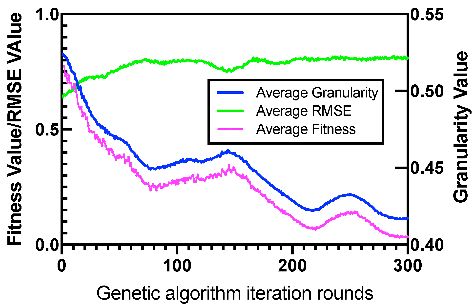
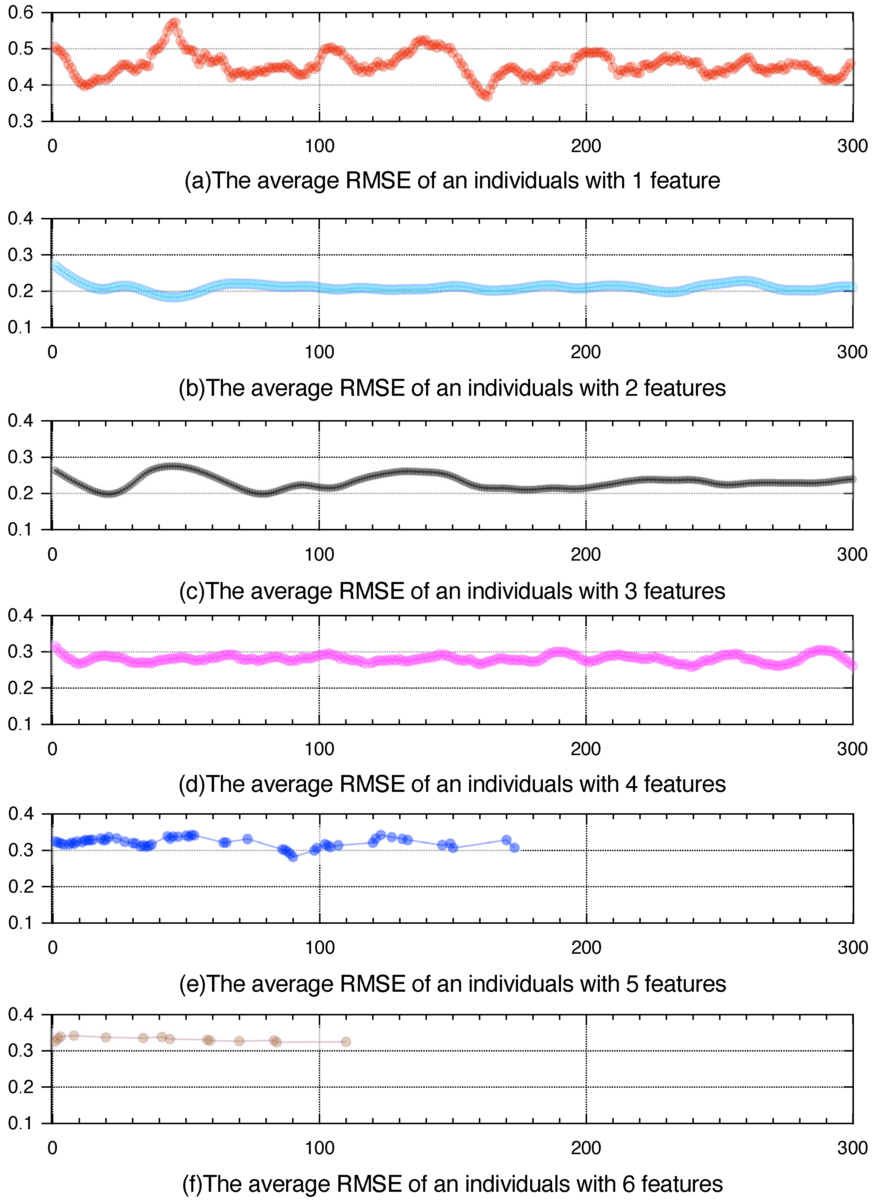
We use the Seeds dataset as an illustrative example. In the feature-selection process, granularity increases and converges with iterations, aligning with the algorithm’s goal; fewer features yield higher granularity (Figure 2). Simultaneously, the average RMSE decreases, indicating improved feature fitting accuracy. The fitness function converges after a steady decline, confirming that the model effectively selects the optimal feature subset. Over 300 iterations, individuals with two or three features, shown to have lower RMSE values (Figure 3), are favored in later stages, undergoing further crossover and mutation to form optimal subsets. Despite individuals with one or four features persisting, their higher RMSE results in lower selection frequency (Figure 4). The final optimal subset is B = ( 2 , 7 ) , with B = ( 1 , 2 , 7 ) as sub-optimal, filtered via Elastic Net to eliminate unnecessary features. Selecting the two-feature subset confirms that higher granularity correlates with better classification. Cross-validation identifies the optimal K = 8, with EK-NN achieving 0.9643 accuracy using B = ( 2 , 7 ) , compared to 0.8928 with all features, indicating that selective features enhance accuracy.
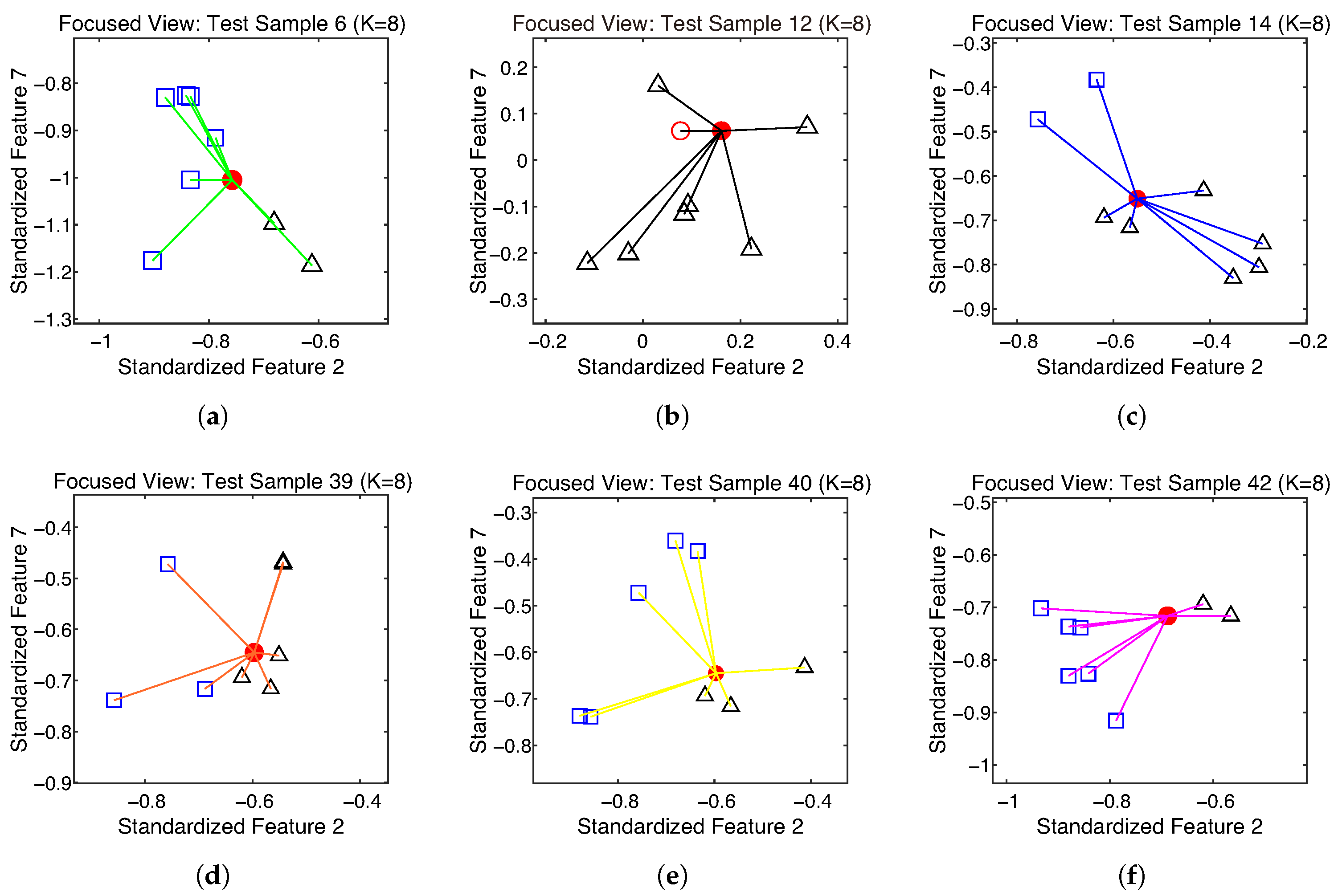
The ordinary KNN algorithm achieves an accuracy of 0.9286, while the GEK-NN algorithm performs better by utilizing nearby information more comprehensively. Unlike KNN, which averages neighbor votes and may lose inter-category relationships, GEK-NN combines evidence from each neighbor through a confusion matrix and DS rule, then selects the category with the largest evidence based on maximum pignistic probability. In Figure 5, samples misclassified by KNN but correctly classified by EK-NN demonstrate this: squares represent category ω 1 , triangles represent ω 2 , and circles represent ω 3 . For instance, samples 6, 14, and 39 are correctly classified by using the relationship among categories, while conflicting cases like samples 12, 40, and 42 are resolved accurately by EK-NN adjustments.

4.2. Parameter Sensitivity Analysis

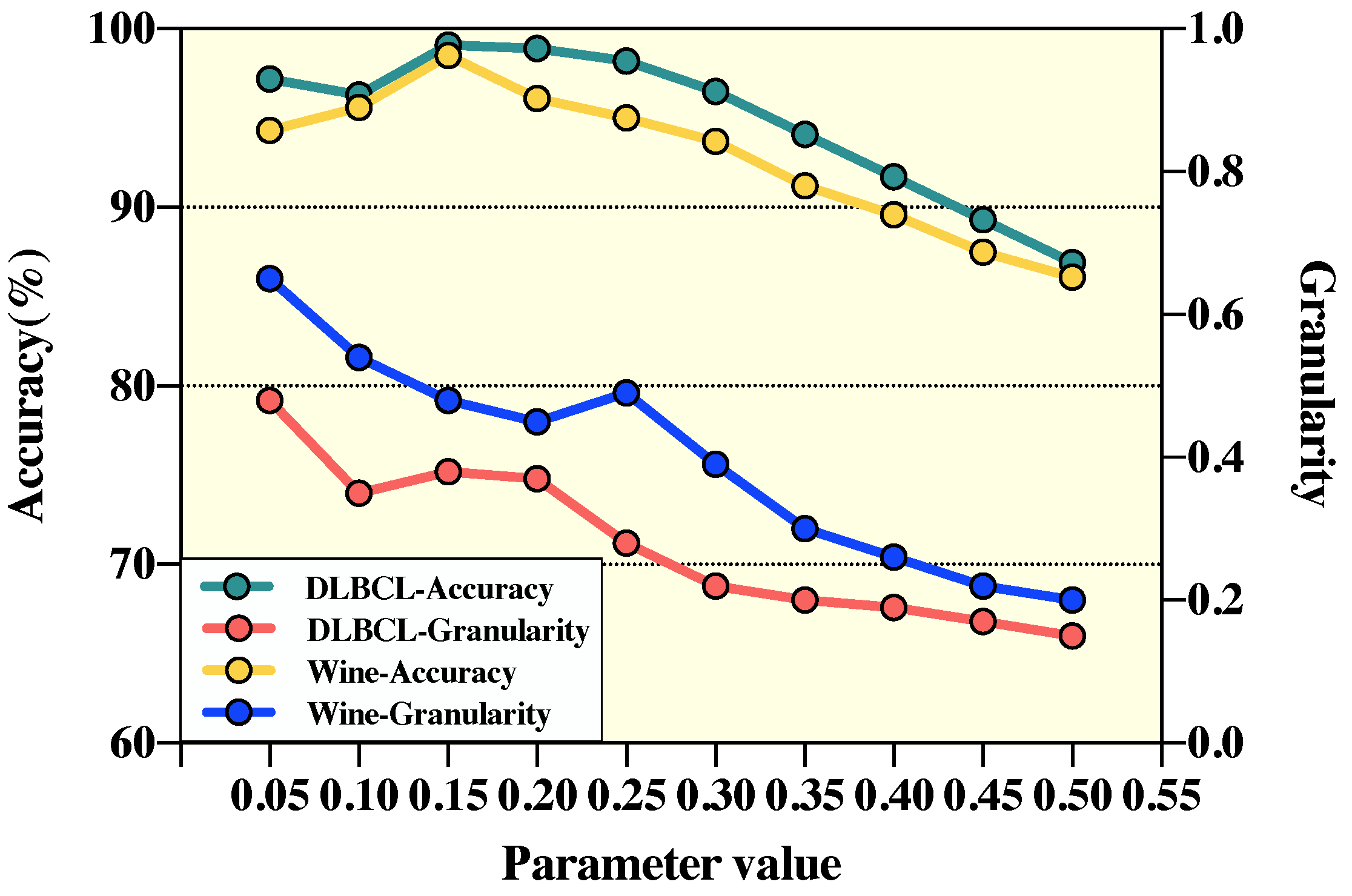
Sensitivity Analysis of the Weighting Factor. To justify the choice of w g , we conducted a comprehensive sensitivity analysis, varying w g from 0.05 to 0.50 in increments of 0.05. The results, summarized in Table 4 and illustrated in Figure 6, show the corresponding changes in classification accuracy and granularity on two representative datasets: Wine (UCI dataset) and DLBCL (high-dimensional gene dataset). These plots reveal the performance trends as w g varies, offering insights into its influence on the GEK-NN model.
The best performance is consistently observed when w g is in the range of [ 0.10 ,   0.20 ] , with w g = 0.15 achieving the highest accuracy (98.5% on Wine and 99.1% on DLBCL) while maintaining relatively high granularity values (0.48 and 0.38, respectively), indicating a compact yet effective feature subset. This confirms that w g = 0.15 offers a robust and well-balanced configuration, striking a favorable trade-off between minimizing model error and reducing feature dimensionality.
Notably, the model performance remains stable within this range, suggesting that GEK-NN is not overly sensitive to small fluctuations in w g . This robustness is desirable in real-world applications, where fine-tuning may not always be feasible. Based on our observations across multiple datasets, we recommend setting w g = 0.15 as a practical default. In tasks that demand extreme accuracy or higher sparsity (e.g., embedded or resource-constrained systems), w g can be slightly adjusted within the stable zone ( [ 0.10 ,   0.20 ] ) to suit specific needs. Overall, this analysis provides empirical evidence that granularity, when appropriately weighted, significantly enhances the model’s generalization ability without overfitting or feature overuse.
Evaluating w g across Low- and High-Dimensional Scenarios. To ensure the effectiveness of the fitness function across datasets with varying levels of model error, we normalize the RMSE term r RMSE into the [ 0 ,   1 ] range prior to its inclusion in the objective function. This normalization allows it to be on a comparable scale with the granularity term G ( C ) , which naturally lies within [ 0 ,   1 ] . As a result, the weighting factor w g does not serve to rescale disparate quantities, but rather plays the role of a trade-off controller—determining the relative importance of feature sparsity versus predictive accuracy in the evolutionary optimization process. To evaluate the robustness of w g , we conducted experiments on datasets with significantly different RMSE profiles, including low-dimensional UCI datasets (Wine) and high-dimensional genomic datasets (DLBCL), where error values naturally differ due to intrinsic data complexity. The results, summarized in Table 4, demonstrate that w g = 0.15 consistently yields strong accuracy and compact feature subsets, confirming the generalizability of the fitness function across diverse data regimes.

4.3. Performance of GEK-NN

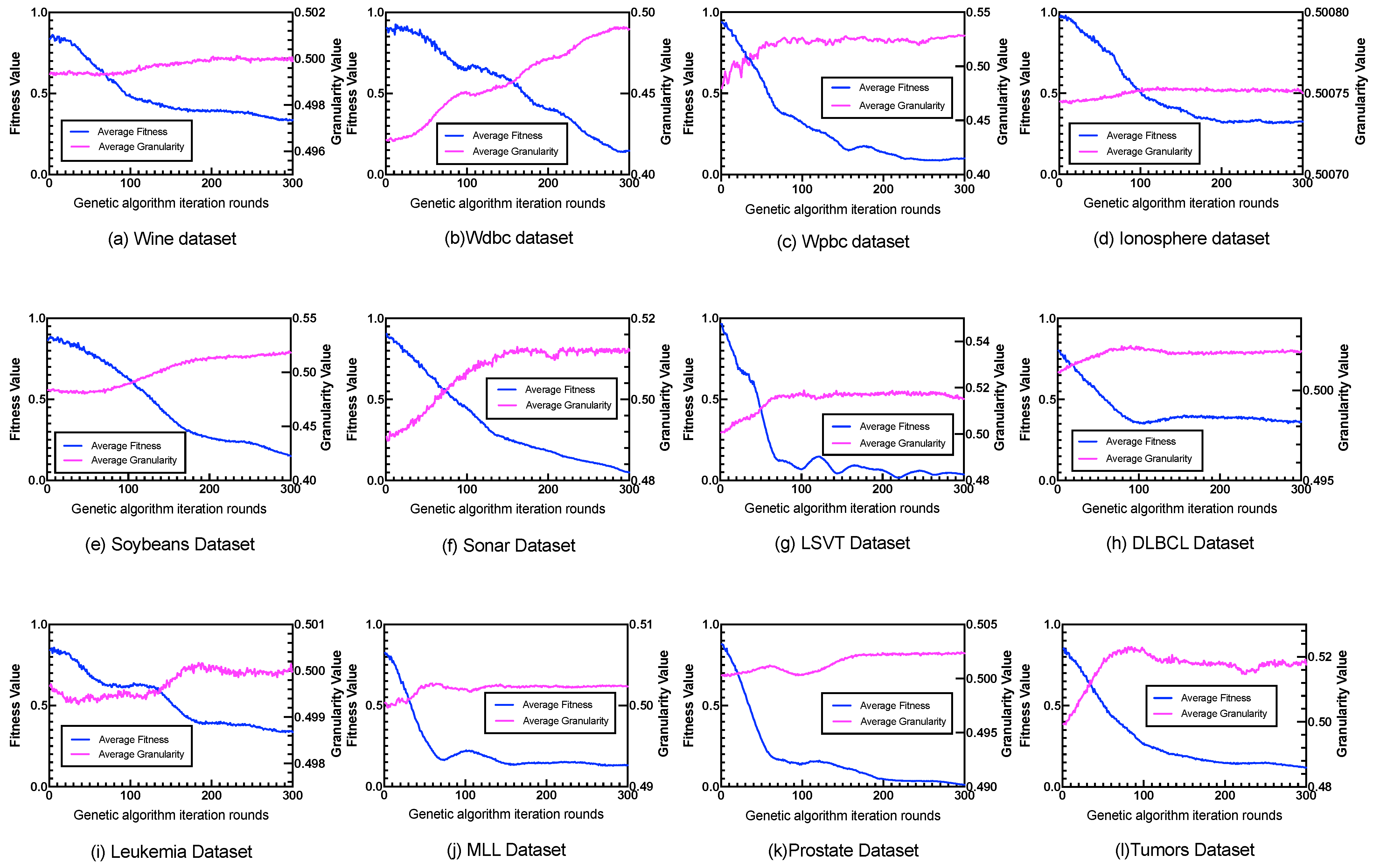
To verify the generalization ability of the GEK-NN model, it was applied to classify 12 additional datasets over 300 iterations, tracking the average fitness and granularity values per iteration. Since RMSE from the Elastic Net network plays a primary role in the fitness function, granularity variation is limited by parameter w g and changes only slightly. As shown in Figure 7, average granularity steadily increases and converges, indicating an optimal feature subset size. Even after granularity converges, the fitness function continues decreasing, showing that the algorithm optimizes for subsets with lower RMSE within similar granularity. Most datasets display stable granularity convergence, though Wdbc shows more fluctuations. It is worth noting that, among the datasets evaluated, the Wdbc dataset exhibits more apparent fluctuations in granularity convergence, contrasting with the stable behavior observed in other datasets. This instability can be attributed to the intrinsic structure of the Wdbc dataset, which contains 30 real-valued features derived from statistical descriptors (e.g., mean radius, standard deviation of texture, worst perimeter, etc.). These features are known to exhibit strong correlations and redundancy. Such internal structure leads to a scenario where multiple distinct feature subsets yield highly similar predictive performance under RMSE evaluation. As a result, the evolutionary search process in GEK-NN may encounter several quasi-optimal regions in the search space, causing the granularity to oscillate between similarly performing solutions rather than converging smoothly. This phenomenon reflects the presence of a flat or multi-modal fitness landscape, where the marginal differences between candidate subsets are not sufficiently distinct to drive consistent convergence. Despite the observed fluctuations, the final performance of GEK-NN on Wdbc remains strong, indicating that the algorithm is still capable of identifying competitive feature subsets, albeit through a more explorative search trajectory.
Datasets such as Wpbc, Sonar, LSVT, MLL, and Prostate have lower fitness values, indicating effective classification with smaller feature subsets.

4.4. Performance Evaluation

To better observe the effect of GEK-NN on different datasets, we classify all the mentioned datasets, Seeds, Wine, Wdpc, Wpbc, Ionosphere, Soybean, Sonar, and LSVT datasets as one class (Table 2), which is characterized by a large number of samples but a small number of feature counts, and the other class of datasets is the DLBCL, Leukemia, MLL, Prostate, and Tumors datasets (Table 3); this class is characterized by containing very few samples but a very large number of features, because these datasets are gene-related. The performance of the GEK-NN model can be analyzed more intuitively by analyzing the results of different kinds of datasets.
This part will introduce the parameter value output of the dataset during the algorithm as well as the result output, and it will also compare the results of different EK-NN algorithms; in the EK-NN algorithms, we choose the following types of algorithms for feature selection to compare with our own proposed algorithms:
(1)
Original EK-NN method.
(2)
Feature-selection methods based on Genetic Algorithms with embedded machine learning models (KNN, SVM, and logistic regression) applied to EK-NN models.
(3)
Feature-selection method using fuzzy mathematics and domain knowledge for EK-NN models [25,39,40,41]. The cited algorithms NDD, NMI, FINEN, and REK-NN all belong to a class of algorithms for feature selection, and in the paper [25] these algorithms are used for comparison by applying them to the EK-NN model.
All EK-NN-based comparison methods were implemented under a unified Genetic Algorithm (GA) framework to ensure experimental consistency. The core difference among these methods lies in the fitness evaluation model used to guide evolution, while all other GA configurations remained identical. For each technique, parameters were optimized using the same 10-fold cross-validation strategy repeated 10 times. The best-performing configuration on the training folds was selected for evaluation on the test fold. Distance-based models, such as NMI-, NDD-, and REK-NN-based variants, involve weighting parameters that were set according to the procedures described in their original papers and further adjusted to maximize classification accuracy within the shared evaluation pipeline. All models employed the Euclidean distance metric, and the preprocessing steps, data splits, and input formats were kept strictly consistent across all methods. This unified configuration ensures fair and unbiased comparisons among GEK-NN and the competing algorithms.
There are two main aspects of performance comparison, one is the accuracy of using the selected feature subset on the EK-NN model, and the other is the size of the feature subset of the different algorithms.
Accuracy evaluation. In Table 5, we observe that GEK-NN achieves strong performance across all UCI datasets, except for the Wine dataset, where its accuracy is slightly lower than that of REK-NN. This exception provides valuable insight into the limitations and potential extensions of GEK-NN. Both GEK-NN and REK-NN selected feature subsets of similar size on the Wine dataset, indicating comparable granularity preferences in feature selection. However, although the subset selected by REK-NN exhibits a higher RMSE than that of GEK-NN, it leads to superior classification accuracy when used in the EK-NN model. A deeper analysis suggests that this phenomenon is likely due to the inherent characteristics of the Wine dataset. It contains only 13 physicochemical features with well-defined semantic meanings and strong inter-feature correlations. In such low-dimensional yet semantically structured data, domain-informed relationships—such as those modeled by REK-NN—can play a crucial role in guiding the selection of synergistic features. RMSE, as a purely statistical fitting measure, may not adequately capture these subtle but semantically meaningful dependencies, which can lead to suboptimal feature subset choices in such contexts. This result reveals a potential limitation of the current GEK-NN framework: its reliance on data-driven objective functions without explicit incorporation of domain knowledge. To address this, future versions of GEK-NN could be extended to include feature relevance priors or structural information, such as correlation graphs or domain-annotated attributes, thereby enabling it to better adapt to datasets where domain concepts carry disproportionate weight relative to pure statistical fit.
In other models that also use the Genetic Algorithm framework, with the errors of the KNN, SVM, and LG models used as the fitness functions, the model performance varies across different datasets. Table 5 shows that GA-KNN, GA-SVM, and GA-LG obviously perform poorly on high-dimensional datasets due to these classifiers’ weaker ability to reduce irrelevant features, which results in poorer classification performance. However, on standard UCI datasets, these models show relatively better performance, highlighting their effectiveness in lower-dimensional scenarios.
For high-dimensional datasets, as shown in Table 6, the NDD, NMI, and FINEN methods perform well in feature selection for the DLBCL, Leukemia, and MLL datasets, achieving high accuracy, with RE-KNN demonstrating the best performance on the MLL dataset. However, the NDD, NMI, and FINEN methods perform poorly on the Prostate and Tumors datasets. The fundamental reason for this is the lack of global information in domain analysis for these datasets. In contrast, the genetic algorithm-based feature-selection approach can perform a comprehensive global analysis instead of analyzing only partial domain information. Using the GEK-NN method effectively converges the size of the feature subset and achieves better results, which is particularly crucial for high-dimensional gene datasets. As seen in Table 6, GEK-NN performs excellently on all datasets except for the MLL dataset, where its accuracy is slightly lower than that of RE-KNN.
The GEK-NN model exhibits significant performance advantages across both conventional UCI datasets and high-dimensional genomic datasets. On the UCI benchmarks, GEK-NN attains the highest classification accuracy on six out of seven datasets, achieving improvements of up to 12.91% over the original EK-NN algorithm (e.g., LSVT: from 81.20% to 94.11%). Furthermore, the model demonstrates consistently lower standard deviations compared to other approaches, indicating enhanced robustness and stability (e.g., Sonar: ±0.93 for GEK-NN versus ±3.18 for GA-SVM). In the context of genomic datasets, GEK-NN achieves substantial performance gains, with accuracy improvements exceeding 14% in certain cases (e.g., MLL: from 84.54% to 99.28%), while maintaining minimal variance (typically within ±0.5). These empirical results collectively underscore the efficacy of GEK-NN in delivering both accurate and stable classification outcomes, particularly under complex and high-dimensional feature conditions.
An evaluation of the size of the feature subsets. The Upsetplot tool is used to analyze feature subsets selected by different feature-selection algorithms for EKNN. This tool examines set relationships among feature subsets generated by various algorithms for each dataset. Each image includes eight feature subsets: the horizontal bar chart shows the number of features in each set, while the vertical bar chart represents intersections between different sets. Each dot signifies a set, and lines between dots indicate intersections (shared features).
As seen in Figure 8, UCI datasets show more intersections between feature sets selected by different algorithms, likely due to their lower dimensionality and correlated features. This often leads to higher overlap in important features selected, making it more crucial to reduce redundancy by selecting fewer features to lower algorithm complexity. Our proposed algorithm (set8) ranks high among all algorithms, containing fewer features.
In contrast, for high-dimensional gene datasets, weak correlations between gene features, high sparsity, and noise interference lead different algorithms to select distinct key features, resulting in minimal or no overlap between subsets. Our proposed algorithm performs well on high-dimensional gene datasets, selecting fewer features while maintaining high classification accuracy, demonstrating that GE-KNN effectively identifies sparse features and patterns.
In high-dimensional gene datasets, the number of elements in the feature subsets output by various feature-selection algorithms is generally larger than that in standard UCI datasets due to the sparsity of key information in gene data. The features in gene data (e.g., gene expression levels) often exhibit complex interactions and correlations. The function of certain genes may depend on the combined expression of multiple features rather than a single feature, which is why the retained feature subsets for high-dimensional gene datasets contain more elements. The intersection between the feature subsets output by different feature-selection algorithms is relatively small because gene expression is complex and interrelated, and different algorithms follow different principles for selecting features.

4.5. Limitations and Discussions on Model Complexity

While GEK-NN demonstrates strong performance across diverse datasets, several limitations remain that deserve attention. First, the convergence speed of the genetic search component can be relatively slow, particularly when applied to high-dimensional datasets such as genomic data containing tens of thousands of features. This is primarily due to the combinatorial nature of the feature space, which may require a large number of generations and evaluations to identify stable and compact feature subsets. Consequently, the computational overhead is higher compared to simpler filter-based or greedy methods. Future work may address this limitation by incorporating parallelized evolution strategies, adaptive population control, or hybrid meta-heuristics (e.g., memetic algorithms) to improve convergence efficiency without sacrificing performance. Second, GEK-NN involves several hyperparameters that can impact model performance, including crossover and mutation rates in the genetic algorithm, as well as the Elastic Net regularization coefficients. Although all hyperparameters in this study were tuned via cross-validation to ensure fairness and reliability, the model remains sensitive to suboptimal configurations. To address this, future versions may incorporate automated hyperparameter optimization techniques such as Bayesian search or reinforcement learning, which could enhance robustness and reduce reliance on manual tuning. In summary, despite its superior accuracy and robustness, GEK-NN still faces challenges in convergence efficiency and parameter sensitivity. Addressing these limitations will be key to improving the scalability and practicality of the model in large-scale or real-time applications.

5. Conclusions

In this paper, we propose a model, GEK-NN, that performs feature selection within the framework of Genetic Algorithms and classification within the framework of Evidence Theory. GEK-NN effectively reduces superfluous input features, thereby decreasing classification complexity. It employs Elastic Net to evaluate the performance of feature individuals while pruning irrelevant variables, and introduces the concept of granularity to quantify subset compactness. This enables the Genetic Algorithm to converge more efficiently to high-performing and compact feature subsets. Compared to the original EK-NN model, GEK-NN exhibits clear advantages on both conventional UCI datasets and high-dimensional gene expression data. Moreover, in contrast to traditional GA-based methods, the introduction of Elastic Net and granularity into the fitness evaluation enhances both the subset quality and classification accuracy.
Improving Generalizability and Methodological Scope. Further research will focus on extending the applicability of GEK-NN to more complex and realistic classification scenarios. For example, in datasets containing overlapping or noisy feature regions, we plan to refine the fitness function by incorporating region-specific penalty parameters to better capture feature ambiguity. Additionally, to address the computational challenges posed by ultra-high-dimensional data, we intend to parallelize the granularity-based search process using distributed computing platforms such as Apache Spark or Dask, enabling scalable and efficient evaluation of feature populations. While this study centers on feature selection specifically for the EK-NN framework, we recognize the importance of general-purpose feature-selection techniques in the broader machine learning community. In future work, we plan to extend our approach by comparing it with more widely adopted and generalized feature-selection methods. These comparative studies will help assess the transferability and effectiveness of our algorithm beyond EK-NN and enable fairer benchmarking across diverse model families.
Expanding Real-World Application Scenarios. We envision that the GEK-NN model holds significant potential for real-world applications where high-dimensional data presents major challenges. In precision healthcare, GEK-NN could assist in gene-based disease classification or biomarker selection by identifying compact, informative feature subsets. In finance, its robust feature-reduction mechanism may improve both transparency and performance in tasks such as fraud detection and credit risk assessment. In large-scale IoT systems, GEK-NN can serve as an offline pre-processing tool to eliminate redundancy before inference. Finally, we plan to develop a lightweight software toolkit based on GEK-NN, facilitating its adoption in genomics, IoT, and other data-intensive domains.

Author Contributions

Conceptualization, Y.L. and Y.Z.; Methodology, Y.L.; Software, Y.L.; Validation, Y.L. and Y.Z.; Validation, Y.L. and X.W.; Formal analysis, Y.L.; Writing—original draft, Y.L.; Writing—review &editing, Y.Z., X.W. and X.Q.; Visualization, Y.L. and X.Q.; Supervision, Y.Z. All authors reviewed the manuscript. All authors have read and agreed to the published version of the manuscript.

Funding

This work was supported by the National Key R&D Program of China under Grant 2021YFC3300205 and the R&D Project for a Comprehensive Urban Safety Risk Monitoring and Early Warning Platform Based on Typical Scenario Model Algorithms, with the project number Y915230FHD0007.

Data Availability Statement

Data is provided within the manuscript.

Conflicts of Interest

Xudong Wang is employed by the company Unicom Digital Technology Co., Ltd. The remaining authors declare that the research was conducted in the absence of any commercial or financial relationships that could be construed as a potential conflict of interest.

References

  1. Cover, T.; Hart, P. Nearest neighbor pattern classification. IEEE Trans. Inf. Theory 1967, 13, 21–27. [Google Scholar] [CrossRef]
  2. Denoeux, T. A k-nearest neighbor classification rule based on Dempster-Shafer theory. IEEE Trans. Syst. Man, Cybern. 1995, 25, 804–813. [Google Scholar] [CrossRef]
  3. Dempster, A.P. Upper and Lower Probabilities Induced by a Multivalued Mapping; Springer: Berlin/Heidelberg, Germany, 2008; pp. 57–72. [Google Scholar]
  4. Denœux, T. 40 years of Dempster-Shafer theory. Int. J. Approx. Reason. 2016, 79, 1–6. [Google Scholar] [CrossRef]
  5. Shafer, G. A Mathematical Theory of Evidence; Princeton University Press: Princeton, NJ, USA, 1976; Volume 42. [Google Scholar]
  6. Kanjanatarakul, O.; Kuson, S.; Denoeux, T. An evidential K-nearest neighbor classifier based on contextual discounting and likelihood maximization. In Belief Functions: Theory and Applications, Proceedings of the 5th International Conference (BELIEF 2018), Compiègne, France, 17–21 September 2018; Proceedings 5; Springer: Cham, Switzerland, 2018; pp. 155–162. [Google Scholar]
  7. Huang, L.; Fan, J.; Zhao, W.; You, Y. A new multi-source transfer learning method based on two-stage weighted fusion. Knowl.-Based Syst. 2023, 262, 110233. [Google Scholar] [CrossRef]
  8. Toman, P.; Ravishanker, N.; Rajasekaran, S.; Lally, N. Online Evidential Nearest Neighbour Classification for Internet of Things Time Series. Int. Stat. Rev. 2023, 91, 395–426. [Google Scholar] [CrossRef]
  9. Trabelsi, A.; Elouedi, Z.; Lefevre, E. An ensemble classifier through rough set reducts for handling data with evidential attributes. Inf. Sci. 2023, 635, 414–429. [Google Scholar] [CrossRef]
  10. Zouhal, L.M.; Denoeux, T. An evidence-theoretic k-NN rule with parameter optimization. IEEE Trans. Syst. Man Cybern. Part C (Appl. Rev.) 1998, 28, 263–271. [Google Scholar] [CrossRef]
  11. Su, Z.-G.; Wang, P.-H.; Yu, X.-J. Immune genetic algorithm-based adaptive evidential model for estimating unmeasured parameter: Estimating levels of coal powder filling in ball mill. Expert Syst. Appl. 2010, 37, 5246–5258. [Google Scholar] [CrossRef]
  12. Gong, C.-Y.; Su, Z.-G.; Zhang, X.-Y.; Yang, Y. Adaptive evidential K-NN classification: Integrating neighborhood search and feature weighting. Inf. Sci. 2023, 648, 119620. [Google Scholar] [CrossRef]
  13. Liu, Z.-G.; Pan, Q.; Dezert, J.; Mercier, G. Hybrid classification system for uncertain data. IEEE Trans. Syst. Man, Cybern. Syst. 2016, 47, 2783–2790. [Google Scholar] [CrossRef]
  14. Gong, C.; Su, Z.-G.; Wang, P.-H.; Wang, Q.; You, Y. Evidential instance selection for K-nearest neighbor classification of big data. Int. J. Approx. Reason. 2021, 138, 123–144. [Google Scholar] [CrossRef]
  15. Altınçay, H. Ensembling evidential k-nearest neighbor classifiers through multi-modal perturbation. Appl. Soft Comput. 2007, 7, 1072–1083. [Google Scholar] [CrossRef]
  16. Trabelsi, A.; Elouedi, Z.; Lefevre, E. Ensemble enhanced evidential k-NN classifier through random subspaces. In Symbolic and Quantitative Approaches to Reasoning with Uncertainty, Proceedings of the 14th European Conference (ECSQARU 2017), Lugano, Switzerland, 10–14 July 2017; Springer: Cham, Switzerland, 2017; pp. 212–221. [Google Scholar]
  17. Denoeux, T.; Kanjanatarakul, O.; Sriboonchitta, S. A new evidential k-nearest neighbor rule based on contextual discounting with partially supervised learning. Int. J. Approx. Reason. 2019, 113, 287–302. [Google Scholar] [CrossRef]
  18. Vommi, A.M.; Battula, T.K. A hybrid filter-wrapper feature selection using Fuzzy KNN based on Bonferroni mean for medical datasets classification: A COVID-19 case study. Expert Syst. Appl. 2023, 218, 119612. [Google Scholar] [CrossRef]
  19. Zhang, X.; Xiao, H.; Gao, R.; Zhang, H.; Wang, Y. K-nearest neighbors rule combining prototype selection and local feature weighting for classification. Knowl.-Based Syst. 2022, 243, 108451. [Google Scholar] [CrossRef]
  20. Guyon, I.; Elisseeff, A. An introduction to variable and feature selection. J. Mach. Learn. Res. 2003, 3, 1157–1182. [Google Scholar]
  21. Li, Y.; Chen, C.-Y.; Wasserman, W.W. Deep feature selection: Theory and application to identify enhancers and promoters. J. Comput. Biol. 2016, 23, 322–336. [Google Scholar] [CrossRef]
  22. Molchanov, D.; Ashukha, A.; Vetrov, D. Variational dropout sparsifies deep neural networks. In Proceedings of the 34th International Conference on Machine Learning (ICML), Sydney, Australia, 6–11 August 2017; pp. 2498–2507. [Google Scholar]
  23. Gaudel, R.; Sebag, M. Feature selection as a one-player game. In Proceedings of the 27th International Conference on Machine Learning (ICML), Haifa, Israel, 21–24 June 2010; pp. 359–366. [Google Scholar]
  24. Lian, C.; Ruan, S.; Denœux, T. An evidential classifier based on feature selection and two-step classification strategy. Pattern Recognit. 2015, 48, 2318–2327. [Google Scholar] [CrossRef]
  25. Su, Z.-G.; Hu, Q.; Denoeux, T. A distributed rough evidential K-NN classifier: Integrating feature reduction and classification. IEEE Trans. Fuzzy Syst. 2020, 29, 2322–2335. [Google Scholar] [CrossRef]
  26. Holland, J.H. Adaptation in Natural and Artificial Systems: An Introductory Analysis with Applications to Biology, Control, and Artificial Intelligence; MIT Press: Cambridge, MA, USA, 1992. [Google Scholar]
  27. Katoch, S.; Chauhan, S.S.; Kumar, V. A review on genetic algorithm: Past, present, and future. Multimed. Tools Appl. 2021, 80, 8091–8126. [Google Scholar] [CrossRef]
  28. Jiao, R.; Nguyen, B.H.; Xue, B.; Zhang, M. A survey on evolutionary multiobjective feature selection in classification: Approaches, applications, and challenges. IEEE Trans. Evol. Comput. 2023, 28, 1156–1176. [Google Scholar] [CrossRef]
  29. Oh, I.-S.; Lee, J.-S.; Moon, B.-R. Hybrid genetic algorithms for feature selection. IEEE Trans. Pattern Anal. Mach. Intell. 2004, 26, 1424–1437. [Google Scholar] [CrossRef]
  30. Fukushima, A.; Sugimoto, M.; Hiwa, S.; Hiroyasu, T. Elastic net-based prediction of IFN-β treatment response of patients with multiple sclerosis using time series microarray gene expression profiles. Sci. Rep. 2019, 9, 1822. [Google Scholar] [CrossRef]
  31. Park, I.W.; Mazer, S.J. Overlooked climate parameters best predict flowering onset: Assessing phenological models using the elastic net. Glob. Change Biol. 2018, 24, 5972–5984. [Google Scholar] [CrossRef]
  32. Zou, H.; Hastie, T. Regularization and variable selection via the elastic net. J. R. Stat. Soc. Ser. Stat. Methodol. 2005, 67, 301–320. [Google Scholar] [CrossRef]
  33. Amini, F.; Hu, G. A two-layer feature selection method using genetic algorithm and elastic net. Expert Syst. Appl. 2021, 166, 114072. [Google Scholar] [CrossRef]
  34. Zhang, Z.; Lai, Z.; Xu, Y.; Shao, L.; Wu, J.; Xie, G.-S. Discriminative elastic-net regularized linear regression. IEEE Trans. Image Process. 2017, 26, 1466–1481. [Google Scholar] [CrossRef]
  35. Dong, H.; Li, T.; Ding, R.; Sun, J. A novel hybrid genetic algorithm with granular information for feature selection and optimization. Appl. Soft Comput. 2018, 65, 33–46. [Google Scholar] [CrossRef]
  36. Blake, C.L.; Merz, C.J. UCI Repository of Machine Learning. 1998. Available online: http://www.ics.uci.edu/mlearn/MLRepository (accessed on 1 January 2024).
  37. Kent Ridge Bio-Medical Dataset. 2015. Available online: http://datam.i2r.atar.edu.sg/datasets/krbd/index.html (accessed on 1 January 2024).
  38. Derrac, J.; Garcia, S.; Sanchez, L.; Herrera, F. Keel data-mining software tool: Data set repository, integration of algorithms and experimental analysis framework. J.-Mult.-Valued Log. Soft Comput. 2015, 17, 255–287. [Google Scholar]
  39. Hu, Q.; Yu, D.; Liu, J.; Wu, C. Neighborhood rough set based heterogeneous feature subset selection. Inf. Sci. 2008, 178, 3577–3594. [Google Scholar] [CrossRef]
  40. Hu, Q.; Zhang, L.; Zhang, D.; Pan, W.; An, S.; Pedrycz, W. Measuring relevance between discrete and continuous features based on neighborhood mutual information. Expert Syst. Appl. 2011, 38, 10737–10750. [Google Scholar] [CrossRef]
  41. Hu, Q.; Yu, D.; Xie, Z.; Liu, J. Fuzzy probabilistic approximation spaces and their information measures. IEEE Trans. Fuzzy Syst. 2006, 14, 191–201. [Google Scholar] [CrossRef]
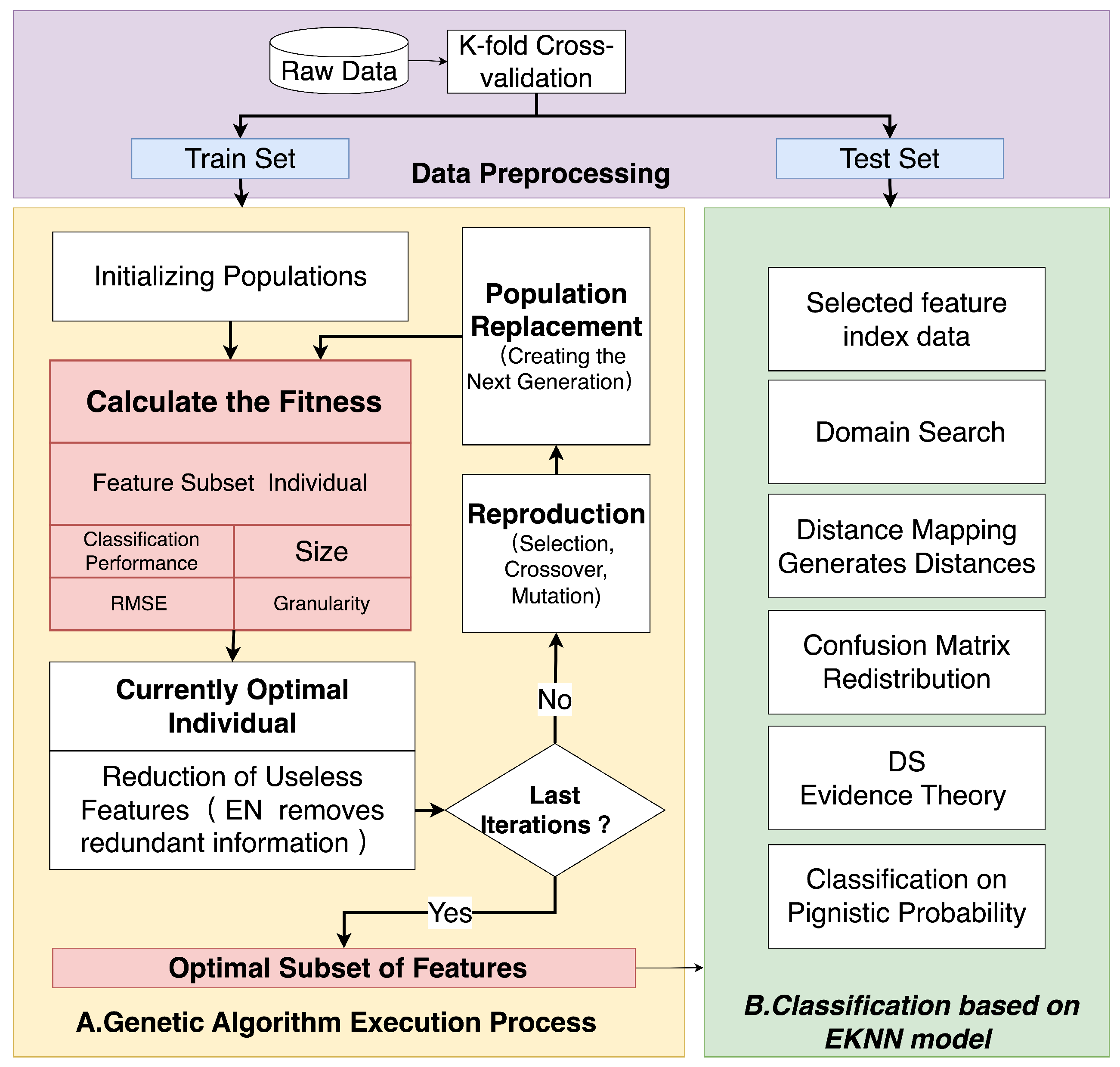
Figure 1. GEK-NN implementation process.
Bdcc 09 00202 g001
Figure 2. The variation in parameter values related to the Seeds dataset during the feature-selection process.
Bdcc 09 00202 g002
Figure 3. The average RMSE of individuals with different numbers of features in the iteration round.
Bdcc 09 00202 g003
Figure 4. Iterative details of average RMSE values for individuals with different number of features.
Bdcc 09 00202 g004
Figure 5. The Seeds dataset correctly distinguished by EK-NN for the test samples (compared to KNN). Each subgraph (af) represents the neighbor distribution of different test samples.
Bdcc 09 00202 g005
Figure 6. Sensitivity of GEK-NN performance to w g on Wine and DLBCL datasets. A balance between accuracy and granularity is observed around w g = 0.15 .
Bdcc 09 00202 g006
Figure 7. The convergence of the proposed genetic algorithm-based feature selection algorithm across all datasets.
Bdcc 09 00202 g007
Figure 8. The relationship diagram of feature sets selected by different algorithms is visualized using Upsetplot (Set 1–8 correspond to algorithms NDD-based EK-NN, NMI-based EK-NN, FINEN-based EK-NN, REK-NN, GA-KNN-based EK-NN, GA-SVM-based EK-NN, GA-LG-based EK-NN, and GEK-NN, respectively).
Bdcc 09 00202 g008
Table 1. Parameters used in the Genetic Algorithm framework.
Parameter NameParameter SettingSpecific Value
Population size P size Determines how many chromosomes will initialize50
Chromosome length H size The number of genes contained in the chromosomeequal to the number of features
Crossover modeThe mode of crossover of the chromosomeSingle point (crossover at one site only)
Probability of mutation P m Probability of chromosome mutation0.05
Number of iterations TTotal number of iterations performed300
Table 2. UCI datasets.
IDDatasetSamplesAttributesClasses
1Seeds21073
2Wine178133
3Wdbc569302
4Wpbc198332
5Ionosphere351342
6Soybean47354
7Sonar208602
8LSVT1263092
Table 3. High-dimensional gene datasets.
IDDatasetSamplesAttributesClasses
9DLBCL7754692
10Leukemia7211,2253
11MLL7211,2253
12Prostate13612,6002
13Tumors32712,5887
Table 4. Performance of GEK-NN under varying w g values on Wine and DLBCL datasets. Higher granularity implies a more compact feature subset. The best results are highlighted in bold.
w g WineDLBCL
Accuracy (%) Granularity Accuracy (%) Granularity
0.0594.30.6597.20.48
0.1095.60.5496.30.35
0.1598.50.4899.10.38
0.2096.10.4598.90.37
0.2595.00.4998.20.28
0.3093.70.3996.50.22
0.3591.20.3094.10.20
0.4089.60.2691.70.19
0.4587.50.2289.30.17
0.5086.10.2086.90.15
Table 5. Average accuracy of algorithms based on the GEK-NN model and eight other models (for the UCI datasets).
DatasetsOriginal EK-NNNDD Based EK-NNNMI Based EK-NNFINEN Based EK-NNREK-NNGA-KNN Based EK-NNGA-SVM Based EK-NNGA-LG Based EK-NNGEK-NN
Wine 97.94 ± 1.12 98.14 ± 0.95 98.43 ± 0.78 97.93 ± 0.84 98.96 ± 0.55 96.14 ± 1.31 92.73 ± 2.17 95.91 ± 1.05 98.45 ± 0.68
Wdbc 96.55 ± 0.96 96.80 ± 0.83 96.82 ± 0.81 96.45 ± 0.74 97.21 ± 0.59 95.61 ± 1.02 96.05 ± 0.87 96.78 ± 0.85 97.36 ± 0.51
Wpbc 74.09 ± 2.54 79.12 ± 2.03 77.94 ± 1.84 77.89 ± 2.16 81.93 ± 1.25 81.24 ± 1.58 81.75 ± 1.34 78.77 ± 1.77 82.50 ± 1.01
Ion. 89.54 ± 1.67 92.11 ± 1.10 91.82 ± 0.95 90.59 ± 1.03 93.31 ± 0.84 85.17 ± 2.05 90.21 ± 1.52 89.43 ± 1.44 94.32 ± 0.72
Soybean 99.67 ± 0.31 100.00 ± 0.00 100.00 ± 0.00 100.00 ± 0.00 100.00 ± 0.00 97.65 ± 0.44 98.79 ± 0.39 98.96 ± 0.42 100.00 ± 0.00
Sonar 80.24 ± 2.78 82.07 ± 2.01 83.96 ± 1.66 82.47 ± 1.85 89.88 ± 1.07 87.30 ± 1.14 79.76 ± 3.18 82.14 ± 2.41 90.87 ± 0.93
LSVT 81.20 ± 3.03 87.69 ± 2.71 90.77 ± 2.12 87.92 ± 2.30 90.85 ± 1.76 80.39 ± 3.19 82.35 ± 2.76 88.43 ± 2.02 94.11 ± 1.01
“Ion.” is the abbreviation of “Ionosphere”.
Table 6. Average accuracy of algorithms based on the GEK-NN model and eight other models (for the high-dimensional gene datasets).
DatasetsOriginal EK-NNNDD Based EK-NNNMI Based EK-NNFINEN Based EK-NNREK-NNGA-KNN Based EK-NNGA-SVM Based EK-NNGA-LG Based EK-NNGEK-NN
DLBCL 86.03 ± 3.15 98.96 ± 0.58 99.48 ± 0.41 99.21 ± 0.47 98.27 ± 0.68 86.53 ± 2.71 86.23 ± 2.40 85.05 ± 2.96 99.16 ± 0.36
Leu. 86.54 ± 2.78 96.21 ± 0.74 97.27 ± 0.61 96.66 ± 0.65 99.50 ± 0.35 89.17 ± 2.03 90.27 ± 1.89 88.61 ± 2.28 98.35 ± 0.39
MLL 84.54 ± 3.25 97.16 ± 0.69 96.41 ± 0.77 96.91 ± 0.66 99.14 ± 0.32 88.18 ± 1.95 86.55 ± 2.09 90.57 ± 1.76 99.28 ± 0.28
Prostate 78.88 ± 3.54 87.27 ± 1.94 93.32 ± 1.22 88.12 ± 1.87 97.68 ± 0.41 84.13 ± 2.33 86.89 ± 1.76 89.93 ± 1.69 98.23 ± 0.46
Tumors 82.49 ± 2.61 81.93 ± 2.45 86.45 ± 2.03 82.95 ± 2.51 93.60 ± 0.92 83.62 ± 2.17 85.19 ± 1.92 82.74 ± 2.39 94.67 ± 0.58
“Leu.” is the abbreviation of “Leukemia”.
Disclaimer/Publisher’s Note: The statements, opinions and data contained in all publications are solely those of the individual author(s) and contributor(s) and not of MDPI and/or the editor(s). MDPI and/or the editor(s) disclaim responsibility for any injury to people or property resulting from any ideas, methods, instructions or products referred to in the content.