Abstract
College enrollment has long been recognized as a critical pathway to better employment prospects and improved economic outcomes. However, the overall enrollment rates have declined in recent years, and students with a lower socioeconomic status (SES) or those from disadvantaged backgrounds remain significantly underrepresented in higher education. To investigate the factors influencing college enrollment among low-SES high school students, this study analyzed data from the High School Longitudinal Study of 2009 (HSLS:09) using five widely used machine learning algorithms. The sample included 5223 ninth-grade students from lower socioeconomic backgrounds (51% female; Mage = 14.59) whose biological parents or stepparents completed a parental questionnaire. The results showed that, among all five classifiers, the random forest algorithm achieved the highest classification accuracy at 67.73%. Additionally, the top three predictors of enrollment in 2-year or 4-year colleges were students’ overall high school GPA, parental educational expectations, and the number of close friends planning to attend a 4-year college. Conversely, the most important predictors of non-enrollment were high school GPA, parental educational expectations, and the number of close friends who had dropped out of high school. These findings advance our understanding of the factors shaping college enrollment for low-SES students and highlight two important factors for intervention: improving students’ academic performance and fostering future-oriented goals among their peers and parents.
1. Introduction
Educational attainment is strongly associated with improved employment outcomes, higher income levels, and greater overall well-being. To better understand the factors that influence college enrollment, prior research has examined a range of contributors, including student characteristics (e.g., academic ability, school engagement, and motivation [1,2,3]), parent and family factors (e.g., parental expectations, involvement, and college savings [4,5,6]), peer influences (e.g., friends’ college plans and communication about school [7,8]), and school-level characteristics (e.g., school environment and counselor contact [9,10]). However, many of these studies were limited by computational constraints, often examining only a small subset of factors rather than taking a comprehensive, theory-driven approach. Moreover, relatively few studies have focused specifically on high school students from low-SES backgrounds, who are among the least likely to pursue higher education [11]. To address these gaps, the present study aimed to identify the ten most influential predictors of college enrollment among low-SES high school students, grounded in ecological systems theory. Furthermore, this study applied explainable machine-learning techniques to reveal how these factors shape enrollment outcomes. The findings from this study could provide actionable insights for educational practitioners to enhance low-SES high school students’ college enrollment, which would be beneficial for their future employment and development.
2. Related Work
This section reviews the literature on the current state of college enrollment, the key factors influencing college enrollment decisions, and the theoretical framework that can be used to organize these factors, and it provides an introduction of explainable artificial intelligence techniques. Building on this review, this section further identifies gaps in the existing research and presents the research questions that this study aims to address.
2.1. College Enrollment
College enrollment has long been recognized as a critical determinant of economic outcomes, consistently linked to better employment prospects and higher earnings [12]. Data from the U.S. Bureau of Labor Statistics highlighted profound educational disparities in unemployment rates: workers without a high school diploma face unemployment rates three to four times higher than those with a bachelor’s degree or higher. This disparity was especially pronounced during the COVID-19 pandemic, when the average unemployment rate for bachelor’s degree holders was approximately 8%, but 17% for high school graduates who had not enrolled in any college [13,14]. Furthermore, the level of educational attainment is strongly associated with income. In 2020, the median American household income for those maintained by someone with at least a bachelor’s degree was USD 106,936, compared to USD 63,653 for those with some college education and USD 47,405 for high school graduates [15]. By 2023, these income gaps remained substantial: USD 126,800 for bachelor’s degree holders, USD 73,610 for those with some college, USD 55,810 for high school graduates, and USD 36,620 for individuals without a high school diploma [16].
Despite the well-documented benefits of college enrollment, enrollment rates have steadily declined since 2010. According to the National Center for Education Statistics (NCES), college enrollment increased by over 20% between 2000 and 2010, peaking in the fall of 2010, but has consistently declined in the years since 2010 [17]. Undergraduate enrollment dropped by 2.5% from fall 2019 to fall 2020, followed by another 2.7% decline in fall 2021 [18]. By 2024, the decline had reached 5%, signaling a concerning downward trend. Furthermore, from an educational equity standpoint, this declining trend has a greater impact on low-SES students than on high-SES students. Based on the report from the National Student Clearinghouse, the proportion of high school graduates at high-poverty high schools that enrolled in college declined by 32.6% in 2020, compared with a 16.4% decline for those in low-poverty schools [18]. These patterns underscore the urgent need to examine the factors influencing college enrollment among low-SES students, in order to identify actionable interventions that can help mitigate these disparities.
2.2. Factors Affecting College Enrollment
Numerous studies have explored the predictors of high school students’ college enrollment from various perspectives. Students’ personal characteristics have been one of the most frequently examined factors. For example, using longitudinal data from the Educational Longitudinal Study of 2002, Bates and Anderson [1] revealed that students’ high school grade point average (GPA) and students’ expectations for future educational attainment significantly predict students’ probability of post-secondary enrollment. Students’ school engagement [3], motivation [19], and sense of belonging [20] in their high school were also important factors for predicting college enrollment. Another aspect that drew researchers’ attention was the strong influence of peer networks on students’ college destinations [21,22]. For example, previous studies have explored the role of the number of the student’s friends planning on attending either 2- or 4-year colleges [10]. They found that, as the number of one’s friends attending a 4-year college increased, students were more likely to attend a 4-year institution. Friends’ college plans had a stronger impact on low-income students’ 4-year college enrollment than they did for a comparison sample of all U.S. high school graduates [8]. Parallel-process latent growth curve modeling revealed that steep increases in school-related communication with friends independently predicted college enrollment, consistently across racial/ethnic and parental education groups [7]. Furthermore, there has been some research examining the influence of parents and families on college enrollment. High school students whose parents were more involved in their lives and studies [23] and had greater educational expectations [5,6] were more likely to enroll in college. These two factors were particularly crucial for low-SES students to enroll in a 4-year college [24,25]. In addition, some studies have examined the role of school characteristics (e.g., teachers, counselors, administrators, and school climate). Previous studies have revealed that counselors and counseling programs [9,26], teacher expectations [27], and a positive school climate [28] benefit college enrollment as well. The last important factor was the policies of universities and governments on the provision of financial aid to students [29], but its significance has been questioned by some studies [30].
Although there are many potential predictors, earlier research only included one or a few due to computing constraints. However, with the increasing use of machine learning in education, some studies have attempted to predict college enrolment by including various factors simultaneously [31,32,33,34]. For example, Yang et al. [33] forecasted the number of freshman enrollments in Guangzhou province (China) before their registration. Their results showed that the backpropagation (BP) neural network outperformed the decision tree and random forest, with a 62.07% accuracy. In addition, Slim et al. [32] projected student enrolment at the University of New Mexico based on random forest and support vector machine algorithms to aid colleges in identifying characteristics that could maximize the prediction of students with a higher tendency to enroll at their institutions. They considered both student and college characteristics as predictors, such as the students’ gender, ethnicity, SAT score, GPA, parents’ income, institutional money, and financial aid offered by the school. The results indicated that support vector machines (SVMs) were superior to logistic regression, with an accuracy of 91.25%, and the identified factors included the amount of scholarships, the time of the admission decision, the GPA, and the student’s residency status.
2.3. Ecological Systems Theory
As mentioned above, numerous factors could influence students’ college enrollment, including students’ characteristics, parental and family characteristics, peers’ characteristics, schools’ characteristics, and the policies of universities and governments. All of these potential factors can be framed in Bronfenbrenner’s ecological systems theory [35]. Ecological systems theory views individual development as a complex system of relationships affected by multiple levels of the surrounding environment, from immediate settings of family and school to broad cultural values, laws, and customs. As shown in Figure 1, it identifies six interrelated systems that influence individual development. At the center is the individual and their personal characteristics, such as sex, age, health, and GPA (represented by the purple circle). Surrounding the individual is the microsystem (yellow circle), which includes institutions and groups that have the most immediate and direct impact on an individual’s development, such as family, school, and peers. The third system is the mesosystem (blue circle), which captures the interconnections among these microsystems, such as parent–teacher communication. The curved arrows within the circle represent these interconnections, while the bidirectional colored arrows highlight the reciprocal nature of influences across systems. The fourth system is the exosystem (light blue circle), encompassing social settings that indirectly affect the individual, such as parental workplace conditions. The fifth system is the macrosystem (dark blue circle), which refers to broader cultural and societal contexts, including values, norms, and ideologies. Finally, the chronosystem (green base) represents the dimension of time—encompassing life transitions and sociohistorical events that shape development over time. The vertical blue double-headed arrow between the chronosystem and time underscores the dynamic interaction between an individual’s age and historical context, emphasizing that the timing of life events can shape developmental outcomes: [36]. Among these systems, factors from individuals, microsystems, and interactions between microsystems (e.g., parent–school interactions) are often viewed as having the greatest impact on an individual’s development [37]. Therefore, ecological systems theory provides a valuable theoretical foundation for identifying factors that influence college enrollment, encompassing individual characteristics as well as influences from parents, peers, teachers, school counselors, administrators, and broader school contexts.
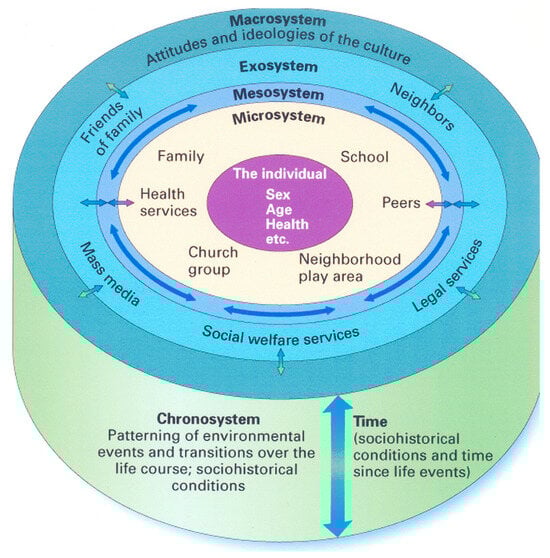
Figure 1.
Ecological systems theory.
2.4. Explainable Artificial Intelligence Techniques
While prior studies have employed machine learning to identify influential factors in college enrollment, few have focused on the explainability of their findings. However, in the social sciences, understanding how and why certain factors influence outcomes is essential. To bridge this gap, the field of computer science has developed explainable artificial intelligence (XAI), a subfield focused on generating human-interpretable explanations for AI systems’ decisions, behaviors, strengths, and limitations [38,39]. The rise of XAI stems from the widespread adoption of advanced AI techniques such as deep learning that do not provide an explanation for their results [39,40,41]. While these models offer a high predictive accuracy, their lack of transparency can lead to misleading interpretations, especially in high-stakes domains like healthcare and education. Without explainability, practitioners (e.g., policymakers or educators) may struggle to derive actionable insights from AI-driven findings [42].
Various XAI approaches have been proposed in recent years. A recent systematic review conducted by Minh et al. [43] categorized these approaches into three main types: pre-modeling explainability, interpretable models, and post-modeling explainability. Specifically, pre-modeling explainability focuses on data-centric techniques (e.g., exploratory analysis, statistical summarization, and feature transformation) to enhance the understanding of the dataset before model training. The interpretable models involve using inherently transparent algorithms (e.g., linear models, decision trees, and rule-based systems) whose internal logic and decision boundaries permit direct human examination. The most extensively developed category, post-modeling explainability, addresses model opacity through four types of techniques. First, textual justification generates natural language explanations of model decisions. Second, visual explanation employs tools such as layer-wise relevance propagation (LRP) heatmaps and local interpretable model-agnostic explanations (LIME) to create graphical interpretations of model behavior. Advanced methods include activation maximization for neural networks and decision path visualization for tree ensembles. Third, model simplification develops surrogate systems through rule extraction and prototype selection, preserving the predictive accuracy while enhancing the interpretability. Fourth, a feature relevance analysis quantifies variable importance through game-theoretic and statistical methods. SHAP (Shapley additive explanations) values provide theoretically-grounded feature attributions, whereas permutation importance and partial dependence plots reveal global relationships. Recent extensions enable temporal and interaction effect analyses for dynamic educational datasets. Among these, visualization, simplification, and feature relevance methods are three commonly used XAI methods, emphasizing their role in rendering AI systems more transparent and understandable [43].
2.5. The Present Study
Previous studies have explored the predictors of college enrollment from a diverse range of perspectives, and some of them have applied machine learning methods. However, there are still gaps in the current research. First, most of the previous studies have forecasted college enrollment numbers or rates from a school administration perspective to aid college admissions, which has led to a greater emphasis on the prediction accuracy of the model rather than on the reasons or variables that contribute to this higher accuracy. Nevertheless, identifying characteristics is particularly useful for researchers and practitioners, as they may determine which factors among a huge number are crucial for enhancing college enrollment. Second, although several studies have attempted to identify significant predictors, most of those predictors are not easily modifiable by students, teachers, administrators, or other stakeholders (i.e., non-actionable predictors), making it difficult to tailor interventions or adjust the current situation, system, or organization to promote college enrollment [44]. Finally, no study has used machine learning to systematically identify the predictors of low-SES students’ college enrollment. To address these gaps, this study aimed to investigate the ten most influential factors predicting college enrollment among low-SES high school students, grounded in ecological systems theory. Furthermore, this study employed XAI techniques to reveal how these factors influence enrollment outcomes. To our knowledge, this is the first study that used machine learning approaches to systematically identify and interpret key determinants of college enrollment specifically for low-SES high school student populations.
3. Methodology
This section outlines the data sources used in this study, the measurement of predictors and outcomes, the procedures for data pre-processing, and the methods for building and testing machine learning models. Additionally, this section details the evaluation metrics employed to assess the performance of the machine learning models and discusses the rationale behind the selection of specific algorithms for this study.
3.1. Participants and Procedure
This study sampled data from the High School Longitudinal Study of 2009 (HSLS:09), which is a nationally representative longitudinal study conducted by the National Center for Educational Statistics of the United States. The data are publicly available at the official website https://nces.ed.gov/surveys/hsls09/ (accessed on 10 April 2025). The HSLS:09 investigated 23,503 9th-graders from 944 schools in 2009, with the first follow-up in 2012 (12th grade), a 2013 update, and the second follow-up in 2016. In addition, data were also collected from the students’ parents, math and science teachers, school administrators, and school counselors. The current study focused exclusively on 7139 students from lower socioeconomic backgrounds (i.e., students who ranked 1 or 2 on the SES quintile composite score). After excluding students whose parental questionnaires were not from their biological parents or stepparents, the final sample size of this study was 5223 (51% female; Mage = 14.59, range: 13–17).
3.2. Measures
3.2.1. Dependent Variable
The dependent (i.e., response or target) variable of this study was the post-secondary enrollment level in 2016, with five response levels (0 = not enrolled, 1 = enrolled in a 4-year institution, 2 = enrolled in a 2-year institution, 3 = enrolled in a less-than-2-year institution, and 4 = enrolled, but institutional level unknown). This study re-coded students who chose 4 as missing values, since it was unable to determine at which college level they were enrolled. Moreover, in accordance with the common categories of college enrollment status of the National Center for Education Statistics [45] and taking into account the small sample size (n < 50) in category 3, we consolidated categories 2 and 3 and re-coded the response category into three levels (0 = not enrolled, 1 = enrolled in a 2-year or less institution, and 2 = enrolled in a 4-year institution).
3.2.2. Predictors
According to the ecological systems theory, the original 100 predictors of the current study were derived from four distinct sources, including student characteristics (e.g., overall high school GPA, expectations and aspirations for educational attainment, sense of school belonging, school engagement, school motivation, talking with significant others about going to college, and plans and preparations for the future), parental characteristics (e.g., parental expectations and aspirations for the student’s future educational attainment, parental involvement, and parental activities for helping the student’s preparation for life after high school), peers’ characteristics (e.g., close friends’ plans to attend college, close friends’ high school enrollment status, and their grades), and school characteristics (e.g., teachers’ expectations for students, school problems, school climate, school counseling programs, and school policies and support for the student’s college enrollment).
3.3. Data Preprocessing
The data preprocessing followed several steps. First, default missing values (such as –4, –6, –7, –8, and –9) were re-coded as missing. Second, given that 12% of the entire dataset was missing, a multiple imputation approach was used to address the missing data. Third, the correlation coefficients between the predictors and the outcome variables were computed using Spearman’s correlation because not all variables were normally distributed. Variables with no significant correlation with high school students’ college enrollment were eliminated, leaving 75 predictors. Fourth, feature selection was used to further reduce the dimensionality of the data using the Lasso, a regression analysis method that performs both feature selection and regularization to enhance the prediction accuracy and interpretability of the resulting statistical model [46]. The Lasso can force the sum of the absolute values of the regression coefficients (L1 norm) to be less than a fixed value, which forces certain coefficients to zero to exclude them from impacting the prediction. This largely reduces the number of non-powerful predictors. The results indicated that there were 28 predictors whose standardized regression coefficients were not equal to 0, and they were therefore included in the final analysis. Finally, the original outcome variable was imbalanced, which could lead to biased results: 48.94% of the students were not enrolled in college, 20.03% of the students were enrolled in a 2-year or less college, and 31.03% of the students were enrolled in a 4-year college. Thus, a commonly used oversampling technique, SMOTE (synthetic minority over-sampling technique), was applied to account for imbalanced classes. SMOTE works by selecting examples that are close to the feature space, drawing a line between the examples in the feature space, and drawing a new sample at a point along that line [47]. As a result, the final dataset contained 7668 cases, with each class of college enrollment status (i.e., not enrolled, enrolled in a 2-year or less college, or enrolled in a 4-year college) accounting for 33.33%. All the data cleaning and preprocessing steps were finished in R 4.4.0.
3.4. Machine Learning Model Building and Testing
This study applied five widely used machine learning classifiers, including logistic regression (LR), k-nearest neighbors (KNN), support vector machines (SVMs), decision trees (DTs), and random forests (RFs), to identify the optimal predictive model. These algorithms were selected because they represent distinct statistical approaches to classification. Specifically, LR is a linear classifier that models the probability of class membership using a logistic function. KNN is an instance-based learning method that classifies samples based on the majority vote of their k-nearest neighbors. An SVM is a margin-based classifier that identifies the optimal hyperplane to maximize the separation between classes. A DT is a non-linear, rule-based model that recursively splits data into branches to form a decision tree. RF is an ensemble method that improves the prediction accuracy by aggregating multiple decision trees. These models are well established in social science research due to their interpretability and robust performance, making them particularly suitable for analyzing enrollment decisions. Unlike more complex models (e.g., deep learning or transformer-based architectures), these classifiers offer a balance between predictive power and the ease of interpretation. Among them, LR served as the baseline model due to its simplicity, low variance, and widespread use in educational research. Its transparency and stable performance make it a reliable benchmark for evaluating the effectiveness of more sophisticated classifiers.
Model evaluation was conducted using nested cross-validation, an advanced generalization of the traditional train–validation–test split, designed to mitigate overfitting and reduce bias [48,49]. As illustrated in Figure 2, the inner loop employed repeated stratified 5-fold cross-validation (5 folds repeated 5 times) to tune the hyperparameters for each algorithm. Specifically, LR was implemented within a pipeline that first standardized the data and then applied multinomial logistic regression with an L2 penalty; its regularization parameter (C) was tuned over an exponential range from 10−4 to 103. The KNN classifier, also preceded by standard scaling, was optimized by varying the number of neighbors from 1 to 9 and testing the distance metric parameter (p) for both the Manhattan (p = 1) and Euclidean (p = 2) distances. The DT classifier was configured to explore different tree complexities by tuning the maximum depth with values from 1 to 9, as well as allowing for an unlimited depth (none) and comparing the splitting criteria of ‘gini’ versus ‘entropy’. For the SVM, a pipeline with standard scaling was used with the classifier set to provide probability estimates. Hyperparameter tuning was carried out for two kernel scenarios: for the RBF kernel, both the regularization parameter C (ranging from 10−4 to 103) and the kernel coefficient gamma (ranging from 10−5 to 10−1) were evaluated, whereas for the linear kernel, only the C parameter was tuned over the same range. The RF classifier was tuned by varying the number of trees (n_estimators) with candidate values of 10, 100, 500, 1000, and 10,000. For each classifier, a grid search was performed using the inner cross-validation to exhaustively explore the hyperparameter grid, and the optimal hyperparameters were selected based on the average performance metrics.
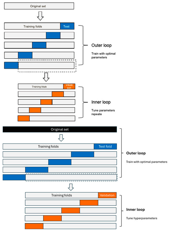
Figure 2.
Illustration of nested cross-validation. The black segment represents the original dataset. The gray segments indicate the training folds used in the outer and inner loops. The blue segments denote the test folds in the outer loop, while the orange segments represent the validation folds in the inner loop. The dashed lines indicate the selected training folds from the outer loop that are used to conduct the inner loop. The arrows illustrate the nested structure between the original dataset, the outer loop and the inner loop.
The outer cross-validation, which also used repeated stratified 5-fold splits (5 folds repeated 5 times), involved executing a grid search on each training split and then evaluating the best model on the held-out outer test fold. This process provided an unbiased estimate of the model’s generalization performance and generated confusion matrices that were averaged and reported with their standard deviations. Finally, the model selected from the nested cross-validation was evaluated on a separate held-out test set, with the training and test accuracies compared to confirm that the model generalized well to unseen data. For each algorithm, the performance metrics, including the accuracy, macro precision, macro recall, macro F1-score, and ROC-AUC [50], were reported as the mean ± standard deviation for both the inner and outer loops. In total, the overall nested cross-validation procedure involved 5 × 5 (inner) × 5 × 5 (outer) = 625 fits, along with the grid search, providing a stable and accurate estimation of the model performance.
Finally, given that the machine learning algorithms employed in the present study varied in terms of their result interpretability (e.g., linear models are more interpretable than ensemble methods), the XAI method [51] was used to gain a better understanding of feature importance. The open-source Python package (version 3.13.1), SHAP (Shapley additive explanations; version 0.45.0), was used for the XAI analysis. The core concept of the SHAP package is the SHAP (i.e., Shapley) values, which are derived from cooperative game theory and indicate the contribution or importance of each feature to the prediction of the model, rather than the quality of the prediction itself [52]. The current study used two main plots from the SHAP package: the SHAP summary plot and the SHAP-dependent plot. The SHAP summary plot displays the absolute value of feature importance for predicting the outcome variable and each of its classes, but it does not indicate the direction of the effect. The SHAP dependence plots were employed to obtain a deeper understanding of the direction of the effect. In a dependence plot, each participant is represented as a single point. The points are presented as a scatterplot of a variable’s SHAP values versus the variable’s underlying raw values. The shapes of the distributions of points provide insights into the relationship between a variable’s values and its SHAP values. Positive SHAP values lead to predictions of the corresponding enrollment status. All the machine learning model building and testing procedures were conducted in Python.
4. Results
This section presents the results of the analysis, including the performance metrics of the five algorithms evaluated. These metrics encompass the confusion matrix, accuracy, precision, recall, F1-score, and ROC-AUC score. Additionally, this section highlights the feature importance of the top ten predictors and examines the patterns through which the top five features influence each level of college enrollment.
4.1. Model Performance
The fine-tuned hyperparameters for each algorithm were as follows: for LR, the optimal values were a cost parameter (C) of 0.01 and an L2 penalty; for KNN, the optimal settings were 1 neighbor (n_neighbors = 1) with a Manhattan distance (p = 1); for the SVM, the optimal parameters were a cost (C) of 10, a gamma of 0.1, and an RBF kernel; for the DT, the optimal maximum depth was 7; and for RF, the optimal number of estimators was 10,000. Table 1 presents the model performance metrics obtained during the inner-loop cross-validation for each algorithm. Based on these fine-tuned hyperparameters, the outer loop was then used to select the most optimal classifier, with its performance metrics also summarized in Table 1. The confusion matrices for the five classifiers from the outer loop are shown in Figure 3, while the category-specific classification performance is illustrated by the ROC-AUC plots in Figure 4. Overall, the results indicate that random forests outperformed the other classifiers across all five evaluation metrics, the confusion matrix, and the ROC-AUC class-specific prediction. Finally, the optimal random forest classifier was applied to the held-out test dataset, yielding an accuracy of 67.73%, which was slightly lower than, but comparable to, the training set accuracy of 69.93%. These findings suggest that the random forest model does not suffer from overfitting.

Table 1.
Results of the classification performance evaluation in the inner and outer loops.
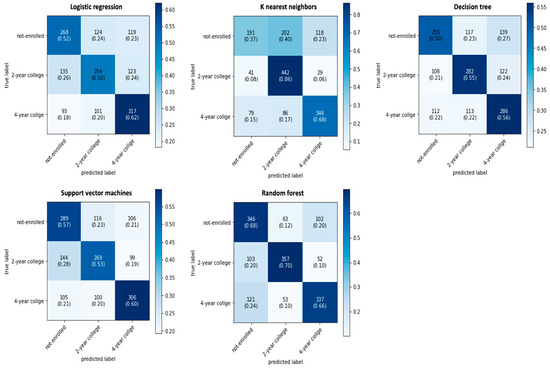
Figure 3.
The confusion matrices of the five classifiers.
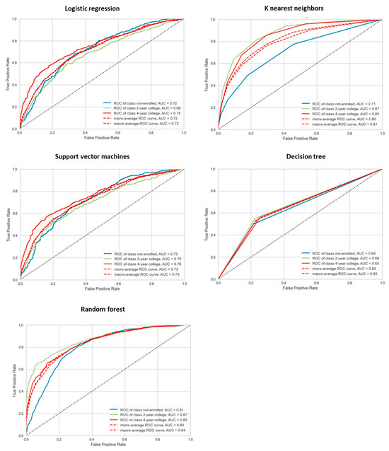
Figure 4.
The class-specific ROC-AUC curves of five classifiers.
4.2. Feature Importance
As shown in Figure 5, the top 10 important features for predicting college enrollment status were the high school GPA, parental educational expectations, the number of close friends who plan to attend a 4-year college, the students’ school motivation, the students’ school engagement, the number of close friends who dropped out of high school, the students’ educational expectations, the number of close friends who plan to attend a 2-year college, the students’ sense of school belonging, and the administrators’ assessment of school problems. Moreover, this plot displays the relative importance of the ten variables for predicting each college enrollment status (i.e., not enrolled, enrolled in a 2-year or less college, and enrolled in a 4-year college). The three most important factors for predicting student enrollment in 2-year and 4-year colleges were the high school GPA, parental educational expectations, and the number of close friends who plan to attend a 4-year college. In addition, the high school GPA, parental educational expectations, and the number of close friends who dropped out of high school were the top three predictors of students not enrolling in college.
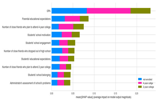
Figure 5.
SHAP summary plot for the multi-class classification.
The SHAP-dependent plot shows the relationship between each variable and its SHAP value for each enrollment status (see Figure 6). There was a negative, quadratic, and positive correlation between the high school GPA and the SHAP values for each enrollment status, with the highest SHAP values occurring for a GPA = 0.5 for those who were not enrolled in any institutions, GPA = 2.8 for those who were enrolled at a 2-year institution, and GPA = 3.5 for those who were enrolled at a 4-year institution. Similarly, there was still a negative, quadratic, and positive correlation between parental educational expectations and the SHAP values for each enrollment status. The highest SHAP values corresponded with expectations = 2 (i.e., expectation of obtaining a high school diploma or GED) for those who were not enrolled in any institutions, with expectations = 5 (i.e., expectation of starting a bachelor’s degree) for those who were enrolled in a 2-year institution, and with expectations = 10 (i.e., expectation of earning a Ph.D./M.D./law degree/other professional degree) for those who were enrolled in a 4-year institution. The number of close friends who plan to attend a 4-year college (0 = none of them, 1 = less than half, 2 = about half, 3 = more than half, 4 = all of them) had a negative relationship with the SHAP value for not enrolling in college and enrollment in a 2-year college, but a positive relationship with enrollment in a 4-year college. Finally, the relationship between student school motivation, school engagement, and their SHAP values were similar, with a negative association for those not enrolled in college, positive association values for those enrolled in a 4-year college, and an unclear pattern for those enrolled in a 2-year college. These findings indicate that enhanced school motivation and engagement are associated with both a reduced likelihood of college non-enrollment and an increased probability of enrollment in a 4-year college.
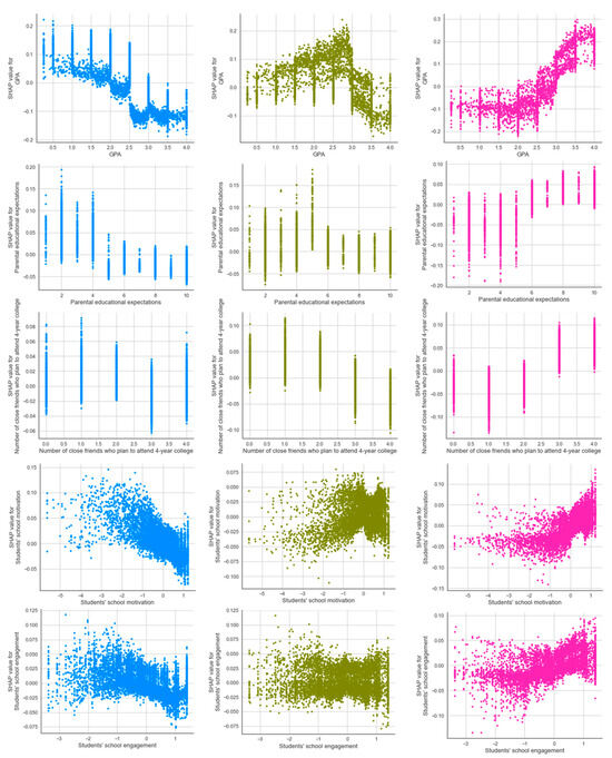
Figure 6.
SHAP dependence plot. All the above figures are scatter plots, where the colored dots represent individual data points.
5. Discussion
The current study identified the top ten actionable predictors of high school students’ college enrollment using the best-performing machine learning algorithm, random forest, out of all the classifiers compared and contrasted in this study. Of these ten predictors, five were student characteristics (i.e., high school GPA, school motivation, school engagement, educational expectation, and a sense of school belonging); three were peer characteristics (i.e., number of close friends who plan to attend a 4-year college, number of close friends who plan to attend a 2-year college, and number of close friends who dropped out of high school), which could be viewed as two main categories (i.e., close friends’ college plan and high school enrollment status); one was parental characteristics (i.e., parental educational expectations); and one was school characteristics (i.e., administrator’s assessment of school problems).
These results align with both the existing literature and the ecological system theory emphasizing that individual characteristics (e.g., ability, motivation, attitudes) exert a greater influence on college enrollment than microsystem factors like family, peers, or school environments in the ecological system theory [37]. These findings suggest that practitioners should prioritize developing students’ own competencies, expectations, motivation, and engagement through targeted interventions. Moreover, in terms of the relative importance of parents and peers on students’ college enrollment, although three variables were related to peers, parental educational expectations were more influential than all three peer characteristics. This result supports the claim that peers (friends) tend to have a somewhat greater influence on the broader range of developmental choices and short-term (or lifestyle) developmental choices, whereas parents tend to have a stronger overall influence on choices with longer-term developmental consequences [53].
In addition, this study indicated that students’ overall high school GPA is the most influential factor affecting their college enrollment. The relationship between GPA and its importance for the three enrollment statuses varied, with a negative pattern for no enrollment, a quadratic pattern for 2-year or less college enrollment, and a positive pattern for 4-year college enrollment. Although these patterns appear confusing at first glance, they make sense because students with a lower GPA may not be admitted to college, whereas those with a higher GPA are more likely to attend a 4-year college than a 2-year or less institution. More specifically, students with a GPA of 3.5 or above were more likely to be enrolled in a 4-year college, while those with a GPA between 2.5 and 3 were more likely to be enrolled in a 2-year or less college program, and those with a GPA of less than 0.5 were more likely to not be enrolled in any college program. This result is also consistent with that of Slim et al. [32]. Using support vector machines, they observed that applicants with a high school GPA between 3.0 and 3.50 were more likely to enroll at the University of New Mexico, a 4-year institution, than other applicants. It would be interesting if future research utilized machine learning algorithms to investigate more fine-grained research issues, such as comparing the difference in GPA scores across schools, regions, and countries.
Furthermore, among the top ten predictors, four of them were future-oriented goals (i.e., parental educational expectations, students’ educational expectations, close friends’ plans to attend 2-year college, and close friends’ plans to attend 4-year college). According to the model of future-oriented motivation and self-regulation proposed by Miller and Brickman [54], future-oriented goals are self-relevant, self-defining long-term goals that provide incentive for action. These goals include, but are not limited to, important personal aspirations such as obtaining an education, striving for a career or job, developing intimate personal relationships, and making a contribution to society. The good news for educational practitioners is that the emergence of future goals is typically viewed as part of the developmental process that occurs in an individual’s sociocultural context, including the home, peers, school, and media, which are known to shape individual values. In other words, this implies that we could encourage students to commit themselves to meaningful long-term educational goals and seek to benefit from their educational experiences, which would lead them to monitor their progress toward their goals, make necessary adjustments to their efforts, and establish new, more demanding goals as they accomplish earlier ones.
To the best of our knowledge, the current study is the first to use machine learning to identify the contributory factors of low-SES students’ college enrollment. Under the guidance of ecological system theory, we identified the ten most important actionable predictors out of a hundred and revealed their distinct patterns of prediction for three college enrollment statuses. These findings suggest some practical implications for educational practitioners. Specifically, educational practitioners could focus more on students’ high school GPAs to increase their overall college enrollment rate. In addition, parents could actively foster college expectations through regular participation in school activities, explicit discussions about post-secondary plans, and the consistent reinforcement of high academic standards. Moreover, educators and administrators can strengthen student motivation and engagement by implementing evidence-based strategies such as growth mindset training, college-focused mentoring programs, and classroom interventions that connect coursework to career pathways. A coordinated approach addressing both individual development and environmental supports will be most effective in promoting college enrollment.
6. Limitations and Future Work
This study has several limitations. First, because the original HSLS dataset contained more than a thousand variables, the features of interest were manually selected based on ecological system theory, the results of past studies, and the researchers’ prior expertise. This means that other important predictors of college enrollment might have been overlooked. This limited variable selection could be a potential reason for the modest model performance across all five algorithms. Future studies could explore more predictors based on the literature and theories. Second, this study utilized data from a nationally representative longitudinal study in the United States. Considering that the results of machine learning algorithms are subject to the input dataset, future studies could include data from other projects or nations to validate the results. In addition, due to the underrepresentation of low-SES students in college, the present study only focused on identifying predictors for increasing low-SES individuals’ college enrollment, posting a challenge for generalizing the results to the whole population. Future research might examine the predictors for high-SES students and compare and contrast the predictors for low- and high-SES students. Third, in terms of the interpretability of the model, the feature importance was obtained using the SHAP package. However, the SHAP value was used to evaluate the contribution or importance of each feature to the prediction of the model, rather than the quality of the prediction itself. Future studies may explore alternative ways to improve the model’s interpretability. Finally, while this study identified the key predictors of college enrollment among low-SES students, it did not examine intervention strategies based on these factors. Future research could employ experimental or quasi-experimental designs to both validate these findings and test the efficacy of interventions targeting these predictive factors.
7. Conclusions
This study identified the key predictors for low-SES high school students’ college enrollment based on the machine learning approach. The random forest algorithm outperformed the other four classifiers in predicting low-SES students’ college enrollment status, with an accuracy of 70% and an F1-score of 0.7. Furthermore, the student’s high school GPA as well as the students’, parents’, and friends’ future-oriented goals were revealed to be powerful factors in their college enrollment status. To the best of our knowledge, the current study is the first to systematically examine the contributing factors of low-SES students’ college enrollment using machine learning. The findings from the current study imply two practical implications for educational practitioners: (1) they may focus more on students’ high school GPA to enhance the overall college enrollment rate and (2) they could attempt to raise the educational attainment expectations of students, their friends, and their families.
Author Contributions
Conceptualization, S.H.; methodology, S.H. and M.C.; software, S.H.; validation, M.Y.-N.; formal analysis, S.H.; investigation, S.H.; resources, S.H.; data curation, S.H.; writing—original draft preparation, S.H. and M.C.; writing—review and editing, S.H., M.Y.-N., Y.C. and M.C.; visualization, S.H.; supervision, Y.C. and M.C.; project administration, S.H. All authors have read and agreed to the published version of the manuscript.
Funding
This research received no external funding.
Data Availability Statement
The dataset used in this study is publicly available on the official website of the National Center for Education Statistics: https://nces.ed.gov/surveys/hsls09/ (accessed on 10 April 2025).
Conflicts of Interest
The authors declare no conflicts of interest.
References
- Bates, L.A.; Anderson, P.D. Do expectations make the difference? A look at the effect of educational expectations and academic performance on enrollment in post-secondary education. Race Soc. Probl. 2014, 6, 249–261. [Google Scholar] [CrossRef]
- Eccles, J.S.; Vida, M.N.; Barber, B. The relation of early adolescents’ college plans and both academic ability and task-value beliefs to subsequent college enrollment. J. Early Adolesc. 2004, 24, 63–77. [Google Scholar] [CrossRef]
- Fraysier, K.; Reschly, A.; Appleton, J. Predicting postsecondary enrollment with secondary student engagement data. J. Psychoeduc. Assess. 2020, 38, 882–899. [Google Scholar] [CrossRef]
- Cheatham, G.A.; Elliott, W. The effects of family college savings on postsecondary school enrollment rates of students with disabilities. Econ. Educ. Rev. 2013, 33, 95–111. [Google Scholar] [CrossRef]
- Degol, J.L.; Wang, M.T.; Ye, F.; Zhang, C. Who makes the cut? Parental involvement and math trajectories predicting college enrollment. J. Appl. Dev. Psychol. 2017, 50, 60–70. [Google Scholar] [CrossRef]
- Johnson, P.M.; Newman, L.A.; Cawthon, S.W.; Javitz, H. Parent expectations, deaf youth expectations, and transition goals as predictors of postsecondary education enrollment. Career Dev. Transit. Except. Individ. 2022, 45, 131–142. [Google Scholar] [CrossRef]
- Lessard, L.M.; Juvonen, J. Developmental changes in the frequency and functions of school-related communication with friends and family across high school: Effects on college enrollment. Dev. Psychol. 2022, 58, 575–583. [Google Scholar] [CrossRef]
- Sokatch, A. Peer influences on the college-going decisions of low socioeconomic status urban youth. Educ. Urban Soc. 2006, 39, 128–146. [Google Scholar] [CrossRef]
- Belasco, A.S. Creating college opportunity: School counselors and their influence on postsecondary enrollment. Res. High. Educ. 2013, 54, 781–804. [Google Scholar] [CrossRef]
- Engberg, M.E.; Wolniak, G.C. Examining the effects of high school contexts on postsecondary enrollment. Res. High. Educ. 2010, 51, 132–153. [Google Scholar] [CrossRef]
- Peter, F.H.; Zambre, V. Intended college enrollment and educational inequality: Do students lack information? Econ. Educ. Rev. 2017, 60, 125–141. [Google Scholar] [CrossRef]
- Ou, S.R.; Reynolds, A.J. Predictors of educational attainment in the Chicago Longitudinal Study. Sch. Psychol. Q. 2008, 23, 199. [Google Scholar] [CrossRef]
- Bureau of Labor Statistics, U.S. Department of Labor. The Economics Daily: High School Graduates with No College had Unemployment Rate of 4.5 Percent in February 2022. Available online: https://www.bls.gov/opub/ted/2022/high-school-graduates-with-no-college-had-unemployment-rate-of-4-5-percent-in-february-2022.htm (accessed on 6 March 2025).
- Wolla, S.A.; Sullivan, J. Education, Income, and Wealth. Page One Economics. Available online: https://www.stlouisfed.org/publications/page-one-economics/2017/01/03/education-income-and-wealth (accessed on 6 March 2025).
- Shrider, E.A.; Kollar, M.; Chen, F.; Semega, J. Income and Poverty in the United States: 2020; US Census Bureau: Suitland, MD, USA, 2021.
- Guzman, G.; Kollar, M. Income in the United States: 2023 (Current Population Reports, P60–282); U.S. Census Bureau; U.S. Government Publishing Office: Suitland, MD, USA, 2024. Available online: https://www.census.gov/library/publications/2024/demo/p60-282.html (accessed on 6 March 2025).
- Juszkiewicz, J. Trends in Community College Enrollment and Completion Data; American Association of Community Colleges; The Institute of Education Sciences of the U.S. Department of Education: Washington, DC, USA, 2020.
- Tate, T.; Warschauer, M. Equity in online learning. Educ. Psychol. 2022, 57, 192–206. [Google Scholar] [CrossRef]
- Tsai, C.L.; Brown, A.; Lehrman, A.; Tian, L. Motivation and postsecondary enrollment among high school students whose parents did not go to college. J. Career Dev. 2022, 49, 411–426. [Google Scholar] [CrossRef]
- Slaten, C.D.; Ferguson, J.K.; Allen, K.A.; Brodrick, D.V.; Waters, L. School belonging: A review of the history, current trends, and future directions. Educ. Dev. Psychol. 2016, 33, 1–15. [Google Scholar] [CrossRef]
- Perez, P.A.; McDonough, P.M. Understanding Latina and Latino college choice: A social capital and chain migration analysis. J. Hisp. High. Educ. 2008, 7, 249–265. [Google Scholar] [CrossRef]
- Person, A.E.; Rosenbaum, J.E.; Deil-Amen, R. Student planning and information problems in different college structures. Teach. Coll. Rec. 2006, 108, 374–396. [Google Scholar] [CrossRef]
- Perna, L.W.; Titus, M.A. The relationship between parental involvement as social capital and college enrollment: An examination of racial/ethnic group differences. J. High. Educ. 2005, 76, 485–518. [Google Scholar] [CrossRef]
- Rowan-Kenyon, H.T.; Bell, A.D.; Perna, L.W. Contextual influences on parental involvement in college going: Variations by socioeconomic class. J. High. Educ. 2008, 79, 564–586. [Google Scholar] [CrossRef]
- Stimpson, M.T.; Janosik, S.M.; Miyazaki, Y. Examining social capital as a predictor of enrollment in four-year institutions of postsecondary education for low socioeconomic status students. Enroll. Manag. J. 2010, 4, 34–56. [Google Scholar]
- Stephan, J.L.; Rosenbaum, J.E. Can high schools reduce college enrollment gaps with a new counseling model? Educ. Eval. Policy Anal. 2013, 35, 200–219. [Google Scholar] [CrossRef]
- Sciarra, D.T.; Ambrosino, K.E. Post-secondary expectations and educational attainment. Prof. Sch. Couns. 2011, 14, 2156759X1101400. [Google Scholar] [CrossRef]
- Knight, D.S.; Duncheon, J.C. Broadening conceptions of a “college-going culture”: The role of high school climate factors in college enrollment and persistence. Policy Futures Educ. 2020, 18, 314–340. [Google Scholar] [CrossRef]
- Linsenmeier, D.M.; Rosen, H.S.; Rouse, C.E. Financial aid packages and college enrollment decisions: An econometric case study. Rev. Econ. Stat. 2006, 88, 126–145. [Google Scholar] [CrossRef]
- Nielsen, H.S.; Sørensen, T.; Taber, C. Estimating the effect of student aid on college enrollment: Evidence from a government grant policy reform. Am. Econ. J. Econ. Policy 2010, 2, 185–215. [Google Scholar] [CrossRef]
- Ragab, A.H.M.; Noaman, A.Y.; Al-Ghamdi, A.S.; Madbouly, A.I. A comparative analysis of classification algorithms for students college enrollment approval using data mining. In Proceedings of the IDEE ’14: Interaction Design in Educational Environments, Albacete, Spain, 9 June 2014; Association for Computing Machinery: New York, NY, USA, 2014. [Google Scholar]
- Slim, A.; Hush, D.; Ojah, T.; Babbitt, T. Predicting student enrollment based on student and college characteristics. In Proceedings of the 11th International Conference on Educational Data Mining, EDM, Buffalo, NY, USA, 15–18 July 2018; International Educational Data Mining Society: Worcester, MA, USA, 2018. [Google Scholar]
- Yang, L.; Feng, L.; Zhang, L.; Tian, L. Predicting freshmen enrollment based on machine learning. J. Supercomput. 2021, 77, 11853–11865. [Google Scholar] [CrossRef]
- Ujkani, B.; Minkovska, D.; Stoyanova, L. A machine learning approach for predicting student enrollment in the university. In Proceedings of the 2021 International Scientific Conference Electronics (ET), Sozopol, Bulgaria, 15–17 September 2021. [Google Scholar]
- Bronfenbrenner, U. Ecological Systems Theory; Jessica Kingsley Publishers: London, UK, 1992. [Google Scholar]
- Bronfenbrenner, U. The Ecology of Human Development; Harvard University Press: Cambridge, MA, USA, 2009. [Google Scholar]
- Espelage, D.L. Ecological theory: Preventing youth bullying, aggression, and victimization. Theory Into Pract. 2014, 53, 257–264. [Google Scholar] [CrossRef]
- Gunning, D.; Aha, D. DARPA’s explainable artificial intelligence (XAI) program. AI Mag. 2019, 40, 44–58. [Google Scholar] [CrossRef]
- Pasquale, F. The Black Box Society: The Secret Algorithms that Control Money and information; Harvard University Press: Cambridge, MA, USA, 2015. [Google Scholar] [CrossRef]
- Bulut, O.; Wongvorachan, T.; He, S.; Lee, S. Enhancing High-School Dropout Identification: A Collaborative Approach Integrating Human and Machine Insights. Discov. Educ. 2024, 3, 109. [Google Scholar] [CrossRef]
- Rudin, C. Stop explaining black box machine learning models for high stakes decisions and use interpretable models instead. Nat. Mach. Intell. 2019, 1, 206–215. [Google Scholar] [CrossRef]
- Zhang, L.; Lin, Y.; Yang, X.; Chen, T.; Cheng, X.; Cheng, W. From sample poverty to rich feature learning: A new metric learning method for few-shot classification. IEEE Access 2024, 12, 124990–125002. [Google Scholar] [CrossRef]
- Minh, D.; Wang, H.X.; Li, Y.F.; Nguyen, T.N. Explainable artificial intelligence: A comprehensive review. Artif. Intell. Rev. 2022, 55, 3503–3568. [Google Scholar] [CrossRef]
- Bowers, A.J. Early warning systems and indicators of dropping out of upper secondary school: The emerging role of digital technologies. In OECD Digital Education Outlook 2021: Pushing the Frontiers with Artificial Intelligence, Blockchain and Robots; OECD Publishing: Paris, France, 2021; pp. 173–194. [Google Scholar] [CrossRef]
- Tang, A.K.; Ng, K.M. High school counselor contacts as predictors of college enrollment. Prof. Couns. 2019, 9, 347–357. [Google Scholar] [CrossRef]
- Fonti, V.; Belitser, E. Feature Selection Using Lasso; VU Amsterdam Research Paper in Business Analytics; Vrije Universiteit Amsterdam: Amsterdam, The Netherlands, 2017; Volume 30, pp. 1–25. Available online: https://www.researchgate.net/profile/David-Booth-7/post/Regression-of-pairwise-trait-similarity-on-similarity-in-personal-attributes/attachment/5b18368d4cde260d15e3a4e3/AS%3A634606906785793%401528313485788/download/werkstuk-fonti_tcm235-836234.pdf (accessed on 10 April 2025).
- Chawla, N.V.; Bowyer, K.W.; Hall, L.O.; Kegelmeyer, W.P. SMOTE: Synthetic minority over-sampling technique. J. Artif. Intell. Res. 2002, 16, 321–357. [Google Scholar] [CrossRef]
- Jung, Y. Multiple predicting K-fold cross-validation for model selection. J. Nonparamet. Stat. 2018, 30, 197–215. [Google Scholar] [CrossRef]
- Tsamardinos, I.; Rakhshani, A.; Lagani, V. Performance-estimation properties of cross-validation-based protocols with simultaneous hyper-parameter optimization. Int. J. Artif. Intell. Tools 2015, 24, 1540023. [Google Scholar] [CrossRef]
- Novaković, J.D.; Veljović, A.; Ilić, S.S.; Papić, Ž.; Milica, T. Evaluation of classification models in machine learning. Theory Appl. Math. Comput. Sci. 2017, 7, 39–46. Available online: https://uav.ro/applications/se/journal/index.php/TAMCS/article/view/158 (accessed on 10 April 2025).
- Linardatos, P.; Papastefanopoulos, V.; Kotsiantis, S. Explainable ai: A review of machine learning interpretability methods. Entropy 2020, 23, 18. [Google Scholar] [CrossRef]
- Lundberg, S.M.; Lee, S.I. A unified approach to interpreting model predictions. In Proceedings of the 31st Conference on Neural Information Processing Systems (NIPS 2017), Long Beach, CA, USA, 4–9 December 2017; Available online: https://papers.nips.cc/paper/7062-a-unified-approach-to-interpreting-model-predictions (accessed on 10 April 2025).
- Wang, A.; Peterson, G.W.; Morphey, L.K. Who is more important for early adolescents’ developmental choices? Peers or parents? Marriage Fam. Rev. 2007, 42, 95–122. [Google Scholar] [CrossRef]
- Miller, R.B.; Brickman, S.J. A model of future-oriented motivation and self-regulation. Educ. Psychol. Rev. 2004, 16, 9–33. [Google Scholar] [CrossRef]
Disclaimer/Publisher’s Note: The statements, opinions and data contained in all publications are solely those of the individual author(s) and contributor(s) and not of MDPI and/or the editor(s). MDPI and/or the editor(s) disclaim responsibility for any injury to people or property resulting from any ideas, methods, instructions or products referred to in the content. |
© 2025 by the authors. Licensee MDPI, Basel, Switzerland. This article is an open access article distributed under the terms and conditions of the Creative Commons Attribution (CC BY) license (https://creativecommons.org/licenses/by/4.0/).