From Rating Predictions to Reliable Recommendations in Collaborative Filtering: The Concept of Recommendation Reliability Classes

Abstract

Recommender systems aspire to provide users with recommendations that have a high probability of being accepted. This is accomplished by producing rating predictions for products that the users have not evaluated, and, afterwards, the products with the highest prediction scores are recommended to them. Collaborative filtering is a popular recommender system technique which generates rating prediction scores by blending the ratings that users with similar preferences have previously given to these products. However, predictions may entail errors, which will either lead to recommending products that the users would not accept or failing to recommend products that the users would actually accept. The first case is considered much more critical, since the recommender system will lose a significant amount of reliability and consequently interest. In this paper, after performing a study on rating prediction confidence factors in collaborative filtering, (a) we introduce the concept of prediction reliability classes, (b) we rank these classes in relation to the utility of the rating predictions belonging to each class, and (c) we present a collaborative filtering recommendation algorithm which exploits these reliability classes for prediction formulation. The efficacy of the presented algorithm is evaluated through an extensive multi-parameter evaluation process, which demonstrates that it significantly enhances recommendation quality.

1. Introduction

Collaborative filtering (CF) has become one of the most widely used methods in recommender systems (RecSys) in recent years. CF predicts rating values for items that users have not already rated by blending the rating values that users with similar rating behaviors have given to the same items. In CF, these users are termed near neighbors (NNs) [1,2].

More specifically, in the initial step of a CF RecSys, the similarities between users are computed, using a vicinity metric. In CF research, the most commonly used metrics are the Cosine Similarity and the Pearson Correlation [3,4]. Then, for each user, the users found to have the highest vicinity metric values, and, therefore, who will play the role of the current user’s NNs, are selected. The most popular techniques for selecting NNs are the top-K method and the vicinity metric threshold method [5,6]. In the first technique, the set of NNs contains the K users with the largest vicinity value (K is a parameter of the method). In the second technique, the set of NNs contains all users whose vicinity surpasses a preset threshold value THR (which is a parameter of the technique). Consequently, for each item that the user has not rated yet, the ratings of their NNs for the same item are combined to generate the numeric prediction value. Combination can be performed using a weighted average formula, where the weight for each NN’s rating is equal to the similarity between the current user and the specific NN. In the last step of a CF RecSys, typically, the items that achieve the highest prediction arithmetic values, for each user, are finally recommended to them [7,8]. The number of items included in the recommendation is a parameter of the RecSys.

For example, let us assume that for a user U, there are only two candidate items for recommendation, i₁ and i₂. The rating prediction value of item i₁, pr₁, is computed at 4.9/5, while the rating prediction value of item i₂, pr₂, is computed at 4.7/5, and hence a typical CF RecSys will recommend i₁ over i₂ to U, based only on the rating prediction value. However, if we know or we can compute the confidence of each prediction formulation, the final recommendation could be different. For example, if pr₁ is found to have low confidence (for example, it is based on only one U’s NN), whereas pr₂ is found to have high confidence (for example, it is based on 15 Us NNs), recommending item i₂ appears a more appropriate choice, since its prediction value is also very high (4.7/5) and additionally it seems almost certain and safe.

Towards this direction, recent studies have demonstrated that an association exists between rating prediction accuracy and the specific characteristics of individual rating predictions in CF [9,10]. These works indicate that the following characteristics (also termed “factors”) are strongly correlated with high accuracy in CF rating prediction: (a) the number of NNs contributing to the prediction formulation, (b) the user’s average ratings value, and (c) the item’s average ratings value.

In this work, after performing a study on rating prediction confidence factors in CF, (a) we introduce the concept of prediction reliability classes; (b) we formulate a total ordering of these classes, which is associated with the utility of the rating predictions belonging to each class; and (c) we present a CF recommendation algorithm that prioritizes the rating predictions which are classified in higher recommendation reliability class(es) when making its recommendations. This algorithm bestows the RecSys administrator with the ability to adjust the level of recommendation quality and/or coverage s/he needs. The adjustment only utilizes essential CF data, and thus, it can be applied in every CF RecSys dataset. We substantiate the efficacy of the presented algorithm through an extensive multi-parameter evaluation process, using (a) both the Cosine Similarity and the Pearson Correlation vicinity metrics, (b) both the top-K and the correlation threshold methods for NN selection, and (c) eight CF datasets from multiple sources.

The remainder of the paper is organized as follows: in Section 2 we summarize the related work, and in Section 3 we briefly set out the foundations of this work. In Section 4 we perform a study on rating prediction confidence factors in CF, and in Section 5 we introduce the concept of recommendation reliability classes and consequently the proposed algorithm. In Section 6 we present the evaluation results, and in Section 7 we discuss these results. Finally, in Section 8 we conclude the paper and summarize our future work.

2. Related Work

CF recommendation quality is a research subject targeted by plenty of studies in the last 10 years. The works on this subject are divided into two major categories; the first consists of studies that consider only the basic CF input information (i.e., the users’ ratings of items, including the time the rating took place). The second category consists of works that consider enriched input information (i.e., the basic information, along with user demographics and/or social relations, item categories and/or features, etc.).

Regarding the first category, Liao and Lee [11] propose a CF technique that minimizes the dimensionality of products by employing a clustering algorithm. Specifically, this approach assigns dissimilar items to separate clusters, while grouping similar items together. Following this, a list of recommended items in rank order is provided to each person. Diaz et al. [12] introduce a Bayesian CF method that provides explanations for the generated recommendations. This algorithm incorporates both item-based and user-based CF methods, merging them into a unified user–item approach. Margaris and Vassilakis [13] introduce a CF-based technique which eliminates outdated user evaluations from the database, assuming that they no longer accurately reflect the users’ current preferences. This algorithm can be implemented in an unsupervised manner and has been shown to improve rating prediction accuracy while also reducing the size of the CF rating database. Neysiani et al. [14] propose a weighted quality CF metric which aims to overcome the problem of multi-objective rule mining. This metric uses genetic algorithms to exploit confidence in and support of association rules. The application of the genetic algorithm enables rapid discovery of association rules. Thakkar et al. [15] propose a CF algorithm which combines item and user predictions to generate CF predictions with minimal error. Furthermore, this algorithm incorporates both linear and support vector regressions. He et al. [16] present a modern recommendation algorithm based on Graph Convolution Networks, called LightGCN, which has been proved to outperform Neural Graph Collaborating Filtering (NGCF). LightGCN consists of two main components: a layer combination and a light graph convolution. The first simplifies the standard GCN approach by removing feature transformation and nonlinear activation operations, which typically add complexity to the training process. The second generates the concluding node embeddings by calculating the sum of the layers’ embeddings. Li et al. [17] introduce Decoupled Graph Neural Networks (DGNN), a method that integrates each product’s factor-level ratings with the session’s objective. This approach first uses disentangled learning to decompose item embeddings into factor embeddings. Then, it operates a graph neural network to effectively determine the factors. Wei et al. [18] present a Log-range Graph Transformer model, namely LGT, that determines user preference representation by establishing correlations between the products’ features. The model supports proximity calculation by incorporating modal-specific embedding and a layer-wise position encoder. Additionally, it uses a self-attention block to enhance the efficiency of self-attention scoring.

Considering the second major category, Yang et al. [19] suggest an approach which combines sparse rating data with trust network data among users, to enhance the performance of CF recommendations. Specifically, this method utilizes matrix factorization techniques to capture the impact of user opinion formation more precisely. Wang et al. [20] introduce a user similarity approach using a hybrid method that takes into account the influence of all evaluated products, the nonlinear relationships between variables, the users’ evaluating preferences, as well as their asymmetry. The framework for this approach is built upon a nonlinear formula, which overcomes the limitation of co-rated items and fully leverages all available ratings. The presented user similarity model, grounded in this framework, also incorporates additional factors, like user preferences and asymmetry. Islam et al. [21] explore gender bias in CF RecSys tested on social media information. To address this, they created the Neural Fair Collaborating Filtering (NFCF), a practical model designed to reduce gender bias in the recommendation of career-related sensitive items (e.g., courses of study, jobs, etc.). This model combines a fine-tuning and pre-training approach to neural CF with methods of bias correction.

Iwendi et al. [22] introduce a machine learning model CF algorithm that uses a rating scale of 0, 2, and 4 to evaluate items, where 0, 4, and 2 represent negative, positive, and neutral assessment. This new algorithm is designed to complement the existing review system that handles user comments and reviews, without disrupting it. The model was built utilizing Scikit-Learn, Pandas and Keras, and libraries to manage the internal processes. Chen et al. [23] introduce a CF RecSys algorithm for IoT systems, which is based on adaptive trust models. By using a sliding window and a time decay formula to calculate direct trust, the model significantly improves the trust evaluation convergence rate. A CF RecSys technique is designed to efficiently eliminate poor recommendations and reduce the strength of mischievous entities. Additionally, adaptive weight is introduced to effectively fuse recommendation trust with direct trust into a synthesized trust score, allowing the system to better adapt to a dynamically hostile environment.

Chang et al. [24] present a hybrid approach to generate personalized travel recommendations that better cater to individual travelers’ needs and enhance their online booking experience. This approach combines multi-attribute CF with social media data within a large-scale group decision-making framework. Specifically, k-means clustering and user filtering methods are employed to find user-experts for travel recommendation assignments. Consequently, community detection and social network construction are used to overcome the sparsity issue. Lastly, the travel options are sorted, and recommendations are selected in order to address the issue of cold start. Nguyen et al. [25] propose a hybrid recommendation approach that combines word embedding analysis with CF methods. The items’ content is represented through attributes like actors, directors, and plots, all centered around the movie subject. The primary goal of this study is to gain a deeper understanding of movie plot content using word embeddings, which improves the similarity measurement between different contents. To further enhance the accuracy of similarity measurement between movies, additional features like actors, directors, genres, and titles are also taken into account.

Rohit et al. [26] present a CF-based machine learning approach which produces recommendations to users. In this work, they use the Rapid Miner data, a machine learning mining tool for the tasks of research and analysis in data mining. This work achieves satisfactory results; however, it needs additional user and item information to function, such as user age, user location, item genre/category, etc. As a result, this approach cannot be applied in every dataset. Shambour [27] presents a multi-criteria deep learning RecSys algorithm that uses autoencoders to exploit the nonlinear, non-trivial, and hidden user relations. This work satisfactorily improves the recommendation accuracy; however, it needs additional user and item information to function, such as value for money, location, overall QoS, etc. As a result, this algorithm cannot be applied in every dataset.

However, the idea of using rating prediction certainty factors to improve recommendation quality in CF RecSys has still not been extensively explored. Recent studies have focused on rating prediction factors that are based solely on the very basic CF information, which are related to the accuracy of CF rating predictions. In particular, the works in [9,10] indicate that (a) the number of NNs contributing to the prediction formulation, (b) the user’s average ratings value, and (c) the item’s average ratings value are strongly correlated with high accuracy in CF rating prediction. Based on the aforementioned works, the work in Margaris et al. [28] prevents rating predictions with low confidence factor values and, hence, low certainty from becoming recommendations. Furthermore, the work in Sgardelis et al. [29] introduces a CF recommendation algorithm that allows for rating predictions with higher confidence factor values to outrank predictions with higher value, but lower confidence factor values.

While both these research works were found to upgrade CF recommendation quality, the first was found to significantly reduce recommendation coverage (i.e., the percentage of the users for whom recommendations can be generated), while the second was found to achieve marginal quality improvements (only a 2–3% enhancement).

In this work, we advance the state-of-the-art in CF RecSys research by (a) introducing the concept of recommendation reliability classes; (b) formulating a total ordering of these classes, which is associated with the utility of the rating predictions belonging to each class; and (c) presenting a CF recommendation algorithm which prioritizes the rating predictions which are classified in higher reliability class(es) when making its recommendations. This algorithm gives the RecSys administrator the ability to adjust the level of recommendation quality and/or coverage they need. Also, it is based only on the very basic CF information and is thus able to be applied in every CF RecSys dataset.

3. Foundations

In this section, the foundations of our work are briefly presented. In particular, the procedure of CF recommendation generation is presented in Section 3.1, and an overview of the factors that affect CF rating prediction accuracy is provided in Section 3.2.

3.1. CF Recommendation Generation Procedure

The procedure of CF recommendation generation formally includes the following four steps:

• The CF RecSys computes the vicinities (or distances) between all database/dataset users with the use of a vicinity metric. There is a plethora of vicinity metrics used in CF RecSys research, but the most commonly used are the Cosine Similarity and the Pearson Correlation [3,4];
• For each user, the CF RecSys selects the set of users (the NNs) who will act as the user recommenders. The NNs are typically the users who have the largest vicinity values with the user. The most commonly adopted techniques for selecting NNs are the top-K method (users with the K-highest vicinity metrics with target user U are selected as U’s NNs) and the correlation threshold method (users whose vicinity with target user U surpasses a threshold T are selected as U’s NNs) [5,6], as described in the Introduction Section;
• For each user, the CF RecSys tries to formulate predictions for every item the user has not rated yet. It does so by using a prediction formula that fuses the user NNs’ ratings of the same item into a single prediction value;
• Typically, for each user, the item(s) receiving the top rating prediction arithmetic score(s) is/are presented (suggested) to them.

3.2. CF Rating Prediction Accuracy Factors

Contemporary studies [9,10] have shown an association between CF rating prediction accuracy and the following three rating prediction confidence factors:

• The cardinality of NNs contributing to the prediction computation for the specific item (termed as F_NN). Note that, out of all the NNs of a user U, only the NNs that have rated an item i contribute to the computation of the prediction of the rating that U would assign to i. For sparse datasets, if F_NN ≥ 2, then the prediction is considered “accurate” and if F_NN ≥ 4, then the prediction is considered “very accurate”. The respective boundaries for dense datasets are 6% (“accurate”) and 15% (“very accurate”);
• The user’s average value of ratings (termed as F_{U_AVG}). For both dense and sparse datasets, when using a five-star evaluation scale, as happens in the majority of the CF RecSys datasets, if (F_{U_AVG} ≤ 2.0 OR F_{U_AVG} ≥ 4.0), then the prediction is considered “accurate”, and if (F_{U_AVG} ≤ 1.5 OR F_{U_AVG} ≥ 4.5), then the prediction is considered “very accurate”;
• The item’s average value of ratings (termed as F_{I_AVG}). The boundaries are exactly the same with the F_{U_AVG} factor, i.e., (F_{I_AVG} ≤ 2.0 OR F_{I_AVG} ≥ 4.0) for the “accurate” predictions and (F_{I_AVG} ≤ 1.5 OR F_{I_AVG} ≥ 4.5) for the “very accurate” predictions.

4. Experimental Settings and Evaluation Results of the Study on Rating Prediction Confidence Factors in CF

4.1. Experimental Settings and Procedure

In this study, we use eight datasets, including both sparse and dense, from four different sources and that are commonly utilized in CF research area to ensure generalizability. Table 1 lists these eight datasets, summarizing their attributes.

Furthermore, in this work we use both the Pearson Correlation (PC) and the Cosine Similarity (CS) user vicinity metrics (step 1 of the CF recommendation generation procedure, analyzed in Section 3.1). Additionally, we use both the top-K (TOP-K) and the correlation threshold methods (CT) for the NN selection (step 2 of the CF recommendation generation procedure, analyzed in Section 3.1). By considering multiple approaches in each step, we promote experimentation comprehensiveness and generalizability of results.

Regarding the TOP-K method, in our experiments we set K = 200 and K = 500. Regarding the CT method, we set T = 0.0 and T = 0.5, following the works in [1,6,28,29].

Regarding the rating prediction formulation, the five-fold cross validation approach is followed, a procedure commonly utilized in CF rating prediction research when using rating datasets [30,31,32,33].

Table 1. The datasets involved in our experiments, along with their basic attributes.

Name	Attributes
Amazon CDs_and_Vinyl [34]	112 K Users, 73.7 K items, 1.44 M ratings (range 1–5), 5-core, density 0.017% (sparse)
Amazon Musical Instruments [34]	27.5 K Users, 10.6 K items, 231 K ratings (range 1–5), 5-core, density 0.08% (sparse)
Amazon Videogames [34]	17.5 K users, 55 K items, 473 K ratings (range 1–5), 5-core, 0.05% density (sparse)
Amazon Digital Music [34]	12 K users, 17 K items, 145 K ratings (range 1–5), 5-core, 0.07% density (sparse)
CiaoDVD [35]	17.6 K users, 16 K items, 73 K ratings (range 1–5), 0.026% density (sparse)
Epinions [36]	22 K users, 296 K items, 922 K ratings (range 1–5), 0.014% density (sparse)
MovieLens 100K old [37]	1 K users, 1.7 K items, 100 K ratings (range 1–5), 5.88% density (dense)
MovieLens 1M [37]	6 K users, 3.7 items, 1 M ratings (range 1–5), 4.5% density (dense)

Table 1. The datasets involved in our experiments, along with their basic attributes.

Name	Attributes
Amazon CDs_and_Vinyl [34]	112 K Users, 73.7 K items, 1.44 M ratings (range 1–5), 5-core, density 0.017% (sparse)
Amazon Musical Instruments [34]	27.5 K Users, 10.6 K items, 231 K ratings (range 1–5), 5-core, density 0.08% (sparse)
Amazon Videogames [34]	17.5 K users, 55 K items, 473 K ratings (range 1–5), 5-core, 0.05% density (sparse)
Amazon Digital Music [34]	12 K users, 17 K items, 145 K ratings (range 1–5), 5-core, 0.07% density (sparse)
CiaoDVD [35]	17.6 K users, 16 K items, 73 K ratings (range 1–5), 0.026% density (sparse)
Epinions [36]	22 K users, 296 K items, 922 K ratings (range 1–5), 0.014% density (sparse)
MovieLens 100K old [37]	1 K users, 1.7 K items, 100 K ratings (range 1–5), 5.88% density (dense)
MovieLens 1M [37]	6 K users, 3.7 items, 1 M ratings (range 1–5), 4.5% density (dense)

In this work, we consider the following two RecSys evaluation metrics (following the works in [28,29,38,39]):

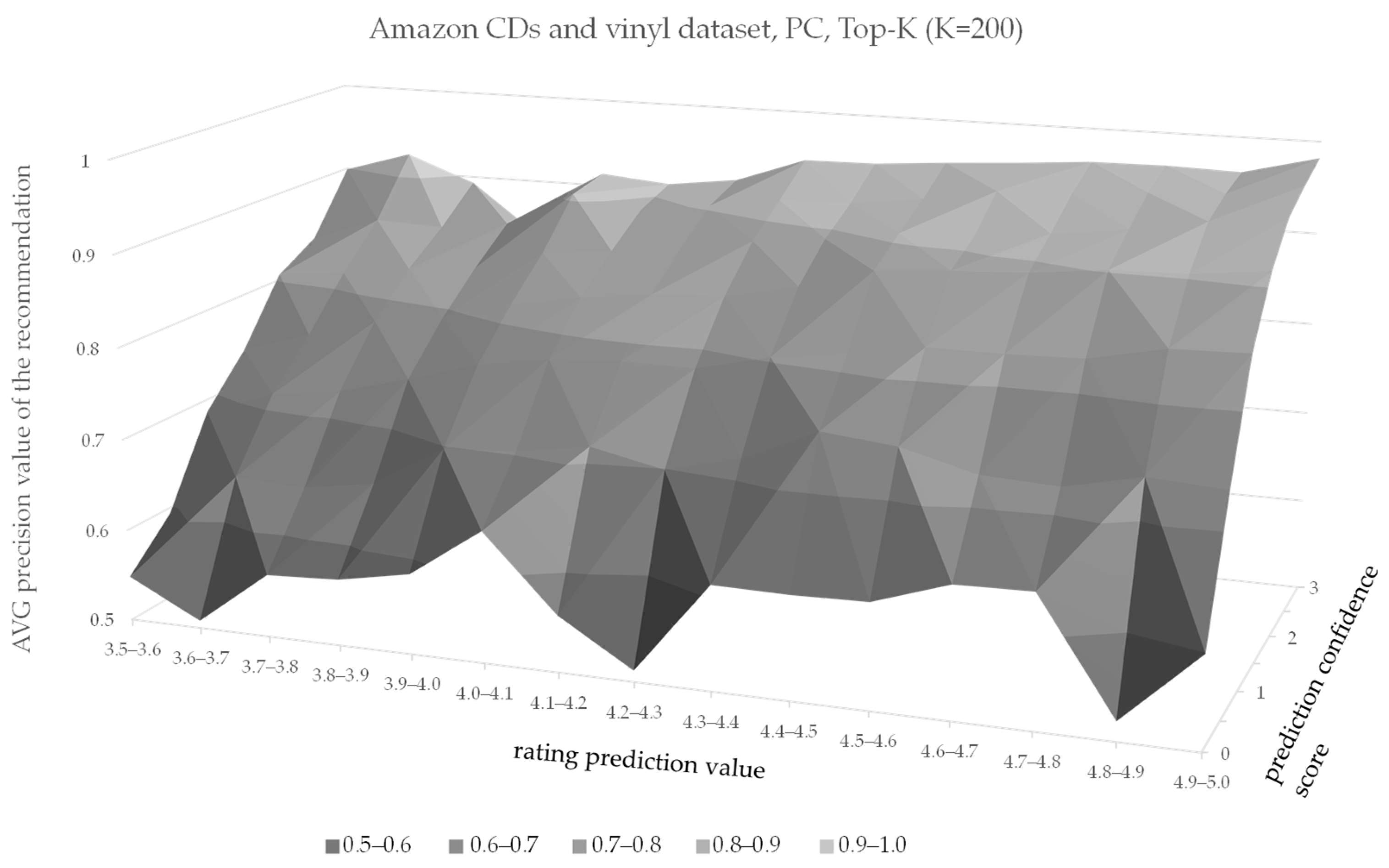
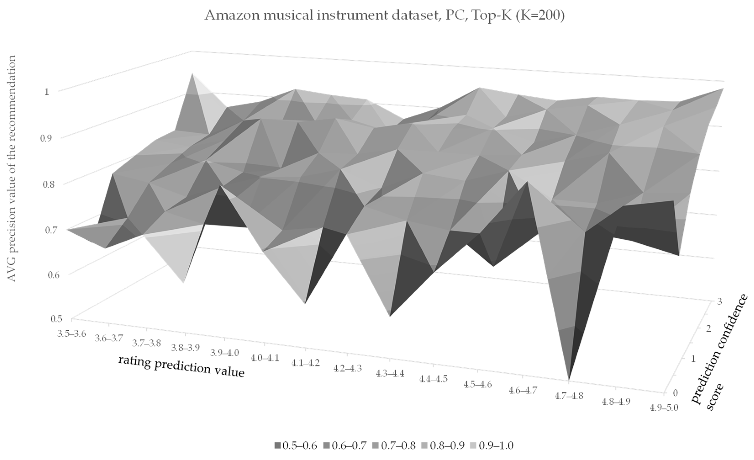
• The precision of the recommendations;
• The average actual arithmetic rating values of the items that have been recommended.

Regarding the number of recommended items, we use the top-1 and top-3, i.e., we first recommend one item to each user and subsequently three items. Furthermore, regarding the prediction and acceptance threshold of the recommended items, we follow the approach adopted in many research works [40,41,42], including the two works which will be used for comparison [28,29]. Based on this approach, the items with rating prediction scores in the upper 30% of the evaluation range (i.e., 3.5/5 for the five-star rating scale) can be recommended to the users. Similarly, the items whose actual rating is ≥3.5 are considered accepted/liked by the users.

4.2. Evaluation Results of the Study on Rating Prediction Confidence Factors in CF

The first step of this work is an experimental study of the association between (i) the arithmetic value of the rating prediction, (ii) the confidence factors satisfied by this prediction, and (iii) the actual-real rating value, in CF datasets. This experiment aims to provide insight that will enable the extraction of rules that can be used for prioritizing recommendations, effectively constituting the validation phase of the study, since the prioritization rules correspond to hyperparameters of the proposed algorithm. These rules will take into account (a) the rating prediction values, (b) the prediction accuracy factors associated with each prediction, and (c) the observed accuracy of these predictions.

In the first set of experiments, we use the first two datasets of Table 1, i.e., the Amazon CDs and Vinyl and the Amazon Musical Instruments. Furthermore, we exploit the three CF rating prediction accuracy factors analyzed in Section 3.2 to compute a partial confidence score for each of the rating prediction accuracy factors (number of NNs, user’s average value of ratings, and item’s average value of ratings) as follows:

• If the rating prediction fulfils the strict criterion for the specific factor (and is considered “very accurate”), we assign a factor-specific confidence score of 1.0 to the particular prediction;
• Otherwise, if the rating fulfills the loose criterion for the specific factor (and is thus considered “accurate”), we assign a factor-specific confidence score of 0.5 to the prediction;
• Otherwise, the rating does not fulfill either the strict or the loose criterion for the specific factor; thus we assign a factor-specific confidence score of 0.0 to the prediction.

Finally, we sum up the three partial, factor-specific confidence scores for the prediction, to compute the prediction’s overall confidence score.

Table 2. Mean precision value of the recommendations, in association with their predicted values and their confidence scores.

Rating Prediction Value	Rating Prediction Confidence Score
	0	0.5	1	1.5	2	2.5	3
3.5–3.6	0.548	0.594	0.686	0.737	0.806	0.832	0.899
3.6–3.7	0.508	0.643	0.714	0.761	0.814	0.859	0.922
3.7–3.8	0.568	0.639	0.724	0.783	0.825	0.856	0.893
3.8–3.9	0.572	0.652	0.745	0.793	0.832	0.866	0.835
3.9–4.0	0.587	0.698	0.768	0.815	0.855	0.906	0.914
4.0–4.1	0.642	0.703	0.781	0.829	0.863	0.893	0.907
4.1–4.2	0.561	0.716	0.786	0.839	0.873	0.903	0.917
4.2–4.3	0.512	0.699	0.785	0.843	0.886	0.915	0.945
4.3–4.4	0.612	0.719	0.804	0.86	0.894	0.917	0.946
4.4–4.5	0.611	0.755	0.814	0.883	0.906	0.927	0.952
4.5–4.6	0.613	0.747	0.828	0.889	0.908	0.941	0.957
4.6–4.7	0.64	0.726	0.828	0.893	0.917	0.943	0.963
4.7–4.8	0.642	0.722	0.83	0.902	0.927	0.95	0.964
4.8–4.9	0.521	0.74	0.847	0.904	0.941	0.954	0.962
4.9–5.0	0.599	0.735	0.849	0.913	0.951	0.968	0.982

depicts the average precision value of the recommendations, in association with the rating prediction value and their rating prediction confidence score, when the Amazon CDs_and_Vinyl dataset is used, and the PC vicinity metric and TOP-K NN selection method with K = 200 are applied, for one recommendation per user.

Table 3. Mean actual rating value of the recommendations, in association with their predicted values and their confidence scores.

Rating Prediction Value	Rating Prediction Confidence Score
	0	0.5	1	1.5	2	2.5	3
3.5–3.6	3.48	3.577	3.865	4.01	4.184	4.199	4.42
3.6–3.7	3.339	3.695	3.934	4.071	4.201	4.273	4.461
3.7–3.8	3.474	3.726	3.956	4.12	4.261	4.309	4.385
3.8–3.9	3.478	3.758	4.029	4.154	4.282	4.352	4.21
3.9–4.0	3.499	3.84	4.065	4.261	4.354	4.47	4.348
4.0–4.1	3.649	3.908	4.134	4.249	4.386	4.468	4.515
4.1–4.2	3.473	3.913	4.144	4.293	4.426	4.52	4.514
4.2–4.3	3.366	3.886	4.136	4.313	4.461	4.576	4.635
4.3–4.4	3.562	3.921	4.197	4.386	4.484	4.59	4.704
4.4–4.5	3.58	4.022	4.224	4.444	4.532	4.629	4.704
4.5–4.6	3.559	3.969	4.256	4.474	4.562	4.676	4.759
4.6–4.7	3.584	3.959	4.291	4.496	4.61	4.708	4.777
4.7–4.8	3.642	3.923	4.316	4.524	4.646	4.735	4.791
4.8–4.9	3.408	4.033	4.318	4.533	4.696	4.766	4.813
4.9–5.0	3.534	3.966	4.339	4.588	4.755	4.825	4.898

depicts the respective actual rating value of the rating predictions while Figure 1 visualizes the results of Table 2.

In both tables, we can observe that when both rating prediction parameters (value, confidence score) are increased, the average precision of the recommendations tends to increase. We can also observe that an increase in the rating prediction value is not by itself sufficient to warrant an improvement in the recommendations. For example, when none of the confidence factors are fulfilled (first column of both tables), the recommendation precision values prove to be independent of the prediction values. These are 64.2% when the rating prediction value is between 4.7 and 4.8, 52.1% when the rating prediction value is between 4.8 and 4.9, and 59.9% when the rating prediction value is between 4.9 and 5.0.

A similar output is produced for all rating prediction parameters tested (i.e., setting K = 500, using the CT NN selection method, employing the CS user vicinity function, and recommending three items).

Figure 2 depicts the precision of the recommendations in association with the rating prediction value and the respective confidence score when the Amazon Musical_Instruments dataset is used, under the PC vicinity metric and applying the TOP-K NN selection method with K = 200, for one recommendation per user.

Again, we can observe that the same trend exists, i.e., when both prediction parameters (value, confidence score) are increased, the average precision value of the recommendations also tends to increase. We can again observe that an increase in the rating prediction value is not by itself sufficient to warrant an improvement in the recommendations. For example, when no confidence factor is fulfilled, the average precision value of the recommendations fluctuates between 50% (for the 4.7–4.8 rating prediction range) and 89% (for the 4.6–4.7 rating prediction range).

5. The Concept of Recommendation Reliability Classes and the Proposed Algorithm

Based on the evaluation results of the study on rating prediction confidence factors in CF, in this section, (1) we introduce the concept of recommendation reliability classes in CF, and (2) we present the proposed algorithm.

5.1. The Concept of Recommendation Reliability Classes in CF

The results of the evaluation procedure described in Section 4.2 demonstrate the existence of reliability levels of recommendations in CF. More specifically, predictions with both a high rating prediction value (RPV) and a high confidence score (CSC) are shown to be much more reliable in terms of becoming successful recommendations, when compared to predictions with high RPV but low CSC, or vice versa.

In this work, we consider the average precision value from the results of the experiments with the two datasets (i.e., the Amazon CDs_and_Vinyl and the Amazon Musical_Instruments), and we discern six reliability classes: (a) the cases where the average precision is ≥95%, (b) the cases where the average precision is ≥90%, (c) the cases where the average precision is ≥85%, (d) the cases where the average precision is ≥80%, (e) the cases where the average precision is ≥75%, and (f) the rest of the cases. In some cases, the precision threshold is slightly relaxed in order to facilitate the formulation of contiguous areas in the search space. In these cases, the decision on where to lower or increase the threshold was taken by considering the absolute distances of the involved datapoints from the thresholds. For instance, in order to partition the column corresponding to confidence score “2” between the reliability classes 2 and 3 in contiguous areas, either the datapoint (4.4–4.5, 2) should be included in Rclass3 (despite the fact that it belongs to Rclass2 according to the thresholds set above), or the datapoint (4.5–4.6, 2) should be included in Rclass2 (while according to the thresholds it should be placed in Rclass3). The former option leads to the need to relax the threshold by 0.05, and the latter by 0.07; hence, the former option was chosen. Figure 3 illustrates the segmentation of the rating predictions into the six reliability classes (Rclass1 to Rclass6).

To determine the optimal number of reliability classes, experiments were conducted with the number of reliability classes ranging from two to eight. These experiments demonstrated that the highest recommendation precision was obtained when the number of classes was set to six. To further validate the optimal number of classes, agglomerative clustering [43,44] was applied to the average precision values depicted in Figure 3, with the number of clusters ranging again from two to eight. For each cluster, the corresponding Davies–Bouldin index [45] was computed to assess the quality of the cluster. Figure 4 illustrates the results of the cluster quality assessment experiment. In this figure, we can observe that the value of the Davies–Bouldin index is minimized when the number of clusters is set to six, corroborating the decision to set the optimal number of reliability classes to six.

Based on these results and considering that the optimal number of reliability classes is six, this work introduces the following six reliability classes in CF:

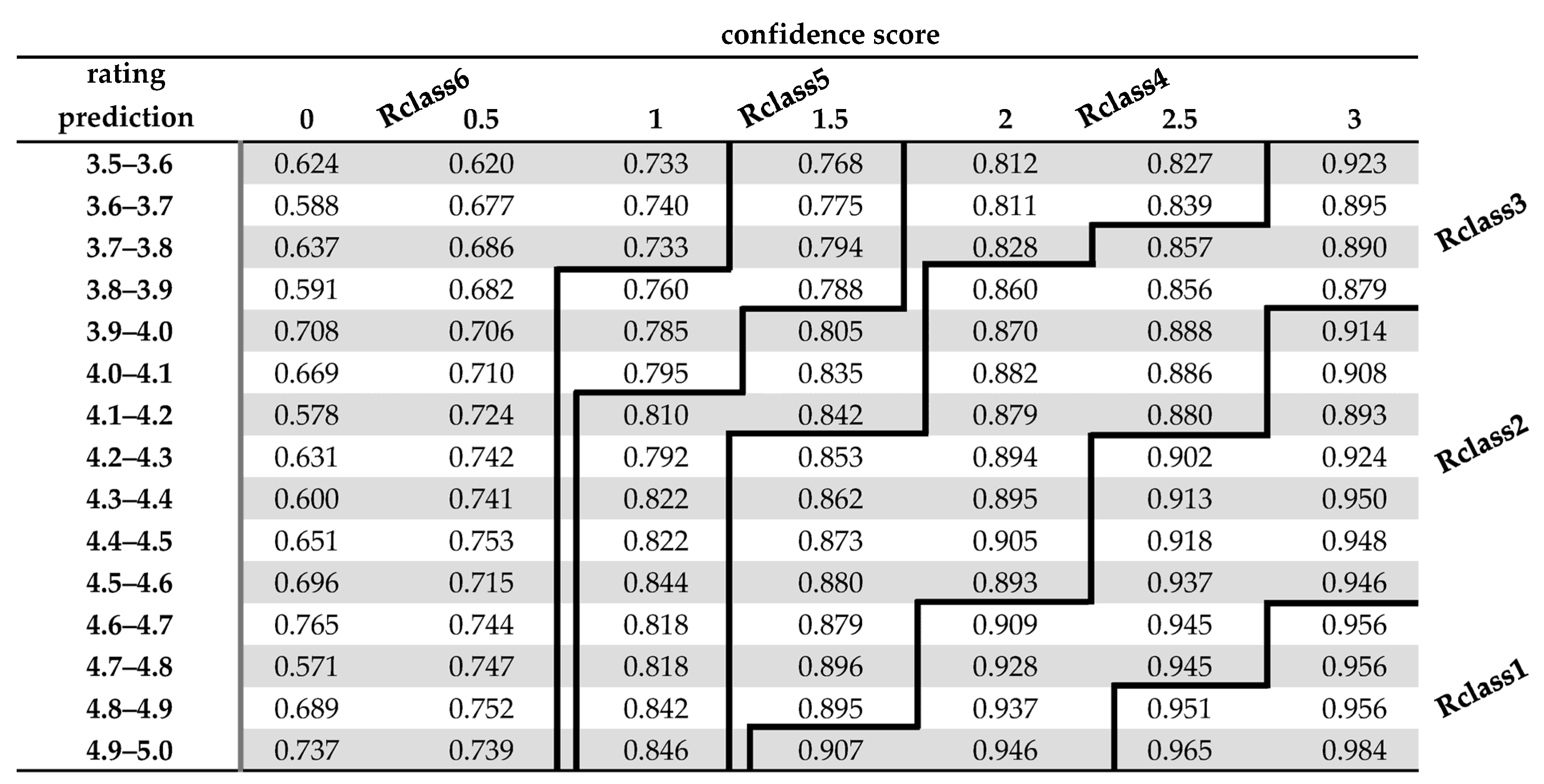
• Reliability Class 1 (Rclass1): it contains the rating predictions where (CSC = 3.0 AND RPV ≥ 4.6) OR (CSC = 2.5 AND RPV ≥ 4.8);
• Reliability Class 2 (Rclass2): it contains the rating predictions which do not already belong to RClass1 and where (CSC = 3.0 AND RPV ≥ 3.9) OR (CSC = 2.5 AND RPV ≥ 4.2) OR (CSC = 2.0 AND RPV ≥ 4.6) OR (CSC = 1.5 AND RPV ≥ 4.9);
• Reliability Class 3 (Rclass3): it contains the rating predictions which do not already belong to RClass1 or RClass2 and where (CSC = 3.0 AND RPV ≥ 3.5) OR (CSC = 2.5 AND RPV ≥ 3.7) OR (CSC = 2.0 AND RPV ≥ 3.8) OR (CSC = 1.5 AND RPV ≥ 4.2);
• Reliability Class 4 (Rclass4): it contains the rating predictions which do not already belong to RClass1, RClass2, or RClass3 and where (CSC = 2.5 AND RPV ≥ 3.5) OR (CSC = 2.0 AND RPV ≥ 3.5) OR (CSC = 1.5 AND RPV ≥ 3.9) OR (CSC = 1.0 AND RPV ≥ 4.1);
• Reliability Class 5 (Rclass5): it contains the rating predictions which do not already belong to RClass1, RClass2, RClass3, or RClass4 and where (CSC = 1.5 AND RPV ≥ 3.5) OR (CSC = 1.0 AND RPV ≥ 3.8);
• Reliability Class 6 (Rclass6): the rest of the rating predictions with RPV ≥ 3.5 (which is the typical threshold used by CF RecSys algorithms for a prediction to be considered in the recommendation formulation phase).

5.2. The Proposed Algorithm

The proposed CF algorithm modifies the typical recommendation formulation procedure to exploit the reliability class concept in order to generate more successful recommendations. In more detail, the proposed algorithm consists of the following three steps:

• The algorithm computes the RPV and CSC for every item prediction;
• The rating predictions with RPV ≥ 3.5 are classified into one of the six reliability classes, as defined above;
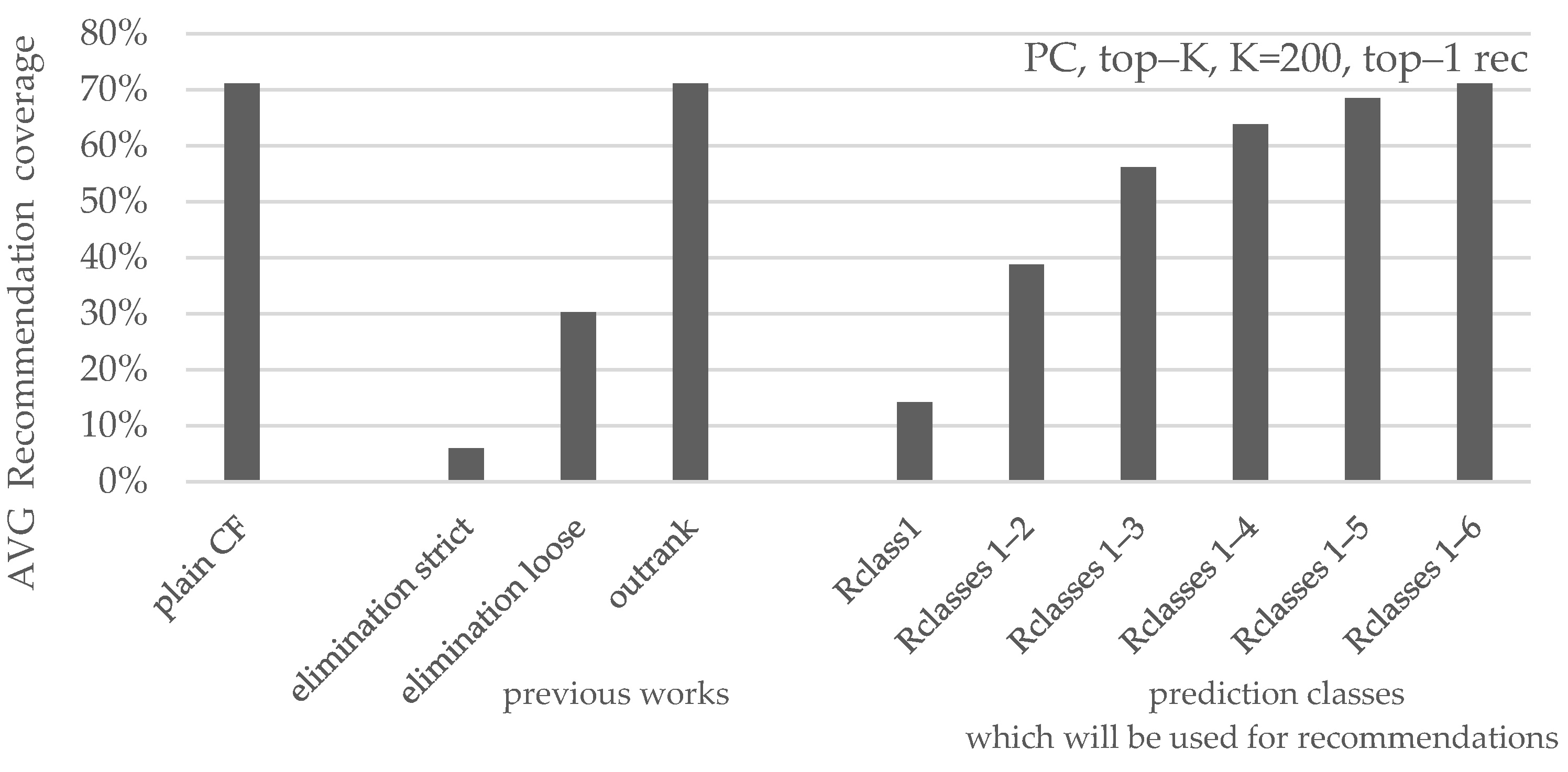
• For each user, the proposed algorithm begins to select items with predictions that belong to Rclass1. If they do not suffice, the items with predictions that belong to Rclass2 are selected for recommendation, and so on. If more than one item exists in the same class, based on the results shown in the previous subsection, firstly the CSC and secondly the RPV are used as tie-breakers.

In the next section, the proposed algorithm is experimentally evaluated, in terms of recommendation accuracy.

6. Experimental Evaluation

This section presents the experiments designed to assess the recommendation accuracy of the proposed algorithm. More specifically, we use the remaining six datasets from Table 1 (i.e., the Amazon Videogames, the Amazon Digital Music, the CiaoDVD, the Epinions, the MovieLens 100 K old, and the MovieLens 1 M), to ensure that the data used for the tuning of the algorithm are not utilized in the performance evaluation phase, ensuring the absence of bias.

Table 4. Average recommendation precision of the six reliability classes.

Class	Amazon Videogames	Amazon Digital Music	CiaoDVD	Epinions	MovieLens 100 K	MovieLens 1 M	AVG
Rclass1	98%	99%	96%	96%	97%	93%	97%
Rclass2	93%	97%	91%	91%	92%	92%	93%
Rclass3	85%	91%	86%	85%	88%	89%	87%
Rclass4	81%	87%	79%	81%	84%	87%	83%
Rclass5	76%	82%	74%	74%	76%	82%	78%
Rclass6	67%	74%	68%	68%	65%	68%	68%

depicts the recommendation precision (in percentage form) of the six reliability classes proposed in this work, for each of the six datasets, when the PC vicinity metric and TOP-K NN selection method with K = 200 are applied.

Table 5. Average actual rating value of the six reliability classes.

Class	Amazon Videogames	Amazon Digital Music	CiaoDVD	Epinions	MovieLens 100 K	MovieLens 1 M	AVG
Rclass1	4.87	4.94	4.75	4.75	4.72	4.67	4.78
Rclass2	4.69	4.84	4.51	4.54	4.58	4.57	4.62
Rclass3	4.40	4.48	4.31	4.33	4.38	4.45	4.39
Rclass4	4.26	4.28	4.14	4.18	4.25	4.37	4.25
Rclass5	4.10	4.13	4.04	3.98	4.01	4.21	4.08
Rclass6	3.81	3.97	3.79	3.77	3.77	3.85	3.83

depicts the average actual rating value of the recommendations under the same settings. Similar results are observed for all the rating prediction parameters tested (i.e., setting K = 500, using the CT NN selection method—both with thresholds 0.0 and 0.5—and using the CS user vicinity metric). These results can be found in

Table A1. Aggregated results of the mean recommendation precision of the six reliability classes, under different settings.

	Amazon Videogames	Amazon Digital Music	CiaoDVD	Epinions	MovieLens 100 K	MovieLens 1 M
PC, K = 200
Rclass1	98%	99%	96%	96%	97%	93%
Rclass2	93%	97%	92%	92%	92%	92%
Rclass3	84%	90%	86%	84%	87%	89%
Rclass4	81%	87%	79%	81%	84%	87%
Rclass5	76%	82%	76%	74%	76%	82%
Rclass6	67%	74%	66%	68%	65%	68%
PC, K = 500
Rclass1	97%	99%	97%	96%	97%	95%
Rclass2	93%	98%	90%	90%	92%	93%
Rclass3	85%	90%	84%	85%	86%	89%
Rclass4	81%	86%	79%	80%	81%	88%
Rclass5	75%	82%	74%	74%	74%	81%
Rclass6	68%	75%	65%	69%	64%	70%
PC, CT = 0.0
Rclass1	97%	99%	97%	96%	96%	96%
Rclass2	93%	98%	92%	91%	93%	93%
Rclass3	85%	91%	86%	84%	87%	85%
Rclass4	80%	87%	80%	80%	81%	77%
Rclass5	74%	82%	74%	72%	73%	72%
Rclass6	68%	74%	68%	70%	64%	61%
PC, CT = 0.5
Rclass1	97%	99%	97%	96%	93%	96%
Rclass2	93%	97%	92%	92%	94%	93%
Rclass3	85%	92%	85%	84%	88%	86%
Rclass4	81%	87%	81%	80%	86%	82%
Rclass5	75%	82%	76%	72%	77%	74%
Rclass6	68%	74%	68%	70%	67%	66%
CS, K = 200
Rclass1	97%	99%	96%	96%	94%	93%
Rclass2	93%	98%	91%	91%	94%	93%
Rclass3	85%	91%	85%	84%	88%	89%
Rclass4	81%	86%	80%	81%	86%	87%
Rclass5	76%	83%	76%	74%	79%	83%
Rclass6	67%	73%	70%	69%	66%	69%
CS, K = 500
Rclass1	97%	99%	96%	96%	96%	94%
Rclass2	93%	98%	91%	91%	93%	92%
Rclass3	84%	91%	84%	84%	85%	90%
Rclass4	80%	86%	81%	80%	83%	88%
Rclass5	75%	82%	75%	73%	75%	83%
Rclass6	67%	74%	68%	69%	65%	70%
CS, CT = 0.0
Rclass1	97%	99%	96%	96%	96%	96%
Rclass2	92%	98%	91%	91%	91%	91%
Rclass3	84%	91%	85%	84%	84%	84%
Rclass4	79%	85%	79%	79%	79%	78%
Rclass5	73%	81%	73%	72%	72%	72%
Rclass6	67%	73%	68%	71%	63%	61%
CS, CT = 0.5
Rclass1	97%	99%	96%	96%	95%	96%
Rclass2	93%	97%	90%	91%	92%	92%
Rclass3	84%	90%	85%	84%	84%	84%
Rclass4	79%	85%	79%	79%	79%	78%
Rclass5	73%	81%	73%	72%	73%	72%
Rclass6	67%	73%	68%	71%	67%	61%

and

Table A2. Aggregated results of the mean actual rating value of the recommendations of the reliability classes, under different settings.

	Amazon Videogames	Amazon Digital Music	CiaoDVD	Epinions	MovieLens 100 K	MovieLens 1 M
PC, K = 200
Rclass1	4.87	4.94	4.75	4.75	4.72	4.67
Rclass2	4.69	4.85	4.51	4.55	4.58	4.59
Rclass3	4.39	4.48	4.30	4.32	4.37	4.43
Rclass4	4.26	4.28	4.14	4.18	4.25	4.37
Rclass5	4.1	4.13	4.04	3.98	4.01	4.21
Rclass6	3.81	3.97	3.79	3.77	3.77	3.85
PC, K = 500
Rclass1	4.87	4.93	4.76	4.75	4.67	4.71
Rclass2	4.67	4.82	4.47	4.53	4.57	4.61
Rclass3	4.38	4.45	4.27	4.29	4.31	4.45
Rclass4	4.25	4.25	4.11	4.15	4.17	4.38
Rclass5	4.06	4.12	3.99	3.95	3.96	4.17
Rclass6	3.83	3.97	3.76	3.80	3.74	3.88
PC, CT = 0.0
Rclass1	4.87	4.94	4.77	4.75	4.65	4.72
Rclass2	4.69	4.84	4.54	4.52	4.58	4.53
Rclass3	4.39	4.46	4.29	4.28	4.31	4.31
Rclass4	4.22	4.26	4.12	4.11	4.14	4.05
Rclass5	4.04	4.15	3.98	3.90	3.94	3.92
Rclass6	3.84	3.96	3.80	3.84	3.72	3.67
PC, CT = 0.5
Rclass1	4.87	4.94	4.77	4.75	4.59	4.74
Rclass2	4.71	4.83	4.55	4.53	4.56	4.55
Rclass3	4.40	4.48	4.31	4.29	4.37	4.34
Rclass4	4.24	4.27	4.16	4.12	4.31	4.17
Rclass5	4.06	4.14	4.02	3.90	4.02	3.97
Rclass6	3.84	3.95	3.81	3.83	3.82	3.78
CS, K = 200
Rclass1	4.87	4.94	4.73	4.74	4.61	4.68
Rclass2	4.71	4.85	4.52	4.54	4.60	4.56
Rclass3	4.39	4.47	4.29	4.31	4.38	4.44
Rclass4	4.24	4.26	4.16	4.18	4.32	4.36
Rclass5	4.08	4.15	4.04	3.97	4.08	4.25
Rclass6	3.8	3.96	3.84	3.8	3.8	3.86
CS, K = 500
Rclass1	4.87	4.93	4.73	4.74	4.63	4.69
Rclass2	4.68	4.84	4.52	4.53	4.57	4.60
Rclass3	4.39	4.44	4.29	4.29	4.33	4.46
Rclass4	4.21	4.24	4.15	4.15	4.21	4.38
Rclass5	4.06	4.14	4	3.95	3.99	4.24
Rclass6	3.81	3.99	3.81	3.8	3.76	3.87
CS, CT = 0.0
Rclass1	4.86	4.93	4.74	4.74	4.66	4.72
Rclass2	4.67	4.83	4.50	4.53	4.54	4.49
Rclass3	4.35	4.42	4.29	4.28	4.28	4.28
Rclass4	4.18	4.24	4.11	4.11	4.12	4.07
Rclass5	4.01	4.14	3.95	3.90	3.92	3.91
Rclass6	3.83	3.97	3.80	3.85	3.70	3.66
CS, CT = 0.5
Rclass1	4.86	4.93	4.74	4.74	4.63	4.71
Rclass2	4.66	4.83	4.51	4.53	4.52	4.51
Rclass3	4.36	4.44	4.28	4.28	4.27	4.26
Rclass4	4.18	4.24	4.11	4.11	4.08	4.06
Rclass5	4.01	4.14	3.95	3.90	3.91	3.90
Rclass6	3.83	3.97	3.80	3.85	3.66	3.66

in Appendix A.

Based on these findings, if the CF RecSys is only able to select predictions from Rclass1 for recommendations, the recommendation precision is, on average, 97%. If predictions from Rclass2 are also recommended (i.e., the predictions that belong to Rclass1 do not suffice), the recommendation precision is, on average, 94%. In plain CF, if in the same six datasets the RecSys only recommends items with rating predictions in the range [4.75, 5] (which are considered excellent prediction values), the respective recommendation precision is measured as 90%, which is lower than the recommendation precision of both Rclass1 and Rclass2 introduced in this paper. The respective average real rating values are 4.78/5 (for Rclass1), 4.62/5 (for Rclass2), and 4.53 (for RPV ≥ 4.75).

In the next set of experiments, the proposed algorithm, which considers both the RPVs and their confidence factors, is compared to works that also take into account the aforementioned two CF prediction confidence factors, and more specifically, the work in [28] and the work in [29].

In more detail, the algorithm proposed in [28] prevents rating predictions with low prediction confidence factor values, and hence low certainty, from becoming recommendations. When applying this algorithm, we can either use the strict or the loose threshold confidence factor values (c.f. Section 3.2). When using the strict threshold values, we achieve higher recommendation success but very low recommendation coverage. When we use the loose threshold values, we achieve higher recommendation coverage but lower recommendation success. In the experiments that follow, we will use both alternatives for comprehensiveness; the algorithm utilizing strict thresholds will be termed “elimination strict” and the algorithm utilizing loose thresholds will be referred to as “elimination loose”. On the other hand, the work in [29] introduces a CF recommendation algorithm that allows for rating predictions with higher confidence factor values to outrank predictions with higher value but lower confidence factor values; this algorithm will be termed “outrank”.

Figure 5 depicts the mean recommendation coverage when recommending one item to each user and employing the Pearson Correlation similarity method and the KNN technique, with K = 200. As we mentioned above, the algorithm proposed in [28], when applying the strict thresholds (termed “elimination strict”), achieves an extremely low recommendation coverage. That is, it can recommend one item to only 5.9% of the users, on average. Furthermore, out of the six datasets tested, it was found that for one dataset (MovieLens 100 K) the recommendation coverage was 0%, and for another dataset (CiaoDVD) the recommendation coverage was 1.3% (i.e., this algorithm, with the strict thresholds, is able to recommend an item to less than 250 users out of the 17.6 K users of the dataset). Therefore, it was excluded from the next experiments. In this experiment, we can observe that, when solely using rating predictions which are classified in Rclass1 as recommendations, the coverage is relatively low (nevertheless, larger than the one the “elimination strict” achieves). However, when we include more classes in the recommendation formulation, the coverage quickly increases. For example, when we opt to use predictions from classes Rclass1, Rclass2, Rclass3, and Rclass4 (termed “Rclasses1–4”) as recommendations, the recommendation coverage is found to be 63.8%, which is comparable to the plain CF, which is found to be 71.1%. We can also observe that the algorithm proposed in [29] (termed “outrank”) and the algorithm proposed in this paper, when using all six Rclasses, do not lose recommendation coverage, since they do not prevent any rating predictions from becoming recommendations.

Figure 6 depicts the mean recommendation precision when recommending one item to each user and employing the Pearson Correlation similarity method and the KNN technique, with K = 200. We can observe that, when we only use predictions from Rclass1 as recommendations, their precision is extremely high, measured at 94.9%. As we add predictions classified in lower classes, the average recommendation precision decreases (from 91.1% for Rclasses1–2 to 86% for Rclasses1–6), as expected.

Figure 7 depicts the mean actual rating value of the recommendations when recommending one item to each user and employing the Pearson Correlation similarity method and the KNN technique, with K = 200. We can observe that the results are very similar to those of the recommendation precision metric (Figure 6). When we only use predictions from Rclass1 as recommendations, the average real rating value of the recommendation is 4.76/5. As we add predictions classified in lower classes, the average real rating value of the recommendations decreases (from 4.59/5 for Rclasses1–2 to 4.41/5 for Rclasses1–6), as expected.

A similar output is observed for all rating prediction parameters tested (i.e., setting K = 500, using the CT NN selection method with both thresholds 0.0 and 0.5, employing the CS user vicinity formula, and recommending three items—top-3 recs). These results can be found in

Table A3. Aggregated results of the proposed algorithm when recommending one item to each user (top-1), under different settings.

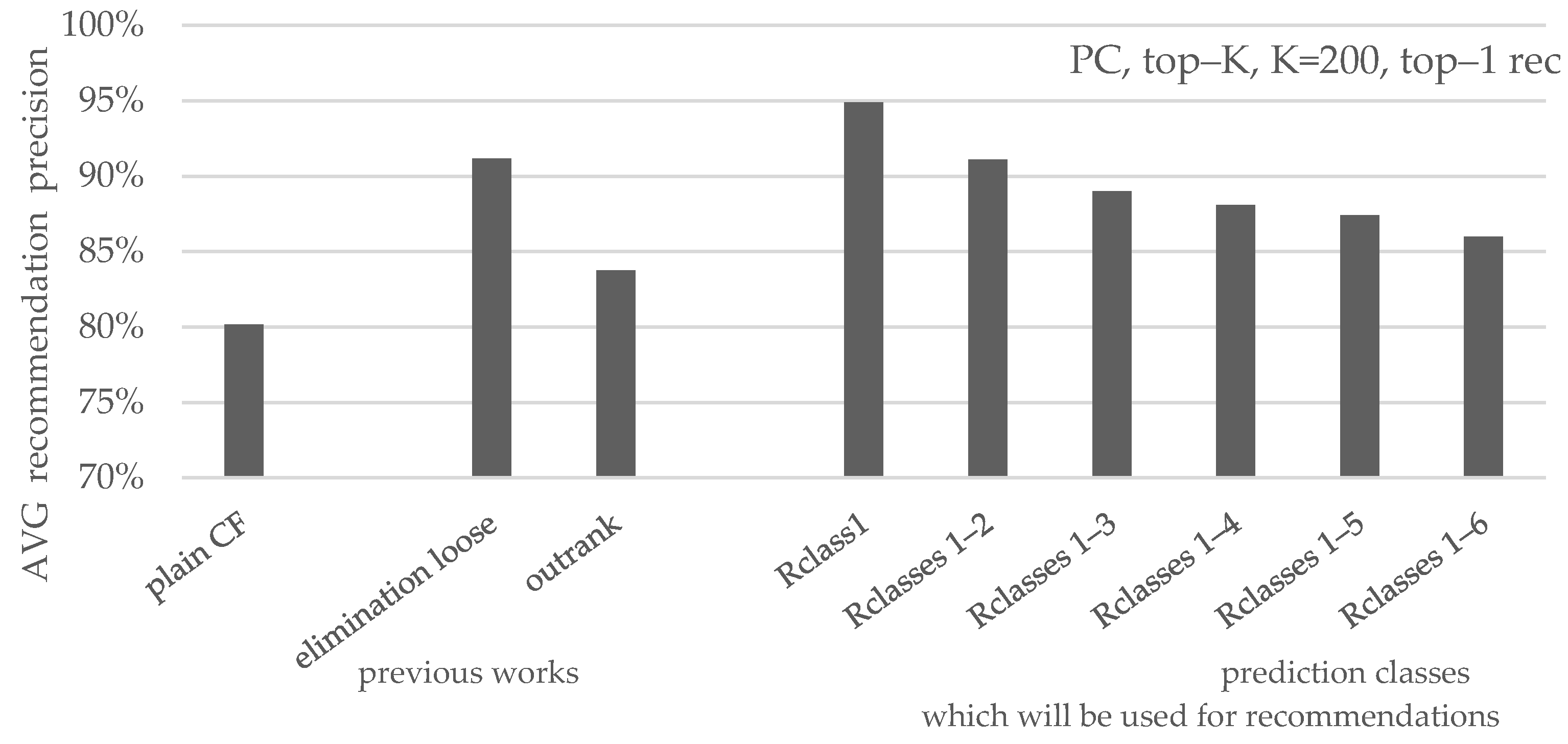
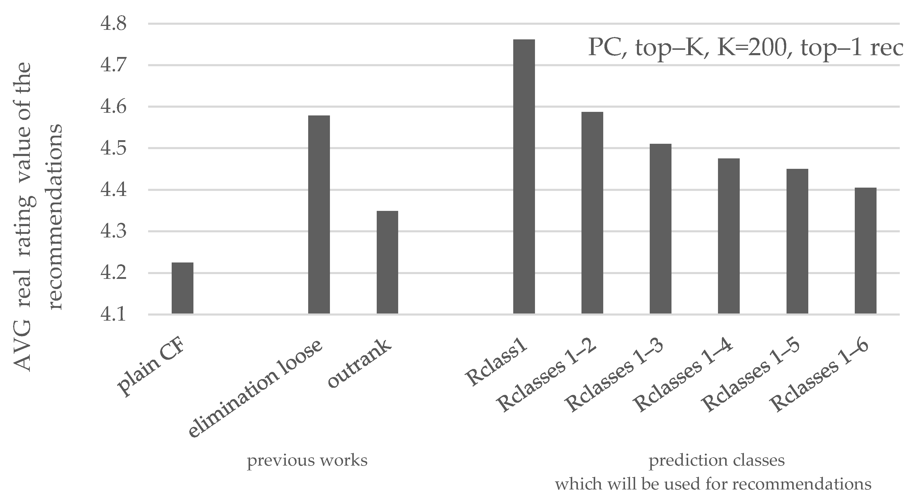
Setting/Metric	Rclass1	Rclasses1–2	Rclasses1–3	Rclasses1–4	Rclasses1–5	Rclasses1–6
PC, K = 200, top-1
avg. coverage	14.2%	38.8%	56.2%	63.8%	68.5%	71.1%
avg. precision	94.9%	91.0%	89.0%	88.1%	87.4%	86.0%
avg. real rating	4.76/5	4.60/5	4.50/5	4.48/5	4.45/5	4.41/5
PC, K = 500, top-1
avg. coverage	16.2%	40.7%	58.2%	64.7%	68.8%	71.4%
avg. precision	95.4%	91.3%	89.6%	88.4%	87.6%	86.5%
avg. real rating	4.77/5	4.59/5	4.51/5	4.48/5	4.46/5	4.42/5
PC, CT = 0.0, top-1
avg. coverage	18.2%	43.7%	60.5%	66.5%	69.8%	72.1%
avg. precision	95.6%	92.1%	90.1%	89.1%	88.4%	87.4%
avg. real rating	4.78/5	4.62/5	4.54/5	4.51/5	4.48/5	4.45/5
PC, CT = 0.5, top-1
avg. coverage	17.7%	43.5%	60.5%	65.2%	69.5%	71.9%
avg. precision	95.4%	92.1%	90.2%	88.4%	87.5%	86.2%
avg. real rating	4.76/5	4.62/5	4.52/5	4.49/5	4.46/5	4.42/5
CS, K = 200, top-1
avg. coverage	17.8%	42.7%	60.4%	69.0%	74.8%	78.2%
avg. precision	94.1%	90.7%	88.6%	87.5%	86.6%	84.9%
avg. real rating	4.72/5	4.58/5	4.48/5	4.46/5	4.43/5	4.38/5
CS, K = 500, top-1
avg. coverage	19.9%	44.8%	63.4%	70.8%	75.6%	78.3%
avg. precision	94.6%	91.1%	89.1%	88.0%	87.2%	85.9%
avg. real rating	4.75/5	4.61/5	4.49/5	4.47/5	4.45/5	4.41/5
CS, CT = 0.0, top-1
avg. coverage	22.9%	49.1%	66.7%	72.7%	76.2%	77.9%
avg. precision	95.1%	90.7%	88.9%	87.8%	87.0%	86.2%
avg. real rating	4.74/5	4.58/5	4.49/5	4.47/5	4.44/5	4.42/5
CS, CT = 0.5, top-1
avg. coverage	22.9%	49.3%	66.7%	72.7%	76.2%	77.9%
avg. precision	95.1%	90.8%	88.9%	87.7%	86.9%	86.1%
avg. real rating	4.75/5	4.62/5	4.49/5	4.47/5	4.44/5	4.41/5

and

Table A4. Aggregated results of the proposed algorithm when recommending three items to each user (top-3), under different settings.

Setting/Metric	Rclass1	Rclasses1–2	Rclasses1–3	Rclasses1–4	Rclasses1–5	Rclasses1–6
PC, K = 200, top-3
avg. coverage	5.8%	23.1%	37.9%	47.5%	55.6%	60.7%
avg. precision	95.6%	92.3%	90.3%	89.1%	87.9%	86.2%
avg. real rating	4.77/5	4.62/5	4.52/5	4.50/5	4.47/5	4.41/5
PC, K = 500, top-3
avg. coverage	7.5%	25.5%	41.6%	49.7%	56.3%	60.3%
avg. precision	95.6%	92.0%	90.2%	89.2%	88.1%	86.7%
avg. real rating	4.75/5	4.64/5	4.52/5	4.51/5	4.48/5	4.43/5
PC, CT = 0.0, top-3
avg. coverage	9.0%	29.1%	46.3%	53.6%	59.1%	62.2%
avg. precision	95.8%	92.9%	91.1%	89.9%	88.8%	87.7%
avg. real rating	4.76/5	4.67/5	4.57/5	4.53/5	4.50/5	4.46/5
PC, CT = 0.5, top-3
avg. coverage	8.5%	27.2%	42.4%	51.3%	57.9%	62.4%
avg. precision	95.5%	92.9%	90.8%	89.5%	88.3%	86.8%
avg. real rating	4.74/5	4.66/5	4.54/5	4.52/5	4.48/5	4.44/5
CS, K = 200, top-3
avg. coverage	7.2%	26.6%	40.9%	51.5%	61.0%	67.7%
avg. precision	94.8%	92.1%	90.1%	88.8%	87.4%	85.3%
avg. real rating	4.74/5	4.64/5	4.54/5	4.50/5	4.45/5	4.39/5
CS, K = 500, top-3
avg. coverage	9.4%	29.3%	45.4%	55.0%	63.2%	67.8%
avg. precision	95.2%	92.3%	90.3%	89.3%	88.0%	86.5%
avg. real rating	4.74/5	4.63/5	4.54/5	4.51/5	4.47/5	4.42/5
CS, CT = 0.0, top-3
avg. coverage	11.5%	33.2%	51.4%	59.1%	64.9%	67.7%
avg. precision	95.7%	92.1%	90.2%	89.0%	88.0%	87.1%
avg. real rating	4.75/5	4.65/5	4.52/5	4.50/5	4.47/5	4.44/5
CS, CT = 0.5, top-3
avg. coverage	11.5%	33.1%	51.5%	59.1%	65.0%	67.7%
avg. precision	95.7%	92.1%	90.1%	89.0%	87.9%	87.1%
avg. real rating	4.75/5	4.64/5	4.52/5	4.50/5	4.47/5	4.44/5

, in Appendix A.

7. Discussion

As demonstrated in the previous section, the experimental evaluation shows that the proposed algorithm, which is based on the novel concept of the reliability classes, is able to upgrade the recommendation accuracy in CF. Furthermore, the presented algorithm gives the RecSys administrator the ability to adjust the level of recommendation accuracy and/or coverage they need. More specifically, the RecSys administrator can choose between six alternatives of higher–lower recommendation coverage and recommendation accuracy and quality. For example, for datasets that reach higher initial recommendation coverage (for instance, when the plain CF algorithm achieves a recommendation coverage > 90%), the administrator may choose to include predictions from, e.g., Rclasses1–2. Conversely, for very sparse datasets (where the initial recommendation coverage is, for example, <30%) the administrator may choose to include predictions from Rclasses1–5.

Furthermore, we need to focus on two interesting cases to highlight the efficacy of the proposed algorithm.

The first case is the comparison between the algorithm presented in [28], termed “elimination loose”, and the case of Rclasses1–2 of the proposed algorithm, which recommends items with predictions classified in either Rclass1 (primarily) or Rclass2. We can notice that the algorithm proposed in this study shows equal recommendation accuracy to the “elimination loose” alternative of the algorithm presented in [28] (91.1% precision and 4.59/5 actual rating of recommendations, versus 91.2% and 4.58/5, respectively). Nonetheless, its recommendation coverage clearly surpasses the “elimination loose” alternative of the algorithm presented in [28] by 8.5% in absolute magnitude, which corresponds to an increase of 28%.

The second case is a comparison between the algorithm presented in [29], termed “outrank”, and the case of Rclasses1–6 of the proposed algorithm, which recommends items with predictions classified primarily in Rclass1, and then, in the absence of this, proceeds to Rclass2, etc., until Rclass6. Both these algorithms share the same recommendation coverage, equal to the coverage of the plain CF algorithm (since neither of them eliminates any predictions). However, the algorithm introduced in this work achieves both higher average recommendation precision (86.0% versus 83.8% for the algorithm presented in [29] and 80.2% for the plain CF) and average actual rating of recommendations (4.41/5 versus 4.35/5 for the algorithm presented in [29] and 4.23/5 for the plain CF) and therefore higher recommendation quality.

As a result, we can conclude that the algorithm presented in this work exhibits higher performance than both the algorithms presented in [28,29].

It is worth noting that, recently, rating prediction reliability has been considered in conjunction with deep learning models. More specifically, ref. [46] presents an extension of the Neural CF (NCF) method [47], which computes both rating predictions and their associated reliabilities, and then uses reliabilities in the recommendation formulation stage. The method proposed in [46] supersedes the plain NCF in terms of classification but lags behind the NCF in terms of the regression method. According to the authors, the computation and use of reliability indicators can be used for the detection of shilling attacks, promoting recommendation explainability, or within navigational tools to outline user and item dependencies. On the contrary, the method proposed in this paper achieves considerable improvements compared to the baselines. In our future work, we plan to use the prediction reliability factors in conjunction with machine learning models.

Deep learning approaches have also been employed for generic recommendation formulation without considering reliability aspects. The work in [48] presents a movie RecSys based on LightGCN [16] which models movie rating information as graphs and formulates recommendations by predicting user–movie edges on the graph. The evaluation presented in [48] indicates that the method proposed therein can achieve recommendation precision equal to 0.91 when applied to the MovieLens 1 M dataset. The algorithm proposed in this paper exhibits superior performance with the same dataset, achieving precision of up to 96% when recommendations are drawn only from Rclass1 and 92% when recommendations are drawn from either Rclass1 or Rclass2, and thus enhancing recommendation diversity.

The work in [49] uses graph embedding to model user behavior and proceeds with identifying users that are similar to the target user by applying decision trees, fuzzy rules, and ensemble learning. Once similar users are identified, a heterogeneous knowledge graph is constructed using the embedding vectors, and the graph is exploited to generate recommendations. The approach is evaluated using the MovieLens 1 M dataset, achieving precision equal to 82%. The algorithm proposed in this paper outperforms the one presented in [49], by achieving precision of up to 96% with the same dataset.

The work in [50] employs the novel Transformer Model approach to formulate recommendations. More specifically, the algorithm proposed in [50] utilizes a textual information source and a utility matrix data source, initially processing each of them individually through deep learning models, in order to extract pertinent features. Subsequently, the two feature sets are fused through transformers to generate recommendations. The evaluation presented in [50] achieves recommendation precision equal to 67.16% when applied to the MovieLens dataset and 83.31% when applied to the Amazon VideoGames dataset. The algorithm proposed in this paper surpasses this performance level, achieving precision of up to 96% when applied to the MovieLens dataset and up to 98% when applied to the Amazon VideoGames dataset.

In this work, we based the computation of confidence factors solely on the user–item rating matrix. This ensures that confidence factor computation can be performed on all datasets, since many datasets include only this basic information. It is worth noting the following, however:

• The methodology presented in this paper for recommendation formulation can be used in conjunction with rating prediction approaches that consider additional factors, such as user demographics, item categories and characteristics, contextual information, social network graphs, etc. This applies both to memory-based and user-based techniques;
• The confidence factor computation procedure can itself be augmented to consider the abovementioned additional factors and/or to use different weights for the contributing features.

In our future work, we plan to explore both these research directions.

8. Conclusions and Future Work

In this work, we advance the state-of-the-art in CF RecSys research by (a) introducing the concept of recommendation reliability classes; (b) formulating a total ordering of these classes, which is associated with the utility of the rating predictions belonging to each class; and (c) presenting a CF recommendation algorithm that prioritizes the rating predictions which are classified in higher reliability class(es) when making its recommendations. This algorithm gives the RecSys administrator the ability to adjust the level of recommendation quality and/or coverage they need. Furthermore, the proposed algorithm relies exclusively on the essential CF data and is thus able to be applied to every CF RecSys database/dataset.

We substantiated the efficacy of the proposed algorithm through an extensive multi-parameter assessment process, employing (a) two user vicinity metrics, (b) two methods for NN selection, and (c) eight CF datasets from multiple sources, to ensure generalizability. The proposed algorithm was found to achieve high recommendation quality results, in terms of recommendation accuracy and coverage, while it was found to outperform related and contemporary algorithms ([28,29], both published in 2024).

In our future work, we plan to study and experiment on alternative rating prediction features. Furthermore, we plan to study and experiment on different reliability class thresholds for each user. We also aim to incorporate additional data sources, where possible—from user demographics and social relations to item characteristics and product categories—to further enhance the recommendation quality in CF. Finally, we will consider the use of reliability assessments in conjunction with machine learning models.

References

- Wang, D.; Yih, Y.; Ventresca, M. Improving Neighbor-Based Collaborative Filtering by Using a Hybrid Similarity Measurement. Expert Syst. Appl. 2020, 160, 113651. [Google Scholar] [CrossRef]
- Rosa, R.E.; Guimarães, F.A.; da Silva Mendonça, R.; de Lucena, V.F. Improving Prediction Accuracy in Neighborhood-Based Collaborative Filtering by Using Local Similarity. IEEE Access 2020, 8, 142795–142809. [Google Scholar] [CrossRef]
- Jain, G.; Mahara, T.; Tripathi, K.N. A Survey of Similarity Measures for Collaborative Filtering-Based Recommender System. In Soft Computing: Theories and Applications; Pant, M., Sharma, T.K., Verma, O.P., Singla, R., Sikander, A., Eds.; Advances in Intelligent Systems and Computing; Springer: Singapore, 2020; Volume 1053, pp. 343–352. ISBN 978-981-15-0750-2. [Google Scholar]
- Khojamli, H.; Razmara, J. Survey of Similarity Functions on Neighborhood-Based Collaborative Filtering. Expert Syst. Appl. 2021, 185, 115482. [Google Scholar] [CrossRef]
- Nguyen, L.V.; Vo, Q.-T.; Nguyen, T.-H. Adaptive KNN-Based Extended Collaborative Filtering Recommendation Services. Big Data Cogn. Comput. 2023, 7, 106. [Google Scholar] [CrossRef]
- Fkih, F. Similarity Measures for Collaborative Filtering-Based Recommender Systems: Review and Experimental Comparison. J. King Saud Univ. Comput. Inf. Sci. 2022, 34, 7645–7669. [Google Scholar] [CrossRef]
- Koren, Y.; Rendle, S.; Bell, R. Advances in Collaborative Filtering. In Recommender Systems Handbook; Ricci, F., Rokach, L., Shapira, B., Eds.; Springer: New York, NY, USA, 2022; pp. 91–142. ISBN 978-1-0716-2196-7. [Google Scholar]
- Wu, L.; He, X.; Wang, X.; Zhang, K.; Wang, M. A Survey on Accuracy-Oriented Neural Recommendation: From Collaborative Filtering to Information-Rich Recommendation. IEEE Trans. Knowl. Data Eng. 2022, 35, 4425–4445. [Google Scholar] [CrossRef]
- Margaris, D.; Vassilakis, C.; Spiliotopoulos, D. On Producing Accurate Rating Predictions in Sparse Collaborative Filtering Datasets. Information 2022, 13, 302. [Google Scholar] [CrossRef]
- Spiliotopoulos, D.; Margaris, D.; Vassilakis, C. On Exploiting Rating Prediction Accuracy Features in Dense Collaborative Filtering Datasets. Information 2022, 13, 428. [Google Scholar] [CrossRef]
- Liao, C.-L.; Lee, S.-J. A Clustering Based Approach to Improving the Efficiency of Collaborative Filtering Recommendation. Electron. Commer. Res. Appl. 2016, 18, 1–9. [Google Scholar] [CrossRef]
- Valdiviezo-Diaz, P.; Ortega, F.; Cobos, E.; Lara-Cabrera, R. A Collaborative Filtering Approach Based on Naïve Bayes Classifier. IEEE Access 2019, 7, 108581–108592. [Google Scholar] [CrossRef]
- Margaris, D.; Vassilakis, C. Improving Collaborative Filtering’s Rating Prediction Quality in Dense Datasets, by Pruning Old Ratings. In Proceedings of the 2017 IEEE Symposium on Computers and Communications (ISCC), Heraklion, Greece, 3–6 July 2017; IEEE: Heraklion, Greece, 2017; pp. 1168–1174. [Google Scholar]
- Neysiani, B.S.; Soltani, N.; Mofidi, R.; Nadimi-Shahraki, M.H. Improve Performance of Association Rule-Based Collaborative Filtering Recommendation Systems Using Genetic Algorithm. Int. J. Inf. Technol. Comput. Sci. 2019, 11, 48–55. [Google Scholar] [CrossRef]
- Thakkar, P.; Varma, K.; Ukani, V.; Mankad, S.; Tanwar, S. Combining User-Based and Item-Based Collaborative Filtering Using Machine Learning. In Information and Communication Technology for Intelligent Systems; Satapathy, S.C., Joshi, A., Eds.; Smart Innovation, Systems and Technologies; Springer: Singapore, 2019; Volume 107, pp. 173–180. ISBN 978-981-13-1746-0. [Google Scholar]
- He, X.; Deng, K.; Wang, X.; Li, Y.; Zhang, Y.; Wang, M. LightGCN: Simplifying and Powering Graph Convolution Network for Recommendation. In Proceedings of the 43rd International ACM SIGIR Conference on Research and Development in Information Retrieval, Virtual Event, China, 25–30 July 2020; ACM: New York, NY, USA, 2020; pp. 639–648. [Google Scholar]
- Li, A.; Cheng, Z.; Liu, F.; Gao, Z.; Guan, W.; Peng, Y. Disentangled Graph Neural Networks for Session-Based Recommendation. IEEE Trans. Knowl. Data Eng. 2023, 35, 7870–7882. [Google Scholar] [CrossRef]
- Wei, Y.; Wang, X.; Li, Q.; Nie, L.; Li, Y.; Li, X.; Chua, T.-S. Contrastive Learning for Cold-Start Recommendation. In Proceedings of the 29th ACM International Conference on Multimedia, Virtual Event, China, 20–24 October 2021; ACM: New York, NY, USA, 2021; pp. 5382–5390. [Google Scholar]
- Yang, B.; Lei, Y.; Liu, J.; Li, W. Social Collaborative Filtering by Trust. IEEE Trans. Pattern Anal. Mach. Intell. 2017, 39, 1633–1647. [Google Scholar] [CrossRef] [PubMed]
- Wang, Y.; Deng, J.; Gao, J.; Zhang, P. A Hybrid User Similarity Model for Collaborative Filtering. Inf. Sci. 2017, 418–419, 102–118. [Google Scholar] [CrossRef]
- Islam, R.; Keya, K.N.; Zeng, Z.; Pan, S.; Foulds, J. Debiasing Career Recommendations with Neural Fair Collaborative Filtering. In Proceedings of the Web Conference 2021, Ljubljana, Slovenia, 19–23 April 2021; ACM: New York, NY, USA, 2021; pp. 3779–3790. [Google Scholar]
- Iwendi, C.; Ibeke, E.; Eggoni, H.; Velagala, S.; Srivastava, G. Pointer-Based Item-to-Item Collaborative Filtering Recommendation System Using a Machine Learning Model. Int. J. Inf. Technol. Decis. Mak. 2022, 21, 463–484. [Google Scholar] [CrossRef]
- Chen, G.; Zeng, F.; Zhang, J.; Lu, T.; Shen, J.; Shu, W. An Adaptive Trust Model Based on Recommendation Filtering Algorithm for the Internet of Things Systems. Comput. Netw. 2021, 190, 107952. [Google Scholar] [CrossRef]
- Chang, J.-L.; Li, H.; Bi, J.-W. Personalized Travel Recommendation: A Hybrid Method with Collaborative Filtering and Social Network Analysis. Curr. Issues Tour. 2022, 25, 2338–2356. [Google Scholar] [CrossRef]
- Vuong Nguyen, L.; Nguyen, T.; Jung, J.J.; Camacho, D. Extending Collaborative Filtering Recommendation Using Word Embedding: A Hybrid Approach. Concurr. Comput. Pract. Exp. 2023, 35, e6232. [Google Scholar] [CrossRef]
- Rohit; Sabitha, S.; Choudhury, T. Proposed Approach for Book Recommendation Based on User K-NN. In Advances in Computer and Computational Sciences; Bhatia, S.K., Mishra, K.K., Tiwari, S., Singh, V.K., Eds.; Advances in Intelligent Systems and Computing; Springer: Singapore, 2018; Volume 554, pp. 543–558. ISBN 978-981-10-3772-6. [Google Scholar]
- Shambour, Q. A Deep Learning Based Algorithm for Multi-Criteria Recommender Systems. Knowl. Based Syst. 2021, 211, 106545. [Google Scholar] [CrossRef]
- Margaris, D.; Sgardelis, K.; Spiliotopoulos, D.; Vassilakis, C. Exploiting Rating Prediction Certainty for Recommendation Formulation in Collaborative Filtering. Big Data Cogn. Comput. 2024, 8, 53. [Google Scholar] [CrossRef]
- Sgardelis, K.; Margaris, D.; Spiliotopoulos, D.; Vassilakis, C.; Ougiaroglou, S. Improving Recommendation Quality in Collaborative Filtering by Including Prediction Confidence Factors. In Proceedings of the 20th International Conference on Web Information Systems and Technologies, Porto, Portugal, 17–19 November 2024; SCITEPRESS—Science and Technology Publications: Setúbal, Portugal, 2024; pp. 372–379. [Google Scholar]
- Pugoy, R.A.; Kao, H.-Y. NEAR: Non-Supervised Explainability Architecture for Accurate Review-Based Collaborative Filtering. IEEE Trans. Knowl. Data Eng. 2022, 36, 750–765. [Google Scholar] [CrossRef]
- Ghasemi, N.; Momtazi, S. Neural Text Similarity of User Reviews for Improving Collaborative Filtering Recommender Systems. Electron. Commer. Res. Appl. 2021, 45, 101019. [Google Scholar] [CrossRef]
- Chen, Y.; Xie, T.; Chen, H.; Huang, X.; Cui, N.; Li, J. KGCF: Social Relationship-Aware Graph Collaborative Filtering for Recommendation. Inf. Sci. 2024, 680, 121102. [Google Scholar] [CrossRef]
- Lee, Y.-C. Application of Support Vector Machines to Corporate Credit Rating Prediction. Expert Syst. Appl. 2007, 33, 67–74. [Google Scholar] [CrossRef]
- Ni, J.; Li, J.; McAuley, J. Justifying Recommendations Using Distantly-Labeled Reviews and Fine-Grained Aspects. In Proceedings of the 2019 Conference on Empirical Methods in Natural Language Processing and the 9th International Joint Conference on Natural Language Processing (EMNLP-IJCNLP), Hong Kong, China, 3–7 November 2019; Association for Computational Linguistics: Stroudsburg, PA, USA, 2019; pp. 188–197. [Google Scholar]
- Guo, G.; Zhang, J.; Thalmann, D.; Yorke-Smith, N. ETAF: An Extended Trust Antecedents Framework for Trust Prediction. In Proceedings of the 2014 IEEE/ACM International Conference on Advances in Social Networks Analysis and Mining (ASONAM 2014), Beijing, China, 17–20 August 2014; IEEE: Beijing, China, 2014; pp. 540–547. [Google Scholar]
- Richardson, M.; Agrawal, R.; Domingos, P. Trust Management for the Semantic Web. In The Semantic Web—ISWC 2003; Fensel, D., Sycara, K., Mylopoulos, J., Eds.; Lecture Notes in Computer Science; Springer: Berlin, Heidelberg, 2003; Volume 2870, pp. 351–368. ISBN 978-3-540-20362-9. [Google Scholar]
- Harper, F.M.; Konstan, J.A. The MovieLens Datasets: History and Context. ACM Trans. Interact. Intell. Syst. 2016, 5, 1–19. [Google Scholar] [CrossRef]
- Krichene, W.; Rendle, S. On Sampled Metrics for Item Recommendation. In Proceedings of the 26th ACM SIGKDD International Conference on Knowledge Discovery & Data Mining, Virtual Event, CA, USA, 6–10 July 2020; ACM: New York, NY, USA, 2020; pp. 1748–1757. [Google Scholar]
- Chin, J.Y.; Chen, Y.; Cong, G. The Datasets Dilemma: How Much Do We Really Know About Recommendation Datasets? In Proceedings of the Fifteenth ACM International Conference on Web Search and Data Mining, Virtual Event, AZ, USA, 21–25 February 2022; ACM: New York, NY, USA, 2022; pp. 141–149. [Google Scholar]
- Margaris, D.; Vassilakis, C.; Spiliotopoulos, D. What Makes a Review a Reliable Rating in Recommender Systems? Inf. Process. Manag. 2020, 57, 102304. [Google Scholar] [CrossRef]
- Trattner, C.; Said, A.; Boratto, L.; Felfernig, A. Evaluating Group Recommender Systems. In Group Recommender Systems; Felfernig, A., Boratto, L., Stettinger, M., Tkalčič, M., Eds.; Signals and Communication Technology; Springer Nature: Cham, Switzerland, 2024; pp. 63–75. ISBN 978-3-031-44942-0. [Google Scholar]
- Felfernig, A.; Boratto, L.; Stettinger, M.; Tkalčič, M. Evaluating Group Recommender Systems. In Group Recommender Systems; Springer Briefs in Electrical and Computer Engineering; Springer: Cham, Switzerland, 2018; pp. 59–71. [Google Scholar]
- Ackermann, M.R.; Blömer, J.; Kuntze, D.; Sohler, C. Analysis of Agglomerative Clustering. Algorithmica 2014, 69, 184–215. [Google Scholar] [CrossRef]
- Tokuda, E.K.; Comin, C.H.; Costa, L.D.F. Revisiting Agglomerative Clustering. Phys. A Stat. Mech. Appl. 2022, 585, 126433. [Google Scholar] [CrossRef]
- Xiao, J.; Lu, J.; Li, X. Davies Bouldin Index Based Hierarchical Initialization K-Means. Intell. Data Anal. 2017, 21, 1327–1338. [Google Scholar] [CrossRef]
- Bobadilla, J.; Gutiérrez, A.; Alonso, S.; González-Prieto, Á. Neural Collaborative Filtering Classification Model to Obtain Prediction Reliabilities. Int. J. Interact. Multimed. Artif. Intell. 2022, 7, 18. [Google Scholar] [CrossRef]
- He, X.; Liao, L.; Zhang, H.; Nie, L.; Hu, X.; Chua, T.-S. Neural Collaborative Filtering. In Proceedings of the 26th International Conference on World Wide Web, Perth, Australia, 3–7 April 2017; International World Wide Web Conferences Steering Committee: Geneva, Switzerland, 2017; pp. 173–182. [Google Scholar]
- Nesmaoui, R.; Louhichi, M.; Lazaar, M. A Collaborative Filtering Movies Recommendation System Based on Graph Neural Network. Procedia Comput. Sci. 2023, 220, 456–461. [Google Scholar] [CrossRef]
- Forouzandeh, S.; Berahmand, K.; Rostami, M. Presentation of a Recommender System with Ensemble Learning and Graph Embedding: A Case on MovieLens. Multimed. Tools Appl. 2021, 80, 7805–7832. [Google Scholar] [CrossRef]
- Ho, T.-L.; Le, A.-C.; Vu, D.-H. Multiview Fusion Using Transformer Model for Recommender Systems: Integrating the Utility Matrix and Textual Sources. Appl. Sci. 2023, 13, 6324. [Google Scholar] [CrossRef]