Impact on Classification Process Generated by Corrupted Features


Abstract
1. Introduction
2. Related Work
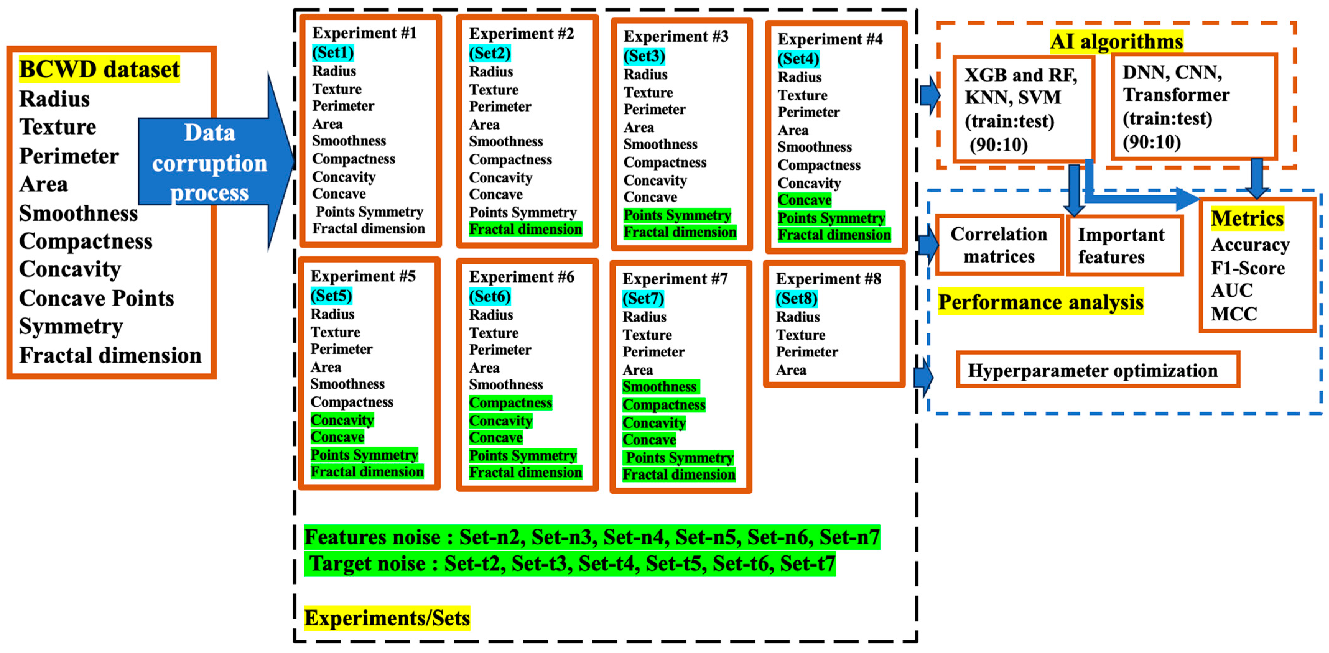
3. Proposed Methodology
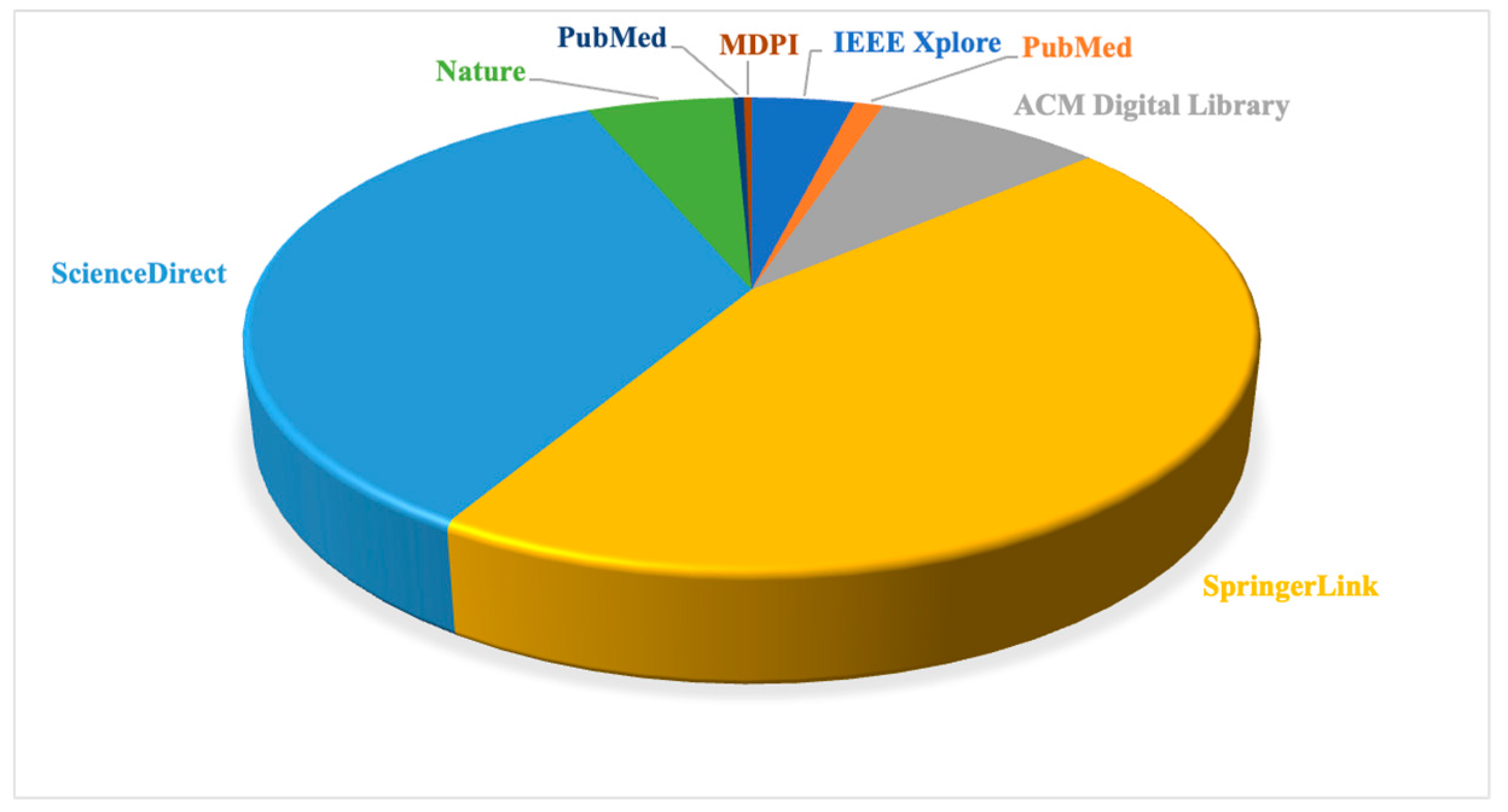
4. Information Sources and Search Strategy
5. Short Description of Artificial Intelligence Algorithms Used in Experiments
5.1. Machine Learning Algorithms
5.2. Deep Neural Network (DNN)
5.3. Convolutional Neural Network (CNN)
5.4. Transformer Neural Network (TNN)
6. Mathematical Approaches
6.1. Correlation Matrix
6.2. Confusion Matrix and Metrics
7. Results and Discussions
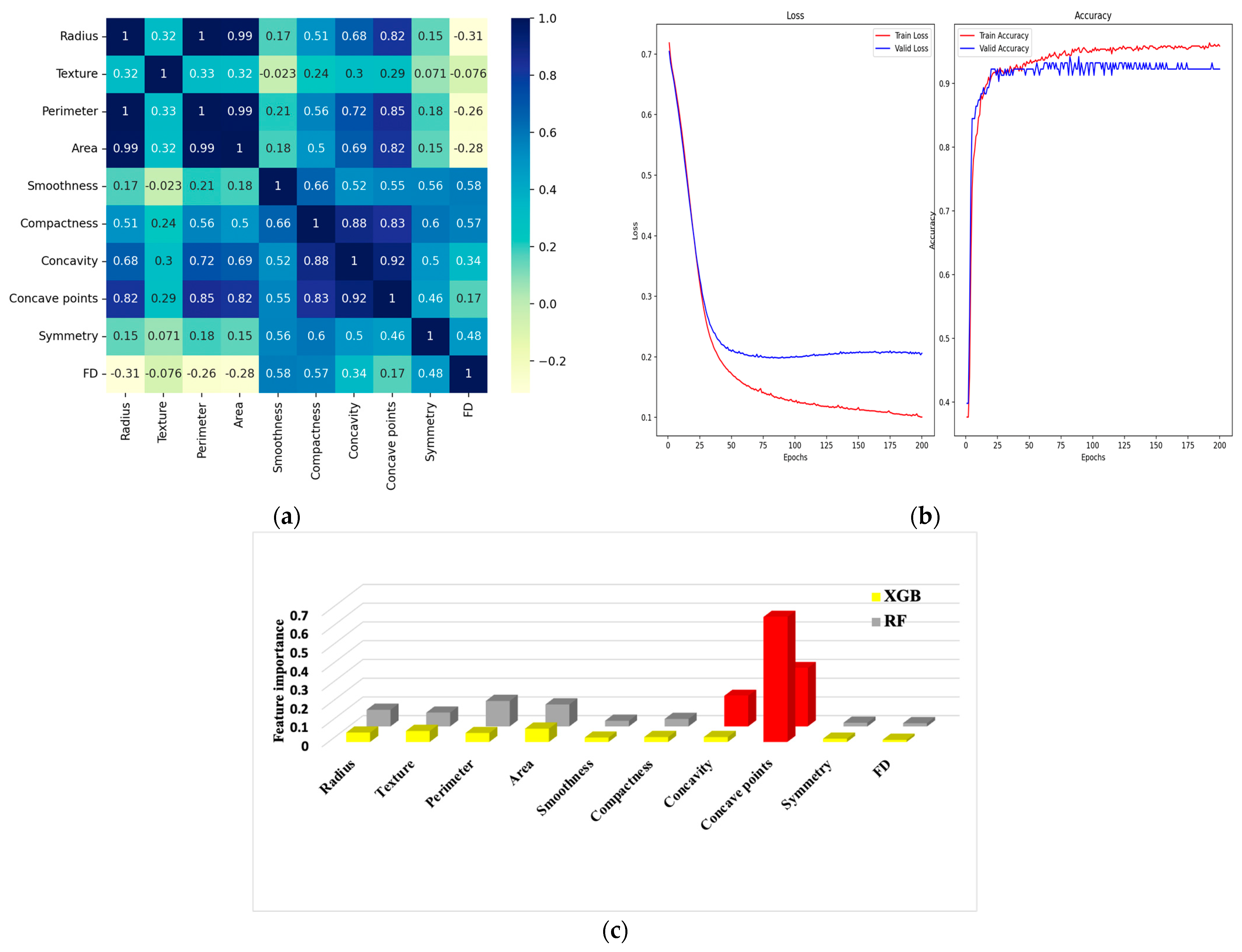
7.1. Experiment #1
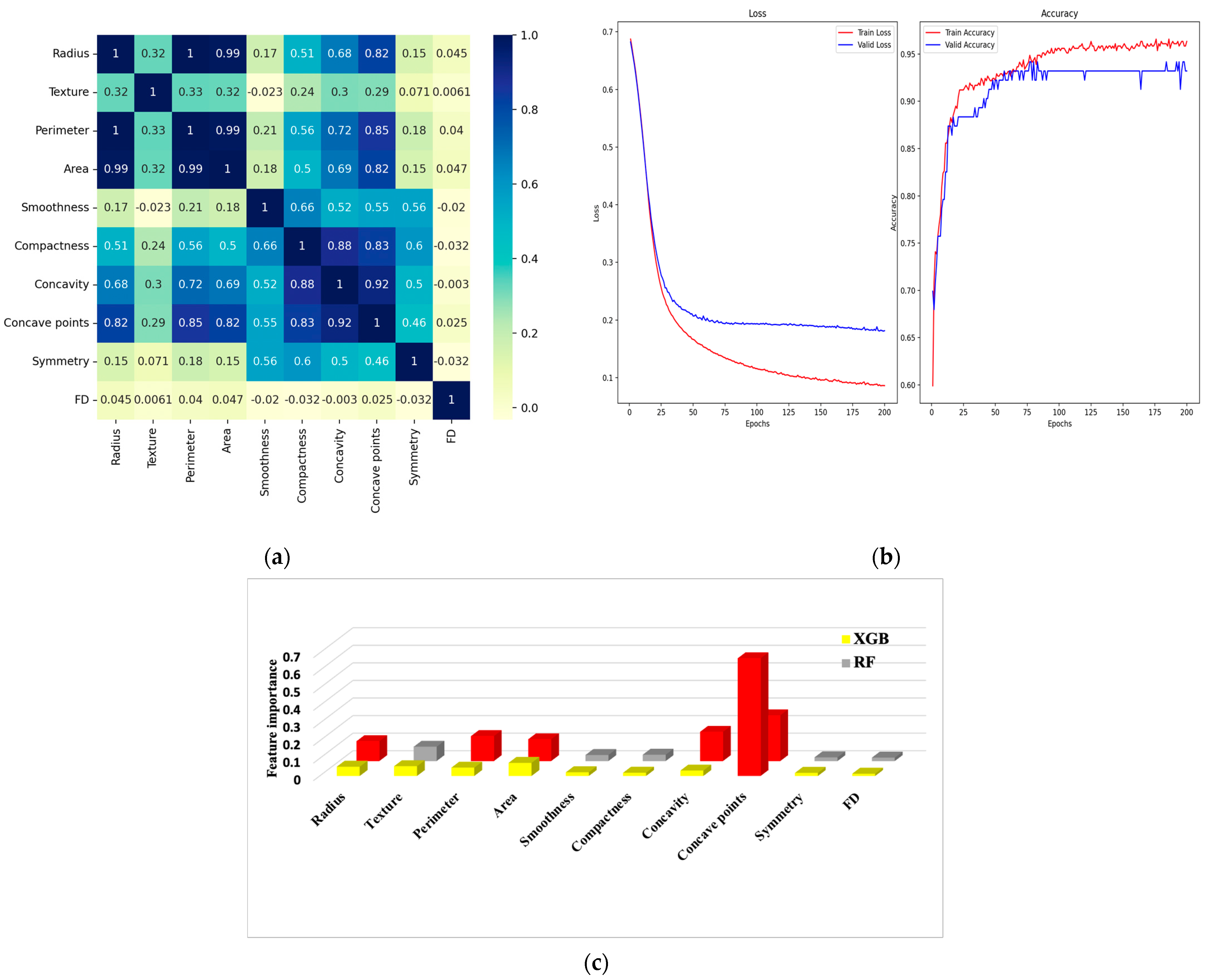
7.2. Experiment #2
7.3. Experiment #3
7.4. Experiment #4
7.5. Experiment #5
7.6. Experiment #6
7.7. Experiment #7
7.8. Experiment #8
7.9. Hyperparameters Optimization
7.9.1. DNN Hyperparameters Optimization
7.9.2. RF Hyperparameters Optimization
7.9.3. XGB Hyperparameters Optimization
7.9.4. SVM Hyperparameters Optimization
7.9.5. KNN Hyperparameters Optimization
7.9.6. CNN Hyperparameters Optimization
7.9.7. Transformer Hyperparameters Optimization
7.10. Discussion
8. Conclusions
Author Contributions
Funding
Data Availability Statement
Acknowledgments
Conflicts of Interest
References
- Pichugin, Y.A.; Malafeyev, O.A.; Rylow, D.; Zaitseva, I. A statistical method for corrupt agents detection. In AIP Conference Proceedings; AIP Publishing: Melville, NY, USA, 2018. [Google Scholar]
- Zhu, Z.; Dong, Z.; Liu, Y. Detecting corrupted labels without training a model to predict. In Proceedings of the 39th International Conference on Machine Learning, PMLR, Baltimore, MD, USA, 17–23 July 2022; pp. 27412–27427. [Google Scholar]
- Rankin, D.; Black, M.; Bond, R.; Wallace, J.; Mulvenna, M.; Epelde, G. Reliability of Supervised Machine Learning Using Synthetic Data in Health Care: Model to Preserve Privacy for Data Sharing. JMIR Med. Inform. 2020, 8, e18910. [Google Scholar] [CrossRef]
- Torfi, A.; Fox, E.A.; Reddy, C.K. Differentially private synthetic medical data generation using convolutional GANs. Inf. Sci. 2022, 586, 485–500. [Google Scholar] [CrossRef]
- Goncalves, A.; Ray, P.; Soper, B.; Stevens, J.; Coyle, L.; Sales, A.P. Generation and evaluation of synthetic patient data. BMC Med. Res. Methodol. 2020, 20, 108. [Google Scholar] [CrossRef]
- Banville, H.; Wood, S.U.; Aimone, C.; Engemann, D.A.; Gramfort, A. Robust learning from corrupted EEG with dynamic spatial filtering. NeuroImage 2022, 251, 118994. [Google Scholar] [CrossRef] [PubMed]
- Budach, L.; Feuerpfeil, M.; Ihde, N.; Nathansen, A.; Noack, N.; Patzlaff, H.; Harmouch, H.; Naumann, F. The Effects of Data Quality on Machine Learning Performance. arXiv 2022, arXiv:2207.14529. [Google Scholar]
- Wu, Z.; Rincon, D.; Luo, J.; Christofides, P.D. Machine learning modeling and predictive control of nonlinear processes using noisy data. AIChE J. 2021, 67, e17164. [Google Scholar] [CrossRef]
- Alhajeri, M.S.; Abdullah, F.; Wu, Z.; Christofides, P.D. Physics-informed machine learning modeling for predictive control using noisy data. Chem. Eng. Res. Des. 2022, 186, 34–49. [Google Scholar] [CrossRef]
- Lee, Y.; Barber, R.F. Binary classification with corrupted labels. Electron. J. Stat. 2022, 16, 1367–1392. [Google Scholar] [CrossRef]
- Feldman, S.; Einbinder, B.S.; Bates, S.; Angelopoulos, A.N.; Gendler, A.; Romano, Y. Conformal prediction is robust to dispersive label noise. In Proceedings of the Conformal and Probabilistic Prediction with Applications, Limassol, Cyprus, 13–15 September 2023; Volume 186, pp. 34–49. [Google Scholar]
- Hendrycks, D.; Mazeika, M.; Wilson, D.; Gimpel, K. Using trusted data to train deep networks on labels corrupted by severe noise Advances in Neural Information Processing Systems. Adv. Neural Inf. Process. Syst. 2018, 31, 10456–11046. [Google Scholar]
- Kadhim, R.R.; Kamil, M.Y. Comparison of breast cancer classification models on Wisconsin dataset. Int. J. Reconfigurable Embed. Syst. 2022, 2089, 4864. [Google Scholar] [CrossRef]
- Mohammad, W.; Teete, R.; Al-Aaraj, H.; Rubbai, Y.; Arabyat, M. Diagnosis of breast cancer pathology on the Wisconsin dataset with the help of data mining classification and clustering techniques. Appl. Bionics Biomech. 2022, 9, 6187275. [Google Scholar] [CrossRef] [PubMed]
- Abdulkareem, S.A.; Abdulkareem, Z.O. An evaluation of the Wisconsin breast cancer dataset using ensemble classifiers and RFE feature selection. Int. J. Sci. Basic Appl. Res. 2021, 55, 67–80. [Google Scholar]
- El-Shair, Z.A.; Sánchez-Pérez, L.A.; Rawashdeh, S.A. Comparative Study of Machine Learning Algorithms Using a Breast Cancer Dataset. In Proceedings of the 2020 IEEE International Conference on Electro Information Technology (EIT), Chicago, IL, USA, 31 July–1 August 2020; pp. 500–508. [Google Scholar]
- Sujon, M.A.H.; Mustafa, H. Comparative Study of Machine Learning Models on Multiple Breast Cancer Datasets. Int. J. Adv. Sci. Comput. Eng. 2023, 5, 15–24. [Google Scholar] [CrossRef]
- Hernández-Julio, Y.F.; Díaz-Pertuz, L.A.; Prieto-Guevara, M.J.; Barrios-Barrios, M.A.; Nieto-Bernal, W. Intelligent fuzzy system to predict the wisconsin breast cancer dataset. Int. J. Environ. Res. Public Health 2023, 20, 5103. [Google Scholar] [CrossRef]
- Jony, A.; Arnob, A.K. Deep Learning Paradigms for Breast Cancer Diagnosis: A Comparative Study on Wisconsin Diagnostic Dataset. Malays. J. Sci. Adv. Technol. 2024, 4, 109–117. [Google Scholar] [CrossRef]
- Mushtaq, Z.; Qureshi, M.F.; Abbass, M.J.; Al-Fakih, S.M.Q. Effective kernel-principal component analysis based approach for wisconsin breast cancer diagnosis. Electron. Lett. 2023, 59, e212706. [Google Scholar] [CrossRef]
- Street, W.N.; Wolberg, W.H.; Mangasarian, O.L. Nuclear feature extraction for breast tumor diagnosis. In Proceedings of the IS&T/SPIE 1993 International Symposium on Electronic Imaging: Science and Technology, San Jose, CA, USA, 31 January–5 February 1993; Volume 1905, pp. 861–870. [Google Scholar]
- Hu, J.; Szymczak, S. A review on longitudinal data analysis with random forest. Briefings Bioinform. 2023, 24, bbad002. [Google Scholar] [CrossRef] [PubMed]
- Tabacaru, G.; Moldovanu, S.; Răducan, E.; Barbu, M. A Robust Machine Learning Model for Diabetic Retinopathy Classification. J. Imaging 2024, 10, 8. [Google Scholar] [CrossRef] [PubMed]
- Damian, F.A.; Moldovanu, S.; Moraru, L. Melanoma detection using a random forest algorithm. In Proceedings of the 2022 E-Health and Bioengineering Conference (EHB), Iasi, Romania, 17–18 November 2022; IEEE: Piscataway, NJ, USA, 2022; pp. 1–4. [Google Scholar]
- Khan, M.S.; Nath, T.D.; Hossain, M.M.; Mukherjee, A.; Hasnath, H.B.; Meem, T.M.; Khan, U. Comparison of multiclass classification techniques using dry bean dataset. Int. J. Cogn. Comput. Eng. 2023, 4, 6–20. [Google Scholar]
- Bansal, M.; Goyal, A.; Choudhary, A. A comparative analysis of K-Nearest Neighbour, Genetic, Support Vector Machine, Decision Tree, and Long Short Term Memory algorithms in machine learning. Decis. Anal. J. 2022, 3, 10007. [Google Scholar]
- Oluleye, B.I.; Chan, D.W.; Antwi-Afari, P. Adopting Artificial Intelligence for enhancing the implementation of systemic circularity in the construction industry: A critical review. Sustain. Prod. Consum. 2022, 35, 509–524. [Google Scholar] [CrossRef]
- Trifan, L.S.; Moldovanu, S. Analyzing deep learning algorithms with statistical methods. Syst. Theory Control Comput. J. 2024, 4, 9–14. [Google Scholar] [CrossRef]
- LeCun, Y.; Bengio, Y.; Hinton, G. Deep learning. Nature 2015, 521, 436–444. [Google Scholar] [CrossRef] [PubMed]
- Vaswani, A.; Shazeer, N.; Parmar, N.; Uszkoreit, J.; Jones, L.; Gomez, A.N.; Kaiser, Ł.; Polosukhin, I. Attention is all you need. Adv. Neural Inf. Process. 2017. [Google Scholar]
- Starmans, M.P.; van derVoort, S.R.; Tovar, J.M.C.; Veenland, J.F.; Klein, S.; Niessen, W.J. Radiomics: Data mining using quantitative medical image features. In Handbook of Medical Image Computing and Computer Assisted Intervention; Elsevier: Amsterdam, The Netherlands, 2020; pp. 429–456. [Google Scholar]
- Baak, M.; Koopman, R.; Snoek, H.; Klous, S. A new correlation coefficient between categorical, ordinal and interval variables with pearson characteristics. Comput. Stat. Data Anal. 2020, 152, 107043. [Google Scholar] [CrossRef]
- Ratner, B. The correlation coefficient: Its values range between +1/−1, or do they? J. Target. Meas. Anal. Mark. 2009, 17, 139–142. [Google Scholar] [CrossRef]
- Chicco, D.; Tötsch, N.; Jurman, G. The Matthews correlation coefficient (MCC) is more re-liable than balanced accuracy, bookmaker informedness, and markedness in two-class confusion matrix evaluation. BioData Min. 2021, 14, 13. [Google Scholar] [CrossRef]


| Feature Dataset | Diagnosis | Radius | Texture | Perimeter | Area | Smoothness | Compactness | Concavity | Concave Points | Symmetry | FD |
|---|---|---|---|---|---|---|---|---|---|---|---|
| Set 1 | - | - | - | - | - | - | - | - | - | - | - |
| Set 2 | - | - | - | - | - | - | - | - | - | - | * |
| Set 3 | - | - | - | - | - | - | - | - | - | * | * |
| Set 4 | - | - | - | - | - | - | - | - | * | * | * |
| Set 5 | - | - | - | - | - | - | - | * | * | * | * |
| Set 6 | - | - | - | - | - | - | * | * | * | * | * |
| Set 7 | - | - | - | - | - | * | * | * | * | * | * |
| Set 8 | - | - | - | - | - | These features are excluded | |||||
| AI Algorithms | Parameters |
|---|---|
| XGB | max_depth = 3, learning_rate = 0.1, n_estimators = 100, gamma = 0 |
| RF | n_estimators = 100, criterion = ‘gini’ |
| SVM | kernel = “linear”, gamma = 0.5 |
| KNN | n_neighbors = 3 |
| DNN | Dense (16, activation = ‘relu’, input_dim = 4, 5, …, 10, depending on experiment) Dense (8, activation = ‘relu’) Dense (1, activation = ‘sigmoid’) Optimization method: Adam |
| CNN | Conv1D: 32 filters, kernel size 3, activation ReLU. Dense Layers: 128, Dropout (0.3), 64, Output (1, sSigmoid), Optimizer: Adam (LR = 0.001), Loss: Binary Cross-entropy, epochs/batch size: 20/32. |
| Transformer | Tokenizer/Model: Bert-base-uncased, max length 32 tokens. Dense Layers: 128, Dropout (0.3), 64, Output (1, sigmoid). Optimizer: Adam (LR = 0.001). Loss: Binary Cross-entropy, epochs/batch size: 20/32. |
| Experiments | Radius | Texture | Perimeter | Area | Smoothness | Compactness | Concavity | Concave Points | Symmetry | FD | |
|---|---|---|---|---|---|---|---|---|---|---|---|
| Experiment #1 | RF | - | * | * | - | - | - | - | - | - | - |
| XGB | - | - | - | - | - | - | * | - | - | - | |
| Experiment #2 | RF | * | - | * | * | - | - | * | * | - | - |
| XGB | - | - | - | - | - | - | * | - | - | - | |
| Experiment #3 | RF | * | - | * | * | - | - | * | * | - | - |
| XGB | - | - | - | - | - | - | * | - | - | - | |
| Experiment #4 | RF | * | - | * | * | - | * | - | - | - | * |
| XGB | - | - | * | * | - | * | - | - | - | - | |
| Experiment #5 | RF | * | * | * | * | * | - | - | - | - | - |
| XGB | - | - | * | * | - | - | - | - | - | * | |
| Experiment #6 | RF | * | * | * | * | * | - | - | - | - | * |
| XGB | - | - | * | * | - | - | - | - | - | - | |
| Experiment #7 | RF | * | * | * | * | - | - | - | - | - | * |
| XGB | - | * | * | - | - | - | - | - | - | - | |
| Experiment #8 | RF | - | - | * | * | These features are excluded | |||||
| XGB | - | - | * | * | |||||||
| Experiments | Classifiers | Accuracy | F1-Score | AUC | MCC | Confusion Matrices | Training Time (s) | Test Time (s) |
|---|---|---|---|---|---|---|---|---|
| Experiment #1 | DNN | 0.93 | 0.95 | 0.916 | 0.877 | [[38 2][2 15]] | 5.674 | 0.104 |
| XGB | 0.93 | 0.949 | 0.908 | 0.873 | [[37 3][1 16]] | 0.032 | 0.003 | |
| RF | 0.947 | 0.962 | 0.932 | 0.877 | [[38 2][1 16]] | 0.134 | 0.004 | |
| SVM | 0.965 | 0.975 | 0.958 | 0.916 | [[39 1][1 16]] | 1.223 | 0.001 | |
| KNN | 0.930 | 0.949 | 0.908 | 0.841 | [[37 3][1 16]] | 0.001 | 0.003 | |
| CNN | 0.982 | 0.977 | 0.986 | 0.963 | [[35 1][0 21]] | 1.988 | 0.104 | |
| Transformer | 0.912 | 0.865 | 0.881 | 0.818 | [[36 0][5 16]] | 1.747 | 0.070 | |
| Experiment #2 | DNN | 0.947 | 0.962 | 0.932 | 0.841 | [[38 2][1 16]] | 5.608 | 0.104 |
| XGB | 0.947 | 0.962 | 0.944 | 0.832 | [[39 1][2 15]] | 0.030 | 0.004 | |
| RF | 0.947 | 0.962 | 0.932 | 0.877 | [[38 2][1 16]] | 0.134 | 0.004 | |
| SVM | 0.965 | 0.975 | 0.958 | 0.916 | [[39 1][1 16]] | 0.774 | 0.001 | |
| KNN | 0.930 | 0.949 | 0.908 | 0.841 | [[37 3][1 16]] | 0.001 | 0.003 | |
| CNN | 0.982 | 0.977 | 0.986 | 0.963 | [[35 1][0 21]] | 1.991 | 0.100 | |
| Transformer | 0.912 | 0.878 | 0.901 | 0.810 | [[34 2][3 18]] | 1.777 | 0.082 | |
| Experiment #3 | DNN | 0.93 | 0.949 | 0.908 | 0.916 | [[37 3][1 16]] | 5.425 | 0.096 |
| XGB | 0.93 | 0.95 | 0.916 | 0.795 | [[38 2][2 15]] | 0.029 | 0.003 | |
| RF | 0.947 | 0.962 | 0.932 | 0.916 | [[38 2][1 16]] | 0.136 | 0.004 | |
| SVM | 0.947 | 0.962 | 0.932 | 0.877 | [[38 2][1 16]] | 0.938 | 0.001 | |
| KNN | 0.930 | 0.949 | 0.908 | 0.841 | [[37 3][1 16]] | 0.001 | 0.003 | |
| CNN | 0.982 | 0.977 | 0.986 | 0.963 | [[35 1][0 21]] | 1.936 | 0.113 | |
| Transformer | 0.912 | 0.865 | 0.881 | 0.818 | [[36 0][5 16]] | 1.774 | 0.080 | |
| Experiment #4 | DNN | 0.965 | 0.975 | 0.958 | 0.877 | [[39 1][1 16]] | 5.476 | 0.097 |
| XGB | 0.912 | 0.937 | 0.891 | 0.806 | [[37 3][2 15]] | 0.029 | 0.003 | |
| RF | 0.965 | 0.975 | 0.958 | 0.916 | [[39 1][1 16]] | 0.137 | 0.004 | |
| KNN | 0.965 | 0.975 | 0.958 | 0.916 | [[39 1][1 16]] | 1.175 | 0.001 | |
| SVM | 0.930 | 0.949 | 0.908 | 0.841 | [[37 3][1 16]] | 0.001 | 0.003 | |
| CNN | 0.965 | 0.955 | 0.972 | 0.929 | [[34 2][0 21]] | 2.014 | 0.118 | |
| Transformer | 0.912 | 0.865 | 0.881 | 0.818 | [[36 0][5 16]] | 1.799 | 0.083 | |
| Experiment #5 | DNN | 0.947 | 0.962 | 0.932 | 0.916 | [[38 2][1 16]] | 5.682 | 0.097 |
| XGB | 0.912 | 0.935 | 0.886 | 0.806 | [[36 4][1 16]] | 0.031 | 0.003 | |
| RF | 0.965 | 0.975 | 0.958 | 0.916 | [[39 1][1 16]] | 0.139 | 0.004 | |
| KNN | 0.947 | 0.962 | 0.932 | 0.877 | [[38 2][1 16]] | 1.315 | 0.001 | |
| SVM | 0.930 | 0.949 | 0.908 | 0.841 | [[37 3][1 16]] | 0.001 | 0.003 | |
| CNN | 0.947 | 0.930 | 0.948 | 0.889 | [[34 2][1 20]] | 2.012 | 0.096 | |
| Transformer | 0.930 | 0.900 | 0.915 | 0.849 | [[35 1][3 18]] | 1.765 | 0.088 | |
| Experiment #6 | DNN | 0.965 | 0.975 | 0.958 | 0.916 | [[39 1][1 16]] | 5.402 | 0.096 |
| XGB | 0.912 | 0.935 | 0.886 | 0.759 | [[36 4][1 16]] | 0.032 | 0.004 | |
| RF | 0.965 | 0.975 | 0.958 | 0.916 | [[39 1][1 16]] | 0.142 | 0.004 | |
| KNN | 0.947 | 0.962 | 0.932 | 0.877 | [[38 2][1 16]] | 1.599 | 0.001 | |
| SVM | 0.930 | 0.949 | 0.908 | 0.841 | [[37 3][1 16]] | 0.001 | 0.003 | |
| CNN | 0.930 | 0.905 | 0.925 | 0.849 | [[34 2][2 19]] | 1.981 | 0.115 | |
| Transformer | 0.912 | 0.865 | 0.881 | 0.818 | [[36 0][5 16]] | 1.800 | 0.074 | |
| Experiment #7 | DNN | 0.965 | 0.975 | 0.958 | 0.759 | [[39 1][1 16]] | 5.337 | 0.094 |
| XGB | 0.895 | 0.932 | 0.868 | 0.759 | [[36 4][2 15]] | 0.034 | 0.003 | |
| RF | 0.965 | 0.975 | 0.958 | 0.877 | [[39 1][1 16]] | 0.148 | 0.004 | |
| KNN | 0.965 | 0.975 | 0.958 | 0.916 | [[39 1][1 16]] | 1.312 | 0.001 | |
| SVM | 0.930 | 0.949 | 0.908 | 0.841 | [[37 3][1 16]] | 0.001 | 0.003 | |
| CNN | 0.895 | 0.842 | 0.867 | 0.774 | [[35 1][5 16]] | 2.012 | 0.115 | |
| Transformer | 0.895 | 0.833 | 0.857 | 0.782 | [[36 0][6 15]] | 1.837 | 0.084 | |
| Experiment #8 | DNN | 0.895 | 0.923 | 0.868 | 0.877 | [[36 4][2 15]] | 5.444 | 0.095 |
| XGB | 0.895 | 0.923 | 0.868 | 0.873 | [[36 4][2 15]] | 0.028 | 0.002 | |
| RF | 0.947 | 0.962 | 0.932 | 0.877 | [[38 2][1 16]] | 0.124 | 0.004 | |
| KNN | 0.947 | 0.962 | 0.932 | 0.877 | [[38 2][1 16]] | 0.876 | 0.001 | |
| SVM | 0.930 | 0.949 | 0.908 | 0.841 | [[37 3][1 16]] | 0.001 | 0.003 | |
| CNN | 0.912 | 0.872 | 0.891 | 0.811 | [[35 1][4 17]] | 1.982 | 0.115 | |
| Transformer | 0.877 | 0.837 | 0.873 | 0.739 | [[32 4][3 18]] | 1.768 | 0.080 |
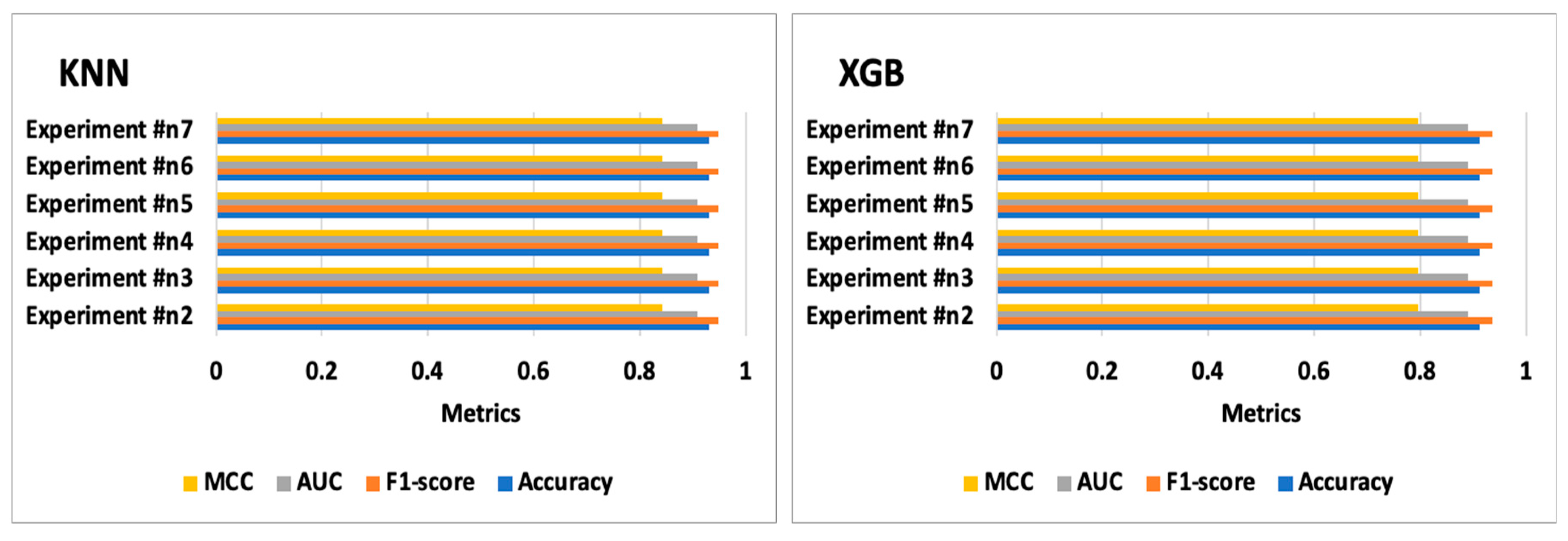
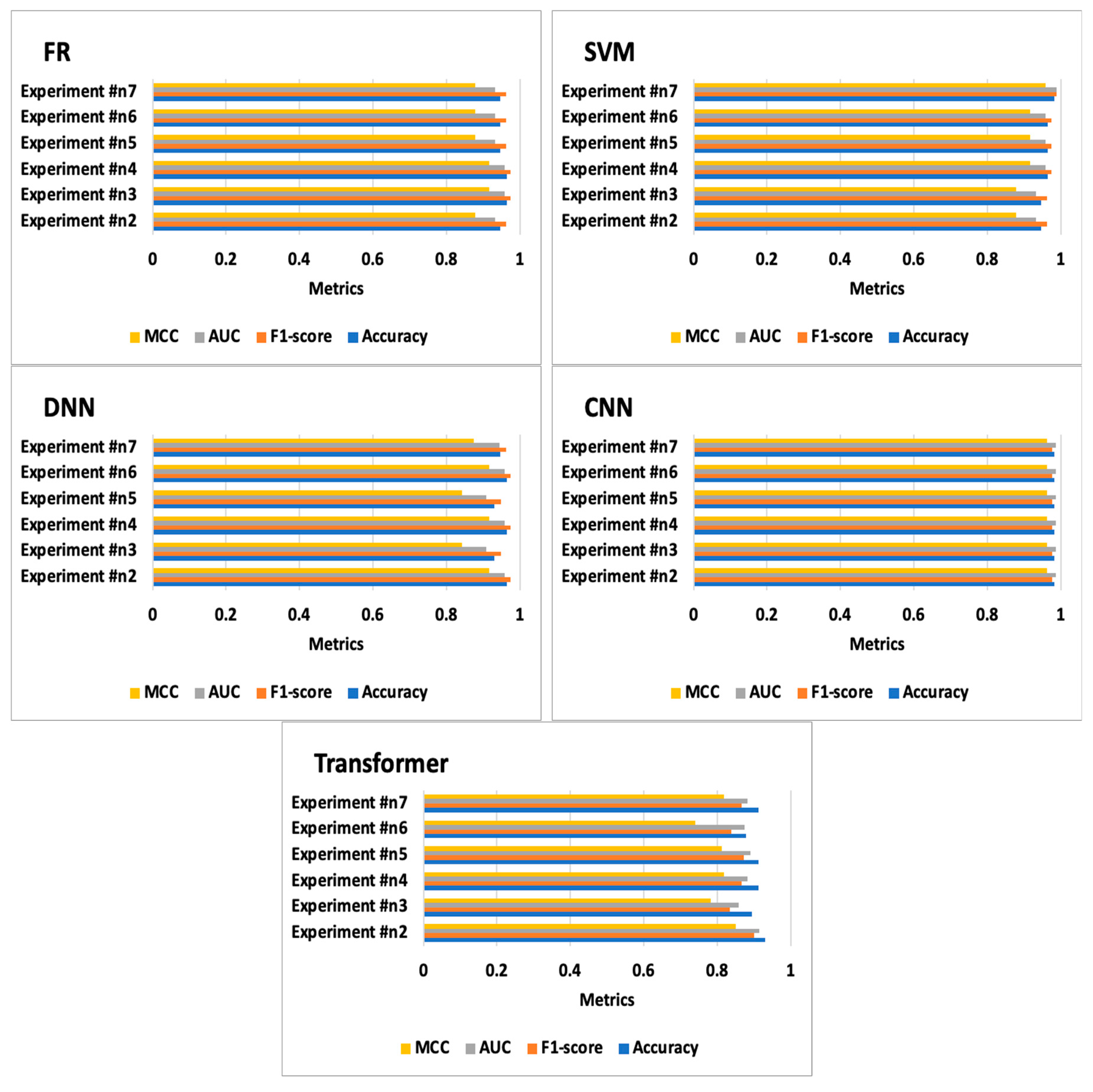
| Experiments | Classifiers | Accuracy | F1-Score | AUC | MCC | Confusion Matrices | Training Time (s) | Test Time (s) |
|---|---|---|---|---|---|---|---|---|
| Experiment #n2 | DNN | 0.965 | 0.975 | 0.958 | 0.916 | [[39 1][1 16]] | 5.528 | 0.093 |
| XGB | 0.912 | 0.937 | 0.891 | 0.795 | [[37 3][2 15]] | 0.030 | 0.004 | |
| RF | 0.947 | 0.962 | 0.932 | 0.877 | [[38 2][1 16]] | 0.133 | 0.004 | |
| SVM | 0.947 | 0.962 | 0.932 | 0.877 | [[38 2][1 16]] | 1.427 | 0.001 | |
| KNN | 0.930 | 0.949 | 0.908 | 0.841 | [[37 3][1 16]] | 0.001 | 0.003 | |
| CNN | 0.982 | 0.977 | 0.986 | 0.963 | [[35 1][0 21]] | 2.061 | 0.116 | |
| Transformer | 0.930 | 0.900 | 0.915 | 0.849 | [[35 1][3 18]] | 1.758 | 0.085 | |
| Experiment #n3 | DNN | 0.930 | 0.949 | 0.908 | 0.841 | [[37 3][1 16]] | 5.648 | 0.093 |
| XGB | 0.912 | 0.937 | 0.891 | 0.795 | [[37 3][2 15]] | 0.029 | 0.003 | |
| RF | 0.965 | 0.975 | 0.958 | 0.916 | [[39 1][1 16]] | 0.133 | 0.004 | |
| SVM | 0.947 | 0.962 | 0.932 | 0.877 | [[38 2][1 16]] | 0.779 | 0.001 | |
| KNN | 0.930 | 0.949 | 0.908 | 0.841 | [[37 3][1 16]] | 0.001 | 0.003 | |
| CNN | 0.982 | 0.977 | 0.986 | 0.963 | [[35 1][0 21]] | 1.992 | 0.129 | |
| Transformer | 0.895 | 0.833 | 0.857 | 0.782 | [[36 0][6 15]] | 1.797 | 0.085 | |
| Experiment #n4 | DNN | 0.965 | 0.975 | 0.958 | 0.916 | [[39 1][1 16]] | 5.449 | 0.099 |
| XGB | 0.912 | 0.937 | 0.891 | 0.795 | [[37 3][2 15]] | 0.029 | 0.003 | |
| RF | 0.965 | 0.975 | 0.958 | 0.916 | [[39 1][1 16]] | 0.132 | 0.004 | |
| KNN | 0.930 | 0.949 | 0.908 | 0.841 | [[37 3][1 16]] | 0.550 | 0.001 | |
| SVM | 0.965 | 0.975 | 0.958 | 0.916 | [[39 1][1 16]] | 0.001 | 0.003 | |
| CNN | 0.982 | 0.977 | 0.986 | 0.963 | [[35 1][0 21]] | 2.020 | 0.112 | |
| Transformer | 0.912 | 0.865 | 0.881 | 0.818 | [[36 0][5 16]] | 1.807 | 0.085 | |
| Experiment #n5 | DNN | 0.930 | 0.949 | 0.908 | 0.841 | [[37 3][1 16]] | 5.425 | 0.093 |
| XGB | 0.912 | 0.937 | 0.891 | 0.795 | [[37 3][2 15]] | 0.030 | 0.003 | |
| RF | 0.947 | 0.962 | 0.932 | 0.877 | [[38 2][1 16]] | 0.131 | 0.004 | |
| KNN | 0.930 | 0.949 | 0.908 | 0.841 | [[37 3][1 16]] | 0.822 | 0.001 | |
| SVM | 0.965 | 0.975 | 0.958 | 0.916 | [[39 1][1 16]] | 0.001 | 0.003 | |
| CNN | 0.982 | 0.977 | 0.986 | 0.963 | [[35 1][0 21]] | 1.996 | 0.114 | |
| Transformer | 0.912 | 0.872 | 0.891 | 0.811 | [[35 1][4 17]] | 1.766 | 0.084 | |
| Experiment #n6 | DNN | 0.965 | 0.975 | 0.958 | 0.916 | [[39 1][1 16]] | 5.379 | 0.095 |
| XGB | 0.912 | 0.937 | 0.891 | 0.795 | [[37 3][2 15]] | 0.029 | 0.003 | |
| RF | 0.947 | 0.962 | 0.932 | 0.877 | [[38 2][1 16]] | 0.133 | 0.004 | |
| KNN | 0.930 | 0.949 | 0.908 | 0.841 | [[37 3][1 16]] | 0.560 | 0.001 | |
| SVM | 0.965 | 0.975 | 0.958 | 0.916 | [[39 1][1 16]] | 0.001 | 0.003 | |
| CNN | 0.982 | 0.977 | 0.986 | 0.963 | [[35 1][0 21]] | 1.996 | 0.113 | |
| Transformer | 0.877 | 0.837 | 0.873 | 0.739 | [[32 4][3 18]] | 1.809 | 0.083 | |
| Experiment #n7 | DNN | 0.947 | 0.963 | 0.944 | 0.873 | [[39 1][2 15]] | 5.403 | 0.095 |
| XGB | 0.912 | 0.937 | 0.891 | 0.795 | [[37 3][2 15]] | 0.036 | 0.004 | |
| RF | 0.947 | 0.962 | 0.932 | 0.877 | [[38 2][1 16]] | 0.132 | 0.004 | |
| KNN | 0.930 | 0.949 | 0.908 | 0.841 | [[37 3][1 16]] | 1.097 | 0.001 | |
| SVM | 0.982 | 0.988 | 0.988 | 0.958 | [[40 0][1 16]] | 0.001 | 0.003 | |
| CNN | 0.982 | 0.977 | 0.986 | 0.963 | [[35 1][0 21]] | 2.020 | 0.122 | |
| Transformer | 0.912 | 0.865 | 0.881 | 0.818 | [[36 0][5 16]] | 1.793 | 0.084 |
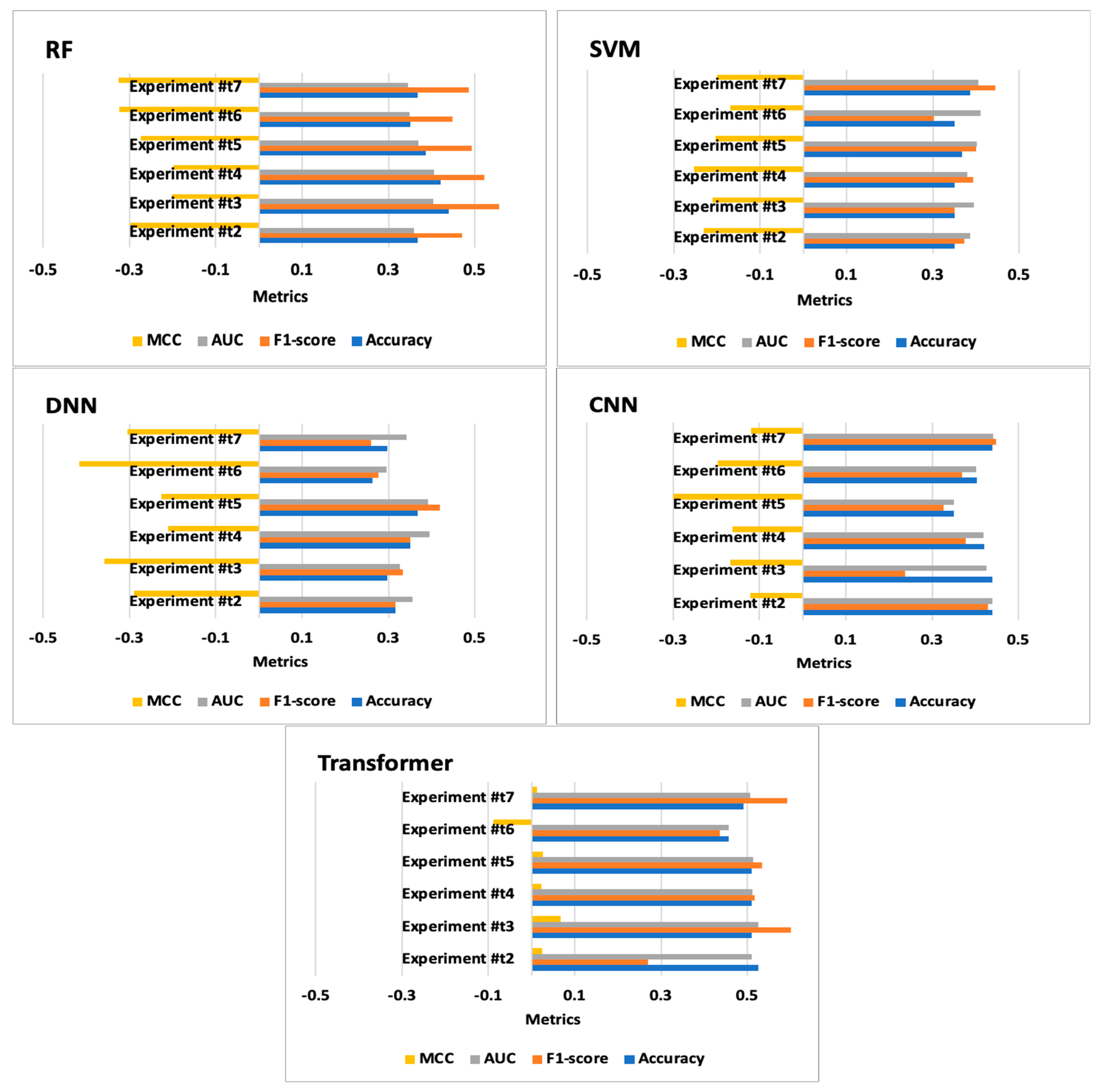
| Experiments | Classifiers | Accuracy | F1-Score | AUC | MCC | Confusion Matrices | Training Time (s) | Test Time (s) |
|---|---|---|---|---|---|---|---|---|
| Experiment #t2 | DNN | 0.316 | 0.316 | 0.355 | −0.289 | [[9 29][10 9]] | 5.445 | 0.097 |
| XGB | 0.421 | 0.522 | 0.406 | −0.199 | [[18 20][13 6]] | 0.044 | 0.003 | |
| RF | 0.368 | 0.471 | 0.359 | −0.298 | [[16 22][14 5]] | 0.211 | 0.004 | |
| SVM | 0.351 | 0.373 | 0.387 | −0.231 | [[11 27][10 9]] | 4.397 | 0.001 | |
| KNN | 0.564 | 0.613 | 0.572 | 0.152 | [[19 19][7 12]] | 0.001 | 0.003 | |
| CNN | 0.439 | 0.429 | 0.439 | −0.122 | [[13 17][15 12]] | 2.026 | 0.114 | |
| Transformer | 0.526 | 0.270 | 0.509 | 0.024 | [[25 5][22 5]] | 1.826 | 0.085 | |
| Experiment #t3 | DNN | 0.298 | 0.333 | 0.327 | −0.357 | [[10 28][12 7]] | 5.661 | 0.094 |
| XGB | 0.421 | 0.522 | 0.406 | −0.199 | [[18 20][13 6]] | 0.045 | 0.003 | |
| RF | 0.439 | 0.556 | 0.403 | −0.202 | [[20 18][14 5]] | 0.214 | 0.004 | |
| SVM | 0.351 | 0.351 | 0.395 | −0.211 | [[10 28][9 10]] | 5.694 | 0.001 | |
| KNN | 0.564 | 0.613 | 0.572 | 0.152 | [[19 19][7 12]] | 0.001 | 0.003 | |
| CNN | 0.439 | 0.238 | 0.426 | −0.168 | [[20 10][22 5]] | 1.981 | 0.113 | |
| Transformer | 0.509 | 0.622 | 0.526 | 0.068 | [[6 24][4 23]] | 1.760 | 0.084 | |
| Experiment #t4 | DNN | 0.351 | 0.351 | 0.395 | −0.211 | [[10 28][11 8]] | 5.484 | 0.097 |
| XGB | 0.421 | 0.522 | 0.406 | −0.199 | [[18 20][13 6]] | 0.047 | 0.005 | |
| RF | 0.421 | 0.522 | 0.406 | −0.199 | [[18 20][13 6]] | 0.213 | 0.004 | |
| KNN | 0.564 | 0.613 | 0.572 | 0.152 | [[19 19][7 12]] | 3.752 | 0.001 | |
| SVM | 0.351 | 0.393 | 0.379 | −0.253 | [[12 26][11 8]] | 0.001 | 0.003 | |
| CNN | 0.421 | 0.377 | 0.419 | −0.163 | [[14 16][17 10]] | 1.985 | 0.109 | |
| Transformer | 0.509 | 0.517 | 0.511 | 0.022 | [[14 16][12 15]] | 1.777 | 0.085 | |
| Experiment #t5 | DNN | 0.368 | 0.419 | 0.392 | −0.226 | [[13 25][11 8]] | 5.454 | 0.096 |
| XGB | 0.421 | 0.522 | 0.406 | −0.199 | [[18 20][13 6]] | 0.044 | 0.003 | |
| RF | 0.386 | 0.493 | 0.370 | −0.274 | [[17 21][14 5]] | 0.217 | 0.004 | |
| KNN | 0.564 | 0.613 | 0.572 | 0.152 | [[19 19][7 12]] | 7.574 | 0.001 | |
| SVM | 0.368 | 0.400 | 0.401 | −0.204 | [[12 26][10 9]] | 0.001 | 0.003 | |
| CNN | 0.351 | 0.327 | 0.350 | −0.300 | [[11 19][18 9]] | 2.020 | 0.108 | |
| Transformer | 0.509 | 0.533 | 0.513 | 0.026 | [[13 17][11 16]] | 1.793 | 0.087 | |
| Experiment #t6 | DNN | 0.263 | 0.276 | 0.295 | −0.416 | [[8 30][12 7]] | 5.410 | 0.094 |
| XGB | 0.421 | 0.522 | 0.406 | −0.199 | [[18 20][13 6]] | 0.045 | 0.003 | |
| RF | 0.351 | 0.448 | 0.348 | −0.323 | [[15 23][14 5]] | 0.215 | 0.004 | |
| KNN | 0.564 | 0.613 | 0.572 | 0.152 | [[19 19][7 12]] | 10.461 | 0.001 | |
| SVM | 0.351 | 0.302 | 0.410 | −0.169 | [[8 30][7 12]] | 0.001 | 0.003 | |
| CNN | 0.404 | 0.370 | 0.402 | −0.196 | [[13 17][17 10]] | 2.042 | 0.113 | |
| Transformer | 0.456 | 0.436 | 0.456 | −0.089 | [[14 16][15 12]] | 1.803 | 0.085 | |
| Experiment #t7 | DNN | 0.298 | 0.259 | 0.341 | −0.304 | [[7 31][9 10]] | 5.413 | 0.094 |
| XGB | 0.421 | 0.522 | 0.406 | −0.199 | [[18 20][13 6]] | 0.047 | 0.004 | |
| RF | 0.368 | 0.486 | 0.346 | −0.325 | [[17 21][15 4]] | 0.216 | 0.004 | |
| KNN | 0.564 | 0.613 | 0.572 | 0.152 | [[19 19][7 12]] | 5.225 | 0.001 | |
| SVM | 0.386 | 0.444 | 0.405 | −0.200 | [[14 24][11 8]] | 0.001 | 0.003 | |
| CNN | 0.439 | 0.448 | 0.441 | −0.119 | [[12 18][14 13]] | 2.009 | 0.108 | |
| Transformer | 0.491 | 0.592 | 0.506 | 0.013 | [[7 23][6 21]] | 1.767 | 0.097 |
Disclaimer/Publisher’s Note: The statements, opinions and data contained in all publications are solely those of the individual author(s) and contributor(s) and not of MDPI and/or the editor(s). MDPI and/or the editor(s) disclaim responsibility for any injury to people or property resulting from any ideas, methods, instructions or products referred to in the content. |
© 2025 by the authors. Licensee MDPI, Basel, Switzerland. This article is an open access article distributed under the terms and conditions of the Creative Commons Attribution (CC BY) license (https://creativecommons.org/licenses/by/4.0/).
Share and Cite
Moldovanu, S.; Munteanu, D.; Sîrbu, C. Impact on Classification Process Generated by Corrupted Features. Big Data Cogn. Comput. 2025, 9, 45. https://doi.org/10.3390/bdcc9020045
Moldovanu S, Munteanu D, Sîrbu C. Impact on Classification Process Generated by Corrupted Features. Big Data and Cognitive Computing. 2025; 9(2):45. https://doi.org/10.3390/bdcc9020045
Chicago/Turabian StyleMoldovanu, Simona, Dan Munteanu, and Carmen Sîrbu. 2025. "Impact on Classification Process Generated by Corrupted Features" Big Data and Cognitive Computing 9, no. 2: 45. https://doi.org/10.3390/bdcc9020045
APA StyleMoldovanu, S., Munteanu, D., & Sîrbu, C. (2025). Impact on Classification Process Generated by Corrupted Features. Big Data and Cognitive Computing, 9(2), 45. https://doi.org/10.3390/bdcc9020045