A Recursive Attribute Reduction Algorithm and Its Application in Predicting the Hot Metal Silicon Content in Blast Furnaces

Abstract

For many complex industrial applications, traditional attribute reduction algorithms are often inefficient in obtaining optimal reducts that align with mechanistic analyses and practical production requirements. To solve this problem, we propose a recursive attribute reduction algorithm that calculates the optimal reduct. First, we present the notion of priority sequence to describe the background meaning of attributes and evaluate the optimal reduct. Next, we define a necessary element set to identify the “individually necessary” characteristics of the attributes. On this basis, a recursive algorithm is proposed to calculate the optimal reduct. Its boundary logic is guided by the conflict between the necessary element set and the core attribute set. The experiments demonstrate the proposed algorithm’s uniqueness and its ability to enhance the prediction accuracy of the hot metal silicon content in blast furnaces.

1. Introduction

Introduced by Pawlak in 1982, rough set theory serves as a mathematical tool for dealing with vague, imprecise, and uncertain knowledge, garnering increasing attention in computer sciences, artificial intelligence, medical applications, etc. [1,2]. Attribute reduction, a core aspect of rough set theory, simplifies datasets by eliminating irrelevant attributes, which is commonly known as feature selection in machine learning [3,4,5]. Over the last decades, researchers have developed many heuristic reduction algorithms based on the positive region [6,7,8,9], the discernibility matrix [10,11], and information entropy [12,13,14]. While these algorithms have achieved efficiency in running time and storage, they are not always effective in obtaining the optimal reduct when used in complex industrial applications, especially in blast furnace smelting, because they overlook the underlying industrial mechanisms embedded in the data. Without these mechanistic insights, current techniques may discard essential attributes or retain unnecessary ones, leading to suboptimal reductions with limited practical utility.

Blast furnace smelting is the most energy-consuming process in iron and steel production [15,16]. Its internal state is difficult to measure directly because of the influence of high temperature and high pressure. Fortunately, extensive research has demonstrated that the silicon content in hot metal exhibits a close relationship with its thermal state [17,18,19]. Thus, the accurate prediction of the hot metal silicon content is key to the optimal control of blast furnaces.

As a classical complex industrial process, the accuracy of a silicon content prediction depends not only on excellent nonlinear models but also on high-quality datasets. However, due to the strong parameter coupling and nonlinear characteristics of blast furnace systems, original datasets often contain a large number of redundant attributes. It is therefore necessary to calculate a reduction set to improve the training speed and prediction accuracy.

According to rough set theory, there may be multiple complete reduction sets in a dataset. Traditional algorithms, however, only compute one of them at random. From the perspective of blast furnace mechanisms, each attribute has its specific physical meaning and reflects different aspects of the furnace. This means that different reduction sets represent different information, and there should be an optimal reduction set corresponding to both the mechanistic analysis and practical production. Therefore, determining the optimal reduction set represents a meaningful research task.

In addition, how the optimal reduction set of a blast furnace is evaluated is also necessary to consider. In previous studies, many researchers have used the test costs of attributes to evaluate a reduction set, believing that the minimum cost is optimal [20,21,22,23]. However, related smelting mechanism analyses and practical production experience have shown that it is hard to set the exact numerical cost for all attributes. Instead, researchers have achieved better results when analyzing which attributes are more important.

Motivated by the above observations, we suggest an importance sequence, called the attribute priority sequence, in this paper to describe the background meaning of the attributes and prior knowledge related to the blast furnace. On this basis, a priority-optimal reduct is defined, and a novel attribute reduction algorithm using recursion technology is proposed to calculate it. Some experimental results on UCI datasets show differences between the proposed algorithm, classical method, and state-of-the-art method. We also applied this algorithm on a real dataset obtained from a blast furnace, and we trained a machine learning model to show the proposed algorithm’s performance. The major contributions of this paper are as follows:

(1)

We propose a novel heuristic reduction construction.

Existing heuristic reduction algorithms commonly adopt the following three kinds of construction: addition–deletion constructions (Algorithm 1), deletion constructions, and addition constructions. In this paper, we propose a novel recursion construction that is effective in obtaining special reducts, such as the optimal reduct, minimal reduct, and minimal cost reduct.

Algorithm 1. Traditional heuristic attribute reduction algorithm.

Input: Information table $S$ and priority sequence $\left\{c_1,c_2,\dots ,c_n\right\}.$ Output: Reduct $R$. Step 1: Construct the discernibility matrix, $M$; calculate the core attribute set, $CORE\left(M\right)$; and the delete elements discerned by $CORE\left(M\right)$. Step 2: Delete the attributes belonging to $CORE\left(M\right)$ from the priority sequence; then, the new priority sequence is $\{c_{i1},c_{i2},\dots ,c_{im}$}. Step 3: Addition: $\hspace{1em}R\prime =\varnothing$, k = 1. While $R\prime$ is not a super reduct of $M$, do $\hspace{1em}\hspace{1em}\hspace{1em}\hspace{1em}\hspace{1em}\hspace{1em}\hspace{1em}\hspace{1em}\hspace{1em}\hspace{1em}\hspace{1em}\hspace{1em}\hspace{1em}R\prime =R\prime \cup c_{ik},k=k+1$ End Step 4: Deletion: While $k>0$, do If $R\prime -\left\{c_{ik}\right\}$ is a super reduct then $\hspace{1em}\hspace{1em}\hspace{1em}\hspace{1em}\hspace{1em}\hspace{1em}\hspace{1em}\hspace{1em}\hspace{1em}\hspace{1em}\hspace{1em}\hspace{1em}\hspace{1em}\hspace{1em}\hspace{1em}R\prime =R\prime -\left\{c_{ik}\right\}$ End      k = k − 1 End Step 5: Output $R=R\prime \cup CORE\left(M\right)$

(2)

We define a new optimal reduct.

Traditional rough set theories often treat a minimal reduct as optimal because they ignore related prior knowledge. Many researchers have applied the notion of “cost” to describe prior knowledge and treated a minimal cost reduct as optimal. As mentioned above, “cost” is not always effective in complex situations because it is hard to set the exact costs for all attributes. Therefore, we propose the notion of an attribute priority sequence and define a priority-optimal reduct to represent an optimal reduct. The new definition of the optimal reduct is simple and suitable for complex applications.

(3)

We provide a recursive reduction algorithm and illustrate its validity based on UCI datasets and a real application on silicon content prediction.

The proposed algorithm is the first recursion-based reduction algorithm, and the detailed reasoning, as well as the experimental results, show its validity. Furthermore, the proposed algorithm heuristically identifies a priority-optimal reduct.

The rest of this study is organized as follows. Section 2 presents some basic knowledge on Pawlak rough set. Section 3 presents the definition of the priority-optimal reduct and proposes an attribute reduction algorithm using recursion technology to obtain the priority-optimal reduct. Section 4 discusses the experiments and results of hot metal silicon content prediction in blast furnaces.

2. Preliminary Knowledge on Pawlak Rough Set

In rough set theory, data are presented in an information table S [7].

$$S=〈U,At,\left\{V_a|a\in At\right\},\left\{I_a|a\in At\right\}〉$$

where U is the universe, At is a finite non-empty set of attributes, V_a is a non-empty set of values of attribute a, and $I_a:U\to V_a$ is an information function that maps an object in $U$ to exactly one value in V_a. As a special type, an information table S is also referred to as a decision table if $At=C\cup D$, where $C=\left\{c_1,c_2,\dots ,c_n\right\}$ is the condition attribute set and $D=\left\{d\right\}$ is the decision attribute set. A decision table is inconsistent if it contains two objects with the same condition values but different decision values.

Definition 1.

Given a subset of attributes  $B\subseteq C,$ an indiscernibility relationship  $IND\left(B\right)$ is defined as follows.

$$IND\left(B\right)=\left\{\left(x,x\prime \right)\in U^2 |\forall a\in B,I_a\left(x\right)=I_a\left(x\prime \right)\right\}$$

(1)

The equivalence class (or granule) of object $x$ with respect to $C$ is ${\left[x\right]}_C=\{y\in U |\left(x,y\right)\in IND\left(C\right)\}$. The union of all the granules with respect to $C$ is referred to as a partition of the universe, described as $U/C=\{{\left[x\right]}_C |x\in U\}$. Granule ${\left[x\right]}_C$ is exact if it has only one decision value; otherwise, it is rough. The union of all the exact granules with respect to $C$ is referred to as the positive region, described as $PO{S}_C \left(D\right)=\left\{{\left[x\right]}_C\right|\left|I_d\left({\left[x\right]}_C\right)\right|=1\}$. Based on the indiscernibility relationship and the positive region, a discernibility matrix is defined as follows.

Definition 2.

Given an information table  $S,$ a discernibility matrix  $M$ based on the positive region is defined as

$$m\left(i,j\right)=\left\{\begin{array}{c}\left\{a\in C|I_a\left(x_i\right)\ne I_a\left(x_j\right)\right\},I_d\left(x_i\right)\ne I_d\left(x_j\right)\wedge \left(x_i\in PO{S}_C \left(D\right)\vee x_j\in PO{S}_C \left(D\right)\right)\\ \\ \varnothing , \mathrm{else} \end{array}\right.$$

(2)

Definition 3.

Given an information table  $S,$ an attribute set  $R\subseteq At$ is called a reduct if it satisfies the following two conditions [7]:

(1) 

$IND\left(R\right)=IND\left(At\right)$;

(2) 

$\forall a\in R,IND\left(R-\left\{a\right\}\right)\ne IND\left(At\right)$.

If a discernibility matrix  $M=\left\{m\left(i,j\right)\right\}$ is constructed, then the two conditions mentioned above can be described as follows:

(1) 

$\forall m\left(i,j\right)\ne \varnothing \Rightarrow R\cap m\left(i,j\right)\ne \varnothing$;

(2) 

$\forall a\in R,\exists m\left(i,j\right)\ne \varnothing \wedge m\left(i,j\right)\cap \left(R-\left\{a\right\}\right)=\varnothing$.

A reduct is a subset of attributes that is “jointly sufficient and individually necessary” to represent the knowledge equivalent to the attribute set $C$. In general, an information table may have multiple reducts. The set of these reducts is denoted as $RED\left(S\right)$, and the intersection of all reducts is the core set, $Core\left(S\right)=\cap RED\left(S\right)$ or $Core\left(M\right)={{\displaystyle \cup }}_{\left|m\left(i,j\right)\right|=1}m\left(i,\mathrm{j}\right)$. If an attribute subset $R\prime$ only satisfies the first condition, then it is referred to as a super reduct, i.e., $\exists R\in RED\left(S\right), R\subseteq R\prime$.

3. Recursive Attribute Reduction Algorithm Based on Priority Sequence

In this section, a priority-optimal reduct is defined first. Subsequently, a heuristic approach is discussed, and an attribute reduction algorithm based on a priority sequence is proposed using recursion.

3.1. Priority Sequence and Priority-Optimal Reduct

In this paper, prior knowledge of a blast furnace is treated as a priority sequence of attributes. For a priority sequence $\left\{c_1,c_2,\dots ,c_n\right\}$, attribute $c_1$ has the highest priority, and $c_n$ has the lowest priority. In practical applications, we can determine this sequence based on empirical knowledge or mechanistic analysis results. In other words, when assigning numbers to these attributes, those deemed more important are placed at the front. The priority-optimal reduct is thus defined as follows.

Definition 4.

Given a discernibility matrix  $M$ and a priority sequence  $\left\{c_1,c_2,\dots ,c_n\right\}$, a reduct  $R\in RED\left(M\right)$ is called the priority-optimal  reduct ($POR$) if  $\forall R^{\prime }\in RED\left(M\right)-R,\exists c\in R-\left(R\cap R^{\prime }\right), so that p\left(c\right)>p\left(c\prime \right)$, where $p\left(c\right)$ is the priority of attribute $c$, and $c\prime \in R\prime -\left(R\cap R\prime \right)$.

Based on Definition 4, it is straightforward to conclude that POR is unique for a given priority sequence. In other words, each priority sequence can accurately map a corresponding POR. Hence, if the priority sequence represents prior knowledge, then POR is the optimal solution.

However, even though the priority sequence is taken into account, it is still difficult for the traditional attribute reduction algorithm (shown in Algorithm 1) to obtain the POR. A typical example is shown in Example 1.

Example 1.

Suppose a discernibility matrix  $M$ has four non-empty elements: $\left\{a,b\right\}, \left\{a,c\right\}, \left\{b,d\right\}$, and  $\left\{c,d\right\}$.

For a priority sequence $\left\{a,b,c,d\right\}$, it obtains  $R\prime =\left\{a,b,c\right\}$ after step 3, and the attribute “a” is removed in step 4, yielding the  reduct  $\left\{b,c\right\}$. However, the matched  $POR$ is  $\left\{a,d\right\}$ because attribute “a” has a higher priority.

Example 1 illustrates that the traditional attribute reduction algorithm is not suitable for calculating POR because high-priority attributes may be removed during the reduction process. In other words, a combination of lower-priority attributes replaces an attribute with a higher priority. Therefore, to obtain POR, new approaches are necessary to avoid this outcome.

3.2. Calculation Method on POR

For a heuristic reduction algorithm, each condition attribute is evaluated in turn according to the given priority sequence $\{c_1,c_2,\dots ,c_n\}$. The key challenge is to determine whether the evaluated condition attribute belongs to POR. Next, we analyze how to identify the first attribute of POR and the remaining attributes, respectively.

3.2.1. Calculation of the First Attribute of POR

Theorem 1.

For a priority sequence $\left\{c_1,c_2,\dots ,c_n\right\}$, if  $\exists R\in RED\left(M\right)$ so that $c_1\in R$, then $c_1\in POR$.

Proof. 

For $\forall R\prime \in RED\left(M\right)$, if $\left\{c_1\right\}\cap R\prime =\varnothing$, it has $p\left(c_1\right)$ > max(p(c′)), where $c\prime \in R\prime -\left(R\cap R\prime \right)$. According to Definition 4, R’ is not the POR. In other words, POR includes attribute $c_1$. □

According to Theorem 1, the first attribute of POR can be found using the following approach.

Approach 1.

Attribute  $c_i$ is the first attribute of  $POR$ if it satisfies the following two conditions:

$\exists R\in RED\left(M\right)$, $c_i\in R$;

$\forall c\in C, if p\left(c\right)>p\left(c_i\right)$, then $\left\{c\right\}\cap \left(\cup RED\left(M\right)\right)=\varnothing$.

However, calculating all the reducts $RED\left(M\right)$ is impractical in a heuristic algorithm. Thus, the notions of free matrix and absolute redundant attribute set are proposed in this paper to identify the first attribute of POR.

Definition 5.

The absolute redundant attribute set of a decision table  $S$ is defined as

$$ARAS\left(S\right)=\left\{\mathrm{c}\in \mathrm{C}|\forall \mathrm{R}\in \mathrm{RED}\left(\mathrm{S}\right),\mathrm{c}\notin \mathrm{R}\right\}$$

(3)

$ARAS\left(S\right)$is also referred to as  $ARAS\left(M\right)$ if a discernibility matrix  $M$ is considered. Based on Definition 5, one can derive the following properties:

(1) 

$Core\left(M\right)\cap ARAS\left(M\right)=\varnothing$;

(2) 

$\forall c\in C$, if $c\notin ARAS\left(M\right)$, then $\exists R\in RED\left(M\right)$, $c\in R$;

(3) 

$ARAS\left(M\right)\cap POR=\varnothing$.

Theorem 2.

Given a discernibility matrix  $M$ and an attribute priority sequence $\{c_1,c_2,\dots ,c_n\}$, if $ARAS\left(M\right)=\varnothing$, then  $c_1$ is the first attribute of $POR$.

Proof. 

Based on Definitions 4 and 5, since $ARAS\left(M\right)=\varnothing$, $\exists R\in RED\left(M\right),$$c_1\in R$. Considering that $c_1$ has the highest priority, $c_1$ must belong to POR, and it is its first attribute. □

If $ARAS\left(M\right)\ne \varnothing$, one can remove $ARAS\left(M\right)$ from the discernibility matrix to calculate the first attribute of POR. The resulting discernibility matrix is referred to as a free matrix, defined as follows.

Definition 6.

Discernibility matrix  $M$is a free matrix if, for any non-empty elements $m\left(x,y\right),m\left(x\prime ,y\prime \right)\in M$, it holds that $m\left(x,y\right)\not\subset m\left(x\prime ,y\prime \right)$.

The free matrix M does not contain any absolute redundant attribute, and the relevant analysis is presented below.

Theorem 3.

Given discernibility matrix $M$, if  $\forall m\left(x,y\right),m\left(x\prime ,y\prime \right)\in M$, $m\left(x,y\right)\not\subset m\left(x\prime ,y\prime \right)$, then  $ARAS\left(M\right)=\varnothing$.

Proof. 

For any attribute $c\in C$, if $c$ is a core attribute, then $c\notin ARAS\left(M\right)$. If attribute $c$ is not a core attribute, let $M=M_c+M_c\prime$, where $M_c=\{m\left(x,y\right)\in M|c\in m\left(x,y\right)\}$, $M_c\prime =\{m\left(x,y\right)\in M|c\notin m\left(x,y\right)\}$. Select an element $m\left(p,q\right)\in M_c$ and define $A=m\left(p,q\right)-\left\{c\right\}$. One can construct a new discernibility matrix $M\prime =\{m\prime \left(x,y\right)|m\prime \left(x,y\right)=m\left(x,y\right)-A\}$. Matrix $M^{\prime }$ clearly has the following features: (1) attribute $\mathrm{c}$ is a core attribute of $M^{\prime }$ and (2) under the existing condition ($m\left(x,y\right)\not\subset m\left(x\prime ,y\prime \right)$), $\left|m\left(x,y\right)\cup m\left(x\prime ,y\prime \right)-\left(m\left(x,y\right)\cap m\left(x\prime ,y\prime \right)\right)\right|\ge 2$. Thus, for any non-empty element $m\left(x,y\right)\in M$, $m\prime \left(x,y\right)\ne \varnothing$. Hence, based on Definition 3, $C-A$ is a super reduct of $M$ and $\forall R^{\prime }\in RED\left(M\prime \right), R\prime \in RED\left(M\right)$. Since $c\in CORE\left(M\prime \right)$, there exists a reduct $R\prime$ that includes $c$. Therefore, attribute $c$ is not a redundant attribute in $R\prime$, and $ARAS\left(M\right)=\varnothing$. □

Based on Theorems 2 and 3, we obtain an important approach.

Approach 2.

The highest priority attribute of a free matrix is the first attribute of POR.

The free matrix is constructed by Algorithm 2.

Algorithm 2. Construct the free matrix.

Input: Discernibility matrix $M$. Output: The related free matrix. Step 1: Sort all the non-empty elements $m\left(x,y\right)$ by $\left|m\left(x,y\right)\right|$; let $num$ be the number of non-empty elements. Step 2: Set $i=1$  While $i\le num-1$, do $j=i+1$; While $j\le num$, do If $m_i\left(x,y\right)\subset m_j\left(x,y\right)$ then          delete $m_j\left(x,y\right)$ from $M\prime$, $num=num-1$        Else           $j=j+1$.        End     End                $i=i+1$  End Step 3: Output the free matrix.

3.2.2. Calculation on Other Attributes of POR

Besides the first attribute, the other attributes of POR are checked according to Theorem 4.

Theorem 4.

For attribute $c_{k+1}$, if  $\exists R\in RED\left(M\right)$, $B_k\cup \left\{c_{k+1}\right\}\subseteq R$, then $c_{k+1}\in POR$, where  $B_k=POR\cap A_k$ and  $A_k=\left\{c_1,c_2,\dots ,c_k\right\}$.

Proof. 

Let $P=POR-B_k$. According to the definition of $B_k$, the attribute set $P$ is a subset of $C-A_k$. Since there exists a reduct $R$ that includes $B_k$ and attribute $c_{k+1}$, $B_k$ cannot discern all elements of matrix $M$, i.e., $P\ne \varnothing$. Suppose $c_{k+1}\notin POR$. In that case, the reduct $R$ is not POR. However, $\forall c\in P$, $c_{k+1}\in R-B_k$ satisfies $p\left(c_{k+1}\right)>p\left(c\right)$. This conflicts with Definition 4. Hence, the above assumption is invalid, implying $c_{k+1}\in POR$. □

According to Theorem 4, the conclusion is that the key step is to verify whether there exists a reduct that contains both $c_{k+1}$ and the attribute set $B_k=POR\cap \left\{c_1,c_2,\dots ,c_k\right\}$.

Considering that a reduct should be “jointly effective and individually necessary,” we introduce the notion of the necessary element set to represent “individually necessary.”

Definition 7.

Given a discernibility matrix $M=\left\{m\left(x,y\right)\right\}$, the necessary element set ($NES$) of attribute c with respect to attribute set  $B$ is  $NE{S}_B\left(c\right)=\left\{m\left(x,y\right)\right|m\left(x,y\right)\cap B=\left\{c\right\}\}$.

The notion of $\mathrm{NES}$ is similar to that of a core set, since both are related to “necessary”. The core set represents the attributes that are necessary for all reducts. Meanwhile, $NE{S}_B\left(c\right)$ indicates whether attribute $\mathrm{c}$ is necessary to attribute set $B$. It has the following:

(1)

$CORE\left(M\right)=\{c\in C|NE{S}_C\left(c\right)\ne \varnothing \}$;

(2)

If $\left\{c\right\}\subseteq A_1\subseteq A_2,$ then $NE{S}_{A_2}\left(c\right)\subseteq NE{S}_{A_1}\left(c\right)$.

If $NE{S}_B\left(c\right)\ne \varnothing$, then the attribute set $B-\left\{c\right\}$ is not a reduct because it cannot discern the non-empty elements in $NE{S}_B\left(c\right)$. Conversely, if $NE{S}_B\left(c\right)=\varnothing$, then $\forall m\left(x,y\right)\cap \left\{c\right\}\ne \varnothing$, $m\left(x,y\right)\cap \left(B-\left\{c\right\}\right)\ne \varnothing$. This means that all elements discerned by attribute $c$ are also discerned by $B-\left\{c\right\}$. Thus, attribute set $B$ is not a reduct.

Based on the above analysis, we redefine the reduct using $\mathrm{NES}$.

Definition 8.

An attribute set R is called a reduct if and only if it satisfies the following conditions:

(1) 

For each non-empty element $m\left(x,y\right)\in M$, $m\left(x,y\right)\cap R\ne \varnothing$;

(2) 

For each attribute $c\in R$, $NE{S}_R\left(c\right)\ne \varnothing$.

Based on Definition 8, we have the following conclusion about $NE{S}_B\left(c\right)$.

Theorem 5.

Given a discernibility matrix  $M=\left\{m\left(x,y\right)\right\}$ and an attribute set $B\subseteq C$, if there exists a  reduct  $R\in RED\left(M\right)$ that includes the attribute set $B$, then $\forall c\in B,NE{S}_B\left(c\right)\ne \varnothing$.

Proof. 

Based on Definition 8, $R$ satisfies $\forall c\in R$, $NE{S}_R\left(c\right)\ne \varnothing$. Because $B\subseteq R$, we have $\forall c\in B,NE{S}_B\left(c\right)\ne \varnothing$ since $NE{S}_R\left(c\right)\subseteq NE{S}_B\left(c\right)$. □

According to Theorem 5, if $\exists c\in B, NE{S}_B\left(c\right)=\varnothing$, then no reduct can include $B$.

Based on the above discussions, we propose a recursive algorithm to determine the other attributes of POR. Recursion is a kind of self-relation and is represented as a function capable of calling itself within a program. Once a recursive function calls itself, it reduces a problem into sub-problems. The recursive call process continues until it reaches an end point where the sub-problem cannot be reduced further. Thus, there are two elements in a recursive method: simple repeated logic and a termination condition. In this paper, an additional border logic is also adopted to ensure that the result is a reduct.

• Simple Repeated Logic

Repeated logic refers to the similarity between a problem and its sub-problems, which constitutes the main part of recursion.

In this method, repeated logic is utilized to verify the existence of a reduct that includes $B_k\cup \left\{c_{k+1}\right\}$, and it can be divided into two parts: (1) calculation $\mathrm{NES}$ and (2) judgment logic. The $\mathrm{NES}$ calculation of $B_k\cup \left\{c_{k+1}\right\}$ is based on Definition 7, and further descriptions are unnecessary. For the judgment logic, there are two cases.

(1)

If $\forall c\in B_k\cup \left\{c_{k+1}\right\},NE{S}_{B_k+\left\{c_{k+1}\right\}}\left(c\right)\ne \varnothing$, then we accept $c_{k+1},$ $B_{k+1}=B_k\cup \left\{c_{k+1}\right\}$, and we call this method with the updated parameter set.

(2)

If $\exists c\in B_k\cup \left\{c_{k+1}\right\},NE{S}_{B_k\cup \left\{c_{k+1}\right\}}\left(c\right)=\varnothing$, then we reject $c_{k+1}, B_{k+1}=B_k$, and we remove $c_{k+1}$ from the discernibility matrix.

A simple example is described as follows.

Example 2.

Given  $M=\left\{\left\{a,b\right\}, \left\{a,c\right\}, \left\{b,d\right\}, \left\{c,d\right\}\right\}$ and the priority sequence  $\left\{a,b,c,d\right\}$,  $M$ is a free matrix.

First, according to Approach 2, attribute $a$ is the first attribute of POR. Next, B₁ = {a} and the other attributes are evaluated in turn.

For attribute $b$, $NE{S}_{B_1\cup \left\{b\right\}}\left(a\right)=\left\{\left\{a,c\right\}\right\}, NE{S}_{B_1\cup \left\{b\right\}}\left(b\right)=\left\{\left\{b,d\right\}\right\}$. Attribute $b$ is accepted, and the attribute set becomes $B_2=\left\{a,b\right\}$.

For attribute $c$, $B_2=\left\{a,b\right\},$ $NE{S}_{B_2\cup \left\{c\right\}}\left(a\right)=\varnothing , NE{S}_{B_2\cup \left\{c\right\}}\left(b\right)=\left\{\left\{b,d\right\}\right\},NE{S}_{B_2+\left\{c\right\}}\left(c\right)=\left\{\left\{c,d\right\}\right\}$. Since $NE{S}_{B_2\cup \left\{c\right\}}\left(a\right)=\varnothing$, attribute c is rejected and the new matrix is $M_1=\left\{\left\{a,b\right\}, \left\{a\right\}, \left\{b,d\right\}, \left\{d\right\}\right\},$ $B_3=B_2=\left\{a,b\right\}$.

• Additional Border Logic

Since the logic above uses only a necessary condition to test attributes in priority sequence order, we will encounter a border during recursion, referred to here as core conflict.

Definition 9.

Given a discernibility matrix  $M$, attribute set$B$, and a core attribute  $c\prime \in CORE\left(M\right)$, the core conflict between  $B$ and  $c\prime$($c\prime \notin B$) is described as follows:  $\exists c\in B, NE{S}_B\left(c\right)\ne \varnothing$,  $NE{S}_{B\cup \left\{c\prime \right\}}\left(c\right)=\varnothing$.

Since $c\prime \in CORE\left(M\right)$, $c\prime$ must belong to all reducts. However, due to this core conflict, no reduct can include both $B$ and $c\prime$. Thus, we present the following approach.

Approach 3.

Given a discernibility matrix  $M$ and an attribute set$B$, if there is a core conflict between  $B$ and a core attribute, then no  reduct can include $B$.

At the start of this method, no core attribute exists in the free matrix $M$ because of step 1 of Algorithm 1. As recursion proceeds, some attributes are removed from $M$, which causes certain attributes to become core attributes in the new discernibility matrix $M_k$. If these core attributes conflict with higher-priority attributes, a core conflict will arise in the recursion.

The occurrence of core conflicts implies that at least one redundant attribute is present. The simplest way to address this is to remove any attributes for which $NE{S}_{B\cup \left\{c^{\prime }\right\}}\left(c\right)=\varnothing$ from the related discernibility matrix. By doing so, we eventually obtain a reduct. However, this reduct may not be POR. A simple example is provided in Example 3.

Example 3.

Given  $M=\{\left\{a,b\right\}$,$\left\{a,e\right\}$,$\left\{b,d\right\}$,$\left\{c,e\right\}$,  $\left\{d,e\right\}\}$ and the priority sequence  $\left\{a,b,c,d,e\right\}$,  $M$ is a free matrix, and attribute  $a$ is the first attribute of POR. Using repeated logic, we obtain  $B_3=\left\{a,b,c\right\}, NE{S}_{B_3}\left(a\right)=\left\{\left\{a,e\right\}\right\}, NE{S}_{B_3}\left(b\right)=\left\{\left\{b,d\right\}\right\},NE{S}_{B_3}\left(c\right)=\left\{\left\{c,e\right\}\right\}$. For the next attribute $d$, we find $NE{S}_{B_3\cup \left\{d\right\}}\left(b\right)=\varnothing$, and  $d$ is not a core attribute. Attribute  $d$ is then removed from $M$, producing  $M_1=\left\{\left\{a,b\right\}, \left\{a,e\right\}, \left\{b\right\}, \left\{c,e\right\}, \left\{e\right\}\right\}$. For the last attribute  $e$,  $NE{S}_{B_3\cup \left\{e\right\}}\left(a\right)=\varnothing , NE{S}_{B_3\cup \left\{e\right\}}\left(b\right)=\left\{\left\{b\right\}\right\}$,  $NE{S}_{B_3\cup \left\{e\right\}}\left(c\right)=\varnothing$. Since  $e$ is a core attribute, it cannot be removed. In this case, the core attribute$e$conflicts with two higher-priority attributes  $a$ and $c$. If the conflict is ignored, the attribute set $\left\{b,e\right\}$would be obtained by removing  $a$and$c$. Clearly,  $\left\{b,e\right\}$ is not POR, as there exists another  reduct  $\left\{a,c,d\right\}$ in which attribute  $a$ has higher priority than any of the attributes in  $\left\{b,e\right\}.$

Thus, the recursive process must stop if a core conflict arises, i.e., the method reaches a wrong border and must backtrack. This example illustrates the crucial role of core conflict. It helps the algorithm identify situations where accepting the current attribute would conflict with higher-priority attributes. Hence, an additional border logic is proposed to address this type of problem.

The additional border logic identifies the last attribute that can be removed from ${\mathrm{B}}_{\mathrm{k}}$, allowing the method to restart from a new start point. Because the border logic operates at multiple levels of recursion, it can be split into two parts: (1) judgment of core conflict in the current level and (2) handling the return operation in the subsequent level.

There are three cases:

Case 1. The current attribute is not in ${\mathrm{B}}_{\mathrm{k}}$ (rejected by Simple Repeated Logic in the previous step); continue the return operation.

Case 2. The current attribute is in ${\mathrm{B}}_{\mathrm{k}}$, but it is a core attribute that cannot be deleted; continue the return operation.

Case 3. The current attribute is in ${\mathrm{B}}_{\mathrm{k}}$, but it is not a core attribute; then, refuse it, remove it from $\mathrm{M}$, and enter the next recursion from the new start point.

• The Terminate Condition

The terminate condition marks the endpoint of the recursion and is triggered once all attributes in the priority sequence have been tested. If the core conflict is treated as an unsuccessful border, then the terminate condition can be regarded as a successful border. In practical programming, we use a $\mathrm{flag}$ to distinguish between the two situations.

3.2.3. The Complete Reduction Algorithm Based on Recursion

Based on the above discussions, the complete algorithm is described as shown in Algorithms 3 and 4. In Algorithm 3, we provide the framework of the complete attribute reduction algorithm, and the details of its recursion function are described in Algorithm 4.

Algorithm 3. Reduction algorithm based on recursion for calculating POR.

Input: Information table $S$ and attribute priority sequence $\left\{c_1,c_2,\dots ,c_n\right\}$. Output: The corresponding $POR$. Step 1: Construct the discernibility matrix $M$, calculate the core attribute set $CORE\left(M\right)$, and delete the elements from $M$ that can be discerned by $CORE\left(M\right)$. Step 2: Construct the free matrix $M\prime$ and delete attributes in the attribute priority sequence that do not appear in the free matrix ($Core\left(M\right)$ and $ARAS\left(M\right)$). The new attribute priority sequence $P$ is $\left\{c_{i1},c_{i2},\dots ,c_{im}\right\}$, and the attribute with the highest priority in $M\prime$ is $c_{i1}$, i.e., $B_1=\left\{c_{i1}\right\}$. Step 3: Use Algorithm 4 to test other attributes in $P$ with the input ($B=B_1,P,M=M^{\prime },k=2$), and output ($flag,B\prime$). Step 4: Output $POR=B\prime \cup CORE\left(M\right)$.

Algorithm 4. Recursive function $f$.

Input: Attribute set $B$, priority sequence $P$, discernibility matrix $M$, $k$. Output: Attribute set $B\prime$, $flag$. Step 1: If $k>\left|P\right|$ then Return with $flag=1,B^{\prime }=B/$/Valid reduct found, recursion ends End Step 2: For each attribute $c$ in $B\cup \left\{c_{ik}\right\}$, calculate $NE{S}_{B\cup \left\{c_{ik}\right\}}\left(c\right)$ based on $M$. Step 3: If $\forall c\in B\cup \left\{c_{ik}\right\}, NE{S}_{B\cup \left\{c_{ik}\right\}}\left(c\right)\ne \varnothing$ then Call $f$ with input ($B\cup \left\{c_{ik}\right\},P,M,k+1$)//Accept $c_{ik}$, recursive call Else Refuse $c_{ik}$ and test if $c_{ik}$ is a core set of $M$ If $c_{ik}$ is a core set, then Return with $flag=0$//Core conflict detected, backtrack Else Delete $c_{ik}$ from $M$ Call $f$ with input ($B,P,M,k+1$)//Recursive call without $c_{ik}$ End End Step 3: Process the result returned: If $flag=0 \wedge c_{ik}$ not be rejected $\wedge c_{ik}$ not a core of $M$ Refuse $c_{ik}$ and delete $c_{ik}$ from $M$ Call $f$ with input ($B,P,M,k+1$) and return the result returned directly Else Return the result returned directly End

A simple proof of Algorithm 3 is as follows.

Since we evaluate each attribute using the priority sequence, and a high-priority attribute is deleted only if no reduct includes the chosen attribute set, the main problem is to prove that the selected attribute set is a reduct. First, due to the repeated logic, the finally obtained attribute set $B\prime$ must satisfy $\forall c\in B\prime ,NE{S}_{B^{\prime }}\left(c\right)\ne \varnothing$. Second, suppose $B\prime$ is not a super reduct of $M\prime$; then, there exists at least one element that cannot be discerned by the attribute set. Owing to the deletion mechanism in the repeated logic, any element that cannot be discerned will lead to a core conflict, which prevents such an element from remaining. Thus, the attribute set obtained by Algorithm 3 is exactly the POR.

We also illustrate the complete calculation process in Example 3 in Figure 1.

First, attributes $a$, $b$, and $c$ are accepted by the repeated logic, whereas d is rejected. The new discernibility matrix is denoted by M₁.

$$M_1=\left\{\left\{a,b\right\}, \left\{a,e\right\}, \left\{b\right\}, \left\{c,e\right\}, \left\{e\right\}\right\}$$

It is observed that attribute $\mathrm{e}$ is a core attribute of $M_1$ and conflicts with {$a, c$}. Hence, the algorithm reaches an unsuccessful border. Then, the algorithm gradually backtracks using the additional border logic. First, attribute d satisfies Case 1, so the algorithm continues the return operation. Next, attribute $c$ satisfies Case 3 and is deleted because it is not a core attribute.

Now, the algorithm moves to the next recursion level from the new start point (attribute d), where $B_2=\left\{a,b\right\},$ $M_2=\{\left\{a,b\right\}, \left\{a,e\right\},$ $\left\{b,d\right\},\left\{e\right\},$ $\left\{d,e\right\}\}$. Attribute d is rejected by the repeated logic because $NE{S}_{B_2\cup \left\{d\right\}}\left(b\right)=\varnothing$. After removing attribute d, the discernibility matrix becomes $M_3=\left\{\left\{a,b\right\}, \left\{a,e\right\}, \left\{b\right\}, \left\{e\right\}, \left\{e\right\}\right\}$. It is determined that attribute e is a core attribute and conflicts with {$a,b$}. Accordingly, the algorithm gradually backtracks to the previous level where the last accepted attribute was $b$.

Third, attribute $b$ is deleted and the other attributes are checked in order until a successful border appears. Eventually, the output POR is {a,c,d}.

We also compared the proposed algorithm with a classical heuristic algorithm, a recently reported algorithm from the literature [7], and the state-of-the-art distributed attribute reduction algorithm RA-MRS described in [3]. The related experimental results are listed below.

These tested datasets originate from UCI and are uniformly discretized if they have continuous attribute values. For example, Sonar_16 indicates that the Sonar dataset’s continuous attribute values are uniformly discretized into 16 intervals.

In

Table 1. Experimental results.

Dataset	Classical Algorithm	The Proposed Algorithm	Reduction Algorithm in [7]	RA-MRS in [3]
Sonar_2	5,7,11,16,17,2022,24,26,27,30,33,35,37,53,54	1,5,8,13,16,17,19–22,26,27, 30–34,36, 37, 42,43, 53, 54	5,7,11,16,17,20,21,22,24,26,27,30–33, 35, 37,53,54	1–30
Sonar_4	1,6–8,11,12,17, 18, 21, 23	1–6,23,25,31, 35, 41,43,47	1,6–8,11,12,17, 18,21, 23	1–23
Sonar_8	1,2,7,9,10,14,18	1–7,44,50,58	1,2,7,9,10,14,18	1–12
Sonar_16	1–5,9	1–5,7,53	1–5,9	1–8
Iono_2	1,3,5–7,9,11–14, 16,19,23,25,29,30,33	1–3,5,7,9,11–17,19,23,25, 29, 32, 33	1,3,5–7,9,11–14, 16,19,23,25,29,30,33	1–32
Iono_4	2–5,7,9,10,15, 23, 24	1–7,23,24,26, 33	2–5,7,9,10,15, 23,24	1–24
Iono_8	1–4,6,7,9	1–5,13,16,29	1–4,6,7,9	1–10
Iono_16	2,3,5,7,8	1–4,6,9,28	2,3,5,7,8	1–8
Zoo	3,4,6,8,13	1,3,6,7,10,12,13	3,4,6,8,13	1–12
Wine_2	1–12	1–12	1–12	1–12
Wine_4	1–7,9	1–7,9	1–7,9	1–12
Wine_8	1–3,5,6	1–4,8	1–3,5,6	1–12
Wine_16	1–4.	1–4.	1–4	1–7
Fertility_4	1–3,5–7,9	1–3,5–7,9	1–3,5–7,9	1–8
Fertility_8	1,2,4–7	1–3,7–9	1,2,4–7	1–7
Fertility_16	1–4,6,7	1–4,6,7	1–4,6,7	1–7

, underscores highlight the differences from other algorithms, and numbers represent the index of attributes. The experimental results demonstrate that our algorithm effectively identifies the priority-optimal reduct, while the compared algorithm does not necessarily. Moreover, the reduction set from our algorithm is generally larger than those of the compared algorithms. That is, it is difficult for our algorithm to obtain a minimum reduct because data backgrounds are taken into consideration and some high-priority attributes must remain.

4. Application in Blast Furnace Smelting

Blast furnace smelting is a complex, nonlinear, and high-dimensional dynamic process, as shown in Figure 2. Raw materials such as iron and coke are fed from the top. As they move downward, oxygen-enriched hot air and pulverized coal are conveyed from the bottom of the blast furnace and eventually flow upward. Complex reactions of various materials occur in multi-phase states while a variety of physical changes and chemical reactions occur simultaneously during the two-directional motion [16].

The main behavior of silicon in the blast furnace smelting process is the reduction reaction. First, during the SiO₂ reduction by coke carbon or carbon dissolved in hot metal, part of the silicon mixes with hot metal in a liquid phase as follows:

$${\mathrm{SiO}}_2+2\mathrm{C}=\mathrm{Si}+2\mathrm{CO},$$

Meanwhile, most of the silicon transforms to gaseous SiO by the following reaction:

$${\mathrm{SiO}}_2+\mathrm{C}=\mathrm{SiO}+\mathrm{CO}.$$

SiO then rises with blast furnace gas and is dissolved by both slag and hot metal from the cohesive zone. The dissolved SiO reacts again with the coke in metal:

$$\mathrm{SiO}+\mathrm{C}=\mathrm{Si}+\mathrm{CO}.$$

The thermal state of the blast furnace is one of the most important factors, as temperature significantly influences reduction reactions. Due to the enclosed nature of blast furnaces, directly obtaining the thermal state poses a challenge. Therefore, the silicon content is used as an indicator to determine the blast furnace state. Predicting silicon content has also become a focus of study, and many machine learning models—such as support vector regression and neural networks—have been applied to this task. One of the most important factors of machine learning performance is data quality. Thus, selecting an optimal feature set is essential for providing high-quality inputs.

In this section, we first determine the attribute priority sequence related to silicon content. Next, the reduction algorithm based on priority sequence is applied for feature selection. Finally, a long short-term memory recurrent neural network (LSTM-RNN) is employed to predict silicon content and verify the validity of POR.

4.1. Data Description and Priority Sequence

Data were collected from the No. 2 blast furnace of Liuzhou Steel in China, which has a volume of 2650 m³. A total of 1200 data groups are available to validate the method; 800 of them are used as the training set and 400 as the test set. In the dataset related to the hot metal silicon content, there are sixteen condition attributes and one decision attribute.

The following principles are followed when determining the attribute priority sequence.

(1)

The mechanisms of blast furnace smelting should be considered first. For example, since blast furnace smelting is a continuous process, the silicon content at the last time point strongly influences the current silicon content.

(2)

We also considered the staff’s experience, since they know which attributes carry the greatest importance during operation.

(3)

Correlation analysis between the condition attributes can serve as a reference for the attribute priority sequence.

Considering the above factors comprehensively, we obtain the following attribute priority sequence: {latest silicon content, theoretical burning temperature, bosh gas index, bosh gas volume, actual wind speed, standard wind speed, gas permeability, blast momentum, furnace top pressure, oxygen enrichment percentage, cold wind flow, hot blast temperature, pressure difference, hot blast pressure, cold wind pressure, oxygen enrichment pressure}. For convenience, we use ${\mathrm{c}}_1$–${\mathrm{c}}_{16}$ to represent these condition attributes, and the subscript of a symbol represents its position in the priority sequence, i.e., its priority.

4.2. Attribute Reduction

In our work, we uniformly discretized the data for every attribute into 10 intervals. We then ran the proposed attribute reduction procedure as follows.

First, we constructed the discernibility matrix $M$ based on Definition 2. Then, we calculated the core attribute set $CORE\left(M\right)=\left\{c_1, c_2, c_7, c_{10}, c_{12}, c_{16}\right\}$ and deleted the elements that can be discerned by $CORE\left(M\right)$ from $M$. Next, the free matrix was constructed and we obtained $ARAS\left(M\right)=\varnothing$. Thus, the new attribute priority sequence is $\{c_3, c_4, c_5, c_6, c_8, c_9, c_{11},$ $c_{13}, c_{14}$,$c_{15}\}$, with $c_3$ as the highest-priority attribute. Finally, Algorithm 3 was executed. The specific calculation process is shown in Figure 3.

According to the simple repeated logic, we added $c_3$; deleted $c_4$; added $c_5$; and deleted $c_6, c_8, c_9$. Then, it was determined that $c_{11}$ is a core attribute that conflicts with {$c_3,c_5$}. This meant that the algorithm reached an unsuccessful border. Next, this algorithm gradually backtracked to the level where the last attribute $c_5$ was accepted. In the following steps, $c_5$ was removed and the attributes left were checked in order until a successful border was reached. Eventually, we obtained {$c_3, c_6, c_{13}$} and generated POR = $CORE\left(M\right)\cup \left\{c_3, c_6, c_{13}\right\}$.

To demonstrate the effectiveness of our algorithm, we compared it to the traditional addition–deletion algorithm, as shown in Algorithm 1. The results are presented in

Table 2. Results of attribute reduction.

Algorithm	Reduct
Proposed algorithm	$c_1,c_2, c_3, c_6, c_7, c_{10}, c_{12}, c_{13}, c_{16}$
Addition–deletion algorithm	$c_1,c_2, c_6, c_7, c_8, c_{10}, c_{12}, c_{16}$

.

For ease of description, we denote the reduct obtained by the proposed recursion algorithm as $R_r$, and the other as $R_a$. From Table 2, with the exception of the attributes both algorithms share, $c_3$ holds the highest priority in $R_r$, whereas $c_8$ does so in $R_a$. Since $c_3$ is much more important than $c_8$ based on the priority sequence, the reduct $R_r$ is more aligned with the data-driven priority sequence. These reducts also show that the classic addition–deletion algorithm is less effective in calculating the priority-optimal reduct. By retaining those high-priority attributes, our reduction sets, while slightly larger in the number of attributes, perform better in capturing domain knowledge.

4.3. Prediction with LSTM-RNN

A blast furnace functions as a dynamic delay system, in which its current state depends on its previous state. LSTM-RNN is a gated recurrent neural network whose structure is shown in Figure 4. Each output of LSTM-RNN is also related to the previous state. Moreover, LSTM-RNN can selectively use previous state information to predict the current state based on the input, which makes it more flexible and suitable for the prediction of hot metal silicon content.

Considering the above discussion and the complexity of blast furnace smelting, we adopted LSTM-RNN to predict the hot metal silicon content. The actual model consists of one LSTM layer with a 10-dimensional output, and one output layer with a 1-dimensional output. Additional parameter settings of the LSTM layer are shown in

Table 3. Parameter settings of LSTM.

Parameter	Setting
Activation	relu
Timesteps	1
input_dim	|reduct|
batch_size	100
Others	default

(the deep learning framework used is Keras 2).

To ensure a valid comparison, we adjust the validation set five times during the training process. The validation set is a continuous part of the training set, and the remaining part of the training set is used to train the neural network. The results are shown in

Table 4. Prediction results.

Reduct	Test Number	Train_MSE	Test_MSE	Hit (Train)	Hit (Test)
$R_r$	1	0.0042	0.0051	88.75%	85.25%
	2	0.0042	0.0048	88.35%	86.75%
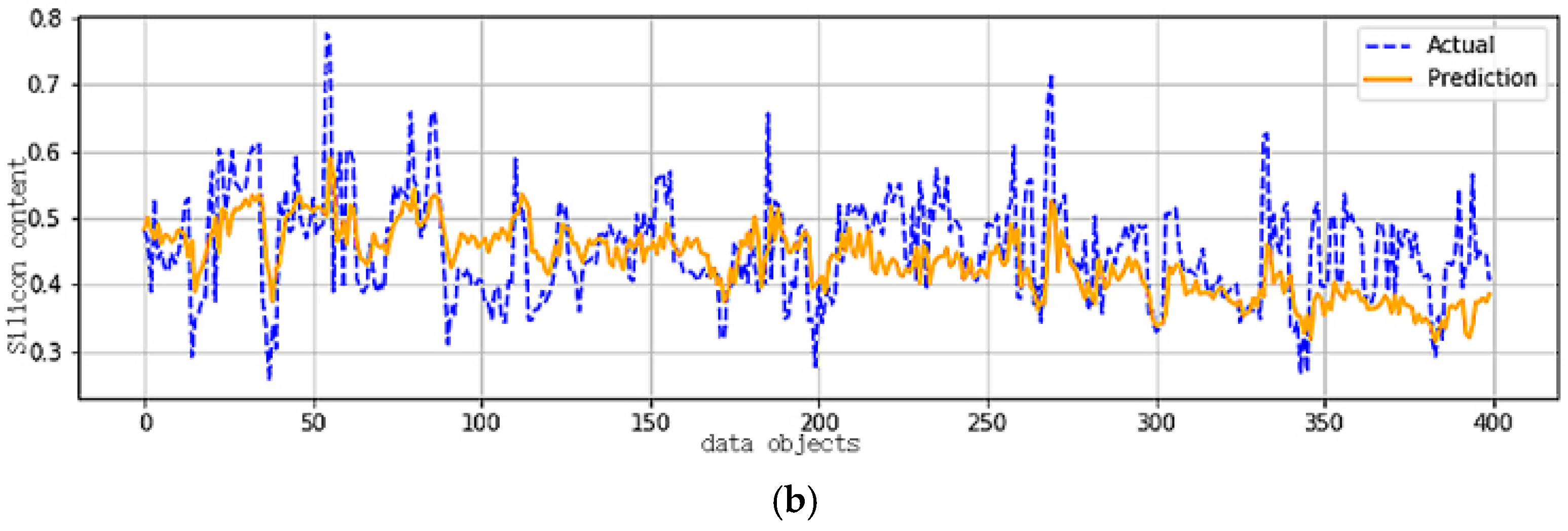
	3 (Figure 4)	0.0043	0.0047	87.93%	87.75%
	4	0.0042	0.0053	88.49%	84.25%
	5	0.0046	0.0047	86.55%	87.50%
$R_a$	1	0.0042	0.0055	88.06%	83.25%
	2	0.0040	0.0054	89.17%	83.50%
	3 (Figure 5)	0.0042	0.0057	88.89%	82.25%
	4	0.0045	0.0057	86.67%	81.50%
	5	0.0048	0.0052	87.36%	84.25%

(tests with the same test number share the same validation set). MSE and Hit are calculated as

$$MSE={\displaystyle \frac{1}{n}}{{\displaystyle \sum }}_{i=1}^n{\left({\widehat{y}}_i-y_i\right)}^2,$$

$$Hit={\displaystyle \frac{100\%}{n}}\left|\right\{{\widehat{y}}_i|\left|{\widehat{y}}_i-y_i\right|\le 0.1\}|$$

.

From Table 4, models trained with $R_r$ achieve better performance than those trained with $R_a$. Specifically, the training set results are almost the same (MSE about 0.043, Hit about 88%). However, the situation is different for the test set. The average Test_MSE and Hit for $R_r$ are 0.0049 and 86.3%, respectively, while 0.0055 and 82.9% for $R_a$. Compared with $R_a$, the Test_MSE decreases by 10.9% and Hit increases by 4.1%.

For further analysis, we selected the most representative test, i.e., test number 3, as shown in Figure 5 and Figure 6, for observation and comparison. For the training set, the figures are almost the same. However, for the test set, models trained based on $R_a$ fail to track the change in silicon content once the time point exceeds 300, whereas the models trained based on $R_r$ exhibit superior performance and effectively capture the trend of silicon content.

Through the above analysis, it is shown that the priority-optimal reduct retains more precise and relevant information than the classical reduction sets, and the related models demonstrate stronger generalization abilities. Therefore, the attribute reduction algorithm based on recursion proves to be practical in real-world applications.

5. Conclusions

In this study, we introduced a new definition of the priority-optimal reduct for complex industrial processes within rough set theory. Based on this, a recursive attribute reduction algorithm was developed. As the first recursive construction in the history of rough sets, it has important research value. Moreover, the results of experiments on silicon content prediction in a blast furnace demonstrate the effectiveness of our algorithm under complex blast furnace conditions.

Our work successfully applied the new attribute reduction to the feature selection of hot metal silicon content data from the blast furnace. In addition to the description of prior knowledge, the characteristics of the data itself should also be considered. Since the data are numerical, a discernibility relation that relies on discrete data may introduce quantization error. Thus, further investigation of tolerance relations, fuzzy relations, or a new discernibility relation is expected to yield better performance for this problem.

It should be noted that the performance of the proposed algorithm in practical applications heavily depends on a reasonable priority sequence, which is usually derived from experiential knowledge or mechanism analysis results. Consequently, there exists a potential overfitting risk when applying it to specific domain datasets. We leave a more robust priority sequence determination method to future work.

References

- Taher, D.I.; Abu-Gdairi, R.; El-Bably, M.K.; El-Gayar, M.A. Decision-making in diagnosing heart failure problems using basic rough sets. AIMS Math. 2024, 9, 21816–21847. [Google Scholar] [CrossRef]
- Zhang, Q.; Xie, Q.; Wang, G. A survey on rough set theory and its applications. CAAI Trans. Intell. Technol. 2016, 1, 323–333. [Google Scholar] [CrossRef]
- Yin, L.; Cao, K.; Jiang, Z.; Li, Z. RA-MRS: A high efficient attribute reduction algorithm in big data. J. King Saud Univ.-Comput. Inf. Sci. 2024, 36, 102064. [Google Scholar] [CrossRef]
- Qin, L.; Wang, X.; Yin, L.; Jiang, Z. A distributed evolutionary based instance selection algorithm for big data using Apache Spark. Appl. Soft Comput. 2024, 159, 111638. [Google Scholar] [CrossRef]
- Akram, M.; Ali, G.; Alcantud, J.C.R. Attributes reduction algorithms for m-polar fuzzy relation decision systems. Int. J. Approx. Reason. 2022, 140, 232–254. [Google Scholar] [CrossRef]
- Liu, G.; Feng, Y. Knowledge granularity reduction for decision tables. Int. J. Mach. Learn. Cyber. 2022, 13, 569–577. [Google Scholar] [CrossRef]
- Yin, L.; Qin, L.; Jiang, Z.; Xu, X. A fast parallel attribute reduction algorithm using Apache Spark. Knowl.-Based Syst. 2021, 212, 106582. [Google Scholar] [CrossRef]
- Xie, X.; Gu, X.; Li, Y.; Ji, Z. K-size partial reduct: Positive region optimization for attribute reduction. Knowl.-Based Syst. 2021, 228, 107253. [Google Scholar] [CrossRef]
- Turaga, V.K.H.; Chebrolu, S. Rapid and optimized parallel attribute reduction based on neighborhood rough sets and MapReduce. Expert Syst. Appl. 2025, 260, 125323. [Google Scholar] [CrossRef]
- Kumar, A.; Prasad, P.S.V.S.S. Enhancing the scalability of fuzzy rough set approximate reduct computation through fuzzy min–max neural network and crisp discernibility relation formulation. Eng. Appl. Artif. Intell. 2022, 110, 104697. [Google Scholar] [CrossRef]
- Sowkunta, P.; Prasad, P.S.V.S.S. MapReduce based parallel fuzzy-rough attribute reduction using discernibility matrix. Appl. Intell. 2022, 52, 154–173. [Google Scholar] [CrossRef]
- Xu, W.; Yuan, K.; Li, W.; Ding, W. An Emerging Fuzzy Feature Selection Method Using Composite Entropy-Based Uncertainty Measure and Data Distribution. IEEE Trans. Emerg. Top. Comput. Intell. 2023, 7, 76–88. [Google Scholar] [CrossRef]
- Sang, B.; Chen, H.; Yang, L.; Li, T.; Xu, W. Incremental Feature Selection Using a Conditional Entropy Based on Fuzzy Dominance Neighborhood Rough Sets. IEEE Trans. Fuzzy Syst. 2022, 30, 1683–1697. [Google Scholar] [CrossRef]
- Ji, X.; Li, J.; Yao, S.; Zhao, P. Attribute reduction based on fusion information entropy. Int. J. Approx. Reason. 2023, 160, 108949. [Google Scholar] [CrossRef]
- Fontes, D.O.L.; Vasconcelos, L.G.S.; Brito, R.P. Blast furnace hot metal temperature and silicon content prediction using soft sensor based on fuzzy C-means and exogenous nonlinear autoregressive models. Comput. Chem. Eng. 2020, 141, 107028. [Google Scholar] [CrossRef]
- Nistala, S.H.; Kumar, R.; Parihar, M.S.; Runkana, V. metafur: Digital Twin System of a Blast Furnace. Trans. Indian. Inst. Met. 2024, 77, 4383–4393. [Google Scholar] [CrossRef]
- Jiang, K.; Jiang, Z.; Xie, Y.; Pan, D.; Gui, W. Prediction of Multiple Molten Iron Quality Indices in the Blast Furnace Ironmaking Process Based on Attention-Wise Deep Transfer Network. IEEE Trans. Instrum. Meas. 2022, 71, 2512114. [Google Scholar] [CrossRef]
- Liu, C.; Tan, J.; Li, J.; Li, Y.; Wang, H. Temporal Hypergraph Attention Network for Silicon Content Prediction in Blast Furnace. IEEE Trans. Instrum. Meas. 2022, 71, 2521413. [Google Scholar] [CrossRef]
- Li, J.; Yang, C.; Li, Y.; Xie, S. A Context-Aware Enhanced GRU Network with Feature-Temporal Attention for Prediction of Silicon Content in Hot Metal. IEEE Trans. Ind. Inf. 2022, 18, 6631–6641. [Google Scholar] [CrossRef]
- Wang, W.; Huang, B.; Wang, T. Optimal scale selection based on multi-scale single-valued neutrosophic decision-theoretic rough set with cost-sensitivity. Int. J. Approx. Reason. 2023, 155, 132–144. [Google Scholar] [CrossRef]
- Shu, W.; Xia, Q.; Qian, W. Neighborhood multigranulation rough sets for cost-sensitive feature selection on hybrid data. Neurocomputing 2023, 565, 126990. [Google Scholar] [CrossRef]
- Yang, J.; Kuang, J.; Liu, Q.; Liu, Y. Cost-Sensitive Multigranulation Approximation in Decision-Making Applications. Electronics 2022, 11, 3801. [Google Scholar] [CrossRef]
- Su, H.; Chen, J.; Lin, Y. A four-stage branch local search algorithm for minimal test cost attribute reduction based on the set covering. Appl. Soft Comput. 2024, 153, 111303. [Google Scholar] [CrossRef]