Article

Generating Synthetic Sperm Whale Voice Data Using StyleGAN2-ADA

1
Youth Research Institute, Saint Petersburg Electrotechnical University “LETI”, 197022 Saint Petersburg, Russia
2
Computer-Aided Design Department, Saint Petersburg Electrotechnical University “LETI”, 197022 Saint Petersburg, Russia
*
Authors to whom correspondence should be addressed.
Big Data Cogn. Comput. 2024, 8(4), 40; https://doi.org/10.3390/bdcc8040040
Submission received: 8 February 2024 / Revised: 30 March 2024 / Accepted: 2 April 2024 / Published: 3 April 2024

Abstract

:
The application of deep learning neural networks enables the processing of extensive volumes of data and often requires dense datasets. In certain domains, researchers encounter challenges related to the scarcity of training data, particularly in marine biology. In addition, many sounds produced by sea mammals are of interest in technical applications, e.g., underwater communication or sonar construction. Thus, generating synthetic biological sounds is an important task for understanding and studying the behavior of various animal species, especially large sea mammals, which demonstrate complex social behavior and can use hydrolocation to navigate underwater. This study is devoted to generating sperm whale vocalizations using a limited sperm whale click dataset. Our approach utilizes an augmentation technique predicated on the transformation of audio sample spectrograms, followed by the employment of the generative adversarial network StyleGAN2-ADA to generate new audio data. The results show that using the chosen augmentation method, namely mixing along the time axis, makes it possible to create fairly similar clicks of sperm whales with a maximum deviation of 2%. The generation of new clicks was reproduced on datasets using selected augmentation approaches with two neural networks: StyleGAN2-ADA and WaveGan. StyleGAN2-ADA, trained on an augmented dataset using the axis mixing approach, showed better results compared to WaveGAN.

1. Introduction

Deep neural networks possess the capacity to extract features and detect intricate nonlinear correlations across diverse datasets. The advent of convolutional neural networks (CNNs) [1] has facilitated the utilization of neural networks in computer vision, encompassing applications in image classification, object detection, and image segmentation. In addition, neural networks are now commonly employed in non-photorealistic rendering (NPR) [2], including the generation of original images for tasks such as robotic painting [3] and other techniques such as neural style transfer (NST).
Neural networks are capable of processing many types of data other than images, including the generation of text using large language models like ChatGPT. The use of neural networks in natural language processing (NLP) has increased significantly in recent decades. Recent developments include the rise of models like BERT [4] and GPT-3 [5], which have further pushed the boundaries of language understanding and generation. These models leverage large-scale training on text data to achieve remarkable levels of fluency and coherence in the generated text. For further reading on natural language processing, the reader is encouraged to refer to [6,7].
Deep neural networks are frequently employed to analyze audio data for sound recognition and classification, particularly in the context of animal and environmental sound discrimination [8,9]. Neural convolutional networks, in particular, are commonly used for this purpose. Furthermore, neural networks find applications in medicine for the identification of cough sounds and many other related tasks [10,11]. Furthermore, neural networks are broadly used for speech synthesis applications, e.g., speech assistants or gaming avatars [12,13,14]. They are also utilized in the generation of audio data, including biological sounds and music produced by various instruments, e.g., drums or piano [15,16]. The production of animal vocalizations holds significant importance for studying their behavioral patterns and communication methods, as well as for using these vocalizations in technical applications. The field of audio generation has been extensively explored by numerous researchers. The possibility to convert an audio recording into a visual representation has enabled the application of feature extraction methods commonly employed for image classification [17,18]. For instance, Dhariwal et al. [19] have devised Jukebox, a model specifically designed to generate singing in the raw audio domain. Similarly, van den Oord et al. [20] introduced WaveNet, a deep generative model with the ability to operate at the waveform level, thereby enabling the production of authentic human speech and select musical segments. Finally, Chris Donahue developed WaveGAN [15], an approach that utilizes generative adversarial networks (GANs) for unsupervised synthesis of raw audio signals.
A key objective within the field of sound generation is the generation of vocalizations emitted by diverse animal species. The reproduction of such vocalizations plays a significant role in the examination of behavioral patterns and communication modalities exhibited by the animals and can be a perfect basis for biologically inspired technical solutions. Regarding animal sound classification and recognition, a prevalent issue is the scarcity of audio data [21]. An attempt to address this problem was made by Axel-Christian Guei et al. [22], who introduced a novel methodology for generating ECOGEN bird sounds. By employing the VQ-VAE2 architecture, the authors generated new spectrograms that can subsequently be converted back into a digital audio signal. In a recent study [23], E Kim et al. proposed a GAN-based animal audio data augmentation scheme. The authors generated new audio data using DualDiscWaveGAN and then assessed the reliability of the resulting virtual data, selecting data with high scores for augmentation. Therefore, the main goal of such research is to address the lack of audio data by using deep learning networks to enrich existing biological audio data samples.
Certain animal species, e.g., whales, are either rare or possess vocalizations that are challenging to record due to their low-accessible habitats. To record acoustic data in aquatic environments, special devices called hydrophones are commonly used. Moreover, the large-scale collection of data over extended periods, spanning several years for instance, necessitates the employment of autonomous and semi-autonomous systems that operate consistently in the habitats of the animals under study [24]. These systems include tethered buoy arrays [25,26], tags or recording devices attached to the whales [27], aquatic drones with varying levels of autonomy [28], and aerial drones equipped with hydrophones [29]. Even with all this equipment, collecting audio data from a single group of whales can take several years, and the amount of data may still be insufficient. To address this problem, in the current study, we propose a reliable technique to generate synthetic whale audio data using a limited initial dataset.
The main contributions of this work are as follows:
  • We introduce an approach to reduce the scarcity of whale audio data by analyzing its spectral characteristics.
  • We describe a method for producing synthetic acoustic data for sperm whales using the StyleGAN2-ADA network.
  • Several experiments conducted on authentic sperm whale audio datasets show the high resemblance between the augmented and synthetically created data derived using the proposed approach, in contrast to other considered data augmentation methods.
The remainder of this paper is structured as follows. Section 2 provides a review and description of the primary methods for augmenting and generating audio data. Section 3 presents the proposed data augmentation method, along with the architecture and operational principles of the GAN employed for generating synthetic sound data related to whales. The experimental findings and a comparative analysis of the proposed methodologies are given in Section 4. Finally, Section 5 concludes this paper.

2. Related Works

One of the main problems faced by researchers working with neural networks is the insufficient amount of training data, the lack of which can lead to overfitting. In cases where real training data are deficient, different augmentation methods are employed [30,31]. The primary concept behind data augmentation is to modify one or more attributes of the original sample by a small increment to generate a novel, marginally altered data sample. Quite frequently, augmentation is applied to images since the problem of a limited dataset often arises when solving image processing problems [32]. Traditional image augmentation approaches involve employing a mix of such affine transformations like scaling, shearing, rotating, or modifying colors [33]. Nevertheless, more intricate transformations have also been suggested recently, like occluding regions of an image [34], blending multiple images [35], or introducing noise to images [36].
Augmentation of sound data is an important stage in the formation of datasets for training neural networks in the field of sound processing. The goal of this process is to create similar, but not identical, audio data to improve the model’s generalization ability and provide more information in situations where sufficient natural data may not be available. It is important to note that the content of an audio file can be represented in different ways, which, in turn, affects the type of augmentation method that can be applied [17]. For example, there are augmentation methods that are applied to the waveform of a signal. These include changing the pitch [37], increasing/decreasing the volume of the signal, changing the speed (speeding up or slowing down the original signal), adding random noise, silence, mixing the signal with background sounds from different types of acoustic scenes [38], adding reverb [39,40], time shift (right or left), etc.
On the other hand, when an audio signal is represented as a spectrogram or mel-frequency cepstral coefficients (MFCCs), it becomes feasible to employ augmentation methods that are typically used for images. Methods like random cropping, time shifting, pitch shifting, and spectrogram warping can be especially beneficial. They help the model learn to be more invariant to such transformations and improve performance, especially in the case of a limited training dataset. A fairly popular augmentation method applicable to spectrograms is SpecAugment [41]. SpecAugment is a data augmentation method applied to the input data of a neural network, which involves masking along both the time and frequency axes of the mel-frequency cepstral coefficients (MFCCs). To facilitate the extraction of pertinent features by the network and bolster its resilience against temporal deformations, limited frequency information loss, and minor speech segment loss, the authors use the following types of mel-spectrogram deformations:
  • Time warping the sparse image. A logarithmic spectrogram is viewed as an image, where the time axis is horizontal and the frequency axis is vertical. A random point along the horizontal line passing through the center of the image within a certain range is warped either to the left or right by a randomly chosen distance.
  • Frequency masking involves masking a range of consecutive mel-frequency channels. The number of channels to be masked is first chosen randomly, and then the starting point for the masking is selected.
  • Time masking involves masking a range of sequential time steps. Similar to frequency masking, the number of time steps and the starting point for the masking are chosen randomly. Additionally, there is an upper bound on the width of the time mask.
Certain augmentation methods involve the summation of two random mel spectrograms of an identical class to generate a novel spectrogram [17]. For instance, Shengyun Wei et al. [42] used mixed-shape data augmentation on a time-frequency representation in the input space to train a convolutional recurrent neural network (CRNN). In [43], the authors described VTLP (Vocal Tract Length Perturbation), a method that distorts spectrograms by introducing random linear changes along the frequency axis. The central idea is not to eliminate differences but to add some variation to the audio. This can be achieved by normalizing to a specific value instead of a standard mean.
Data generation methods can also be constructed as augmentation techniques. Quite often, models based on generative adversarial networks (GANs) are employed to synthesize audio data. For example, WaveGAN represents an audio generation method based on the DCGAN [15] architecture but incorporates a customized 1 × 25 convolution operation instead of the standard 5 × 5 convolution. WaveGAN is explicitly designed for the generation of realistic audio data. It exhibits a wide range of applications and demonstrates high efficiency in audio synthesis tasks. Another GAN used for generating audio from synthesized data spectrograms is SpecGAN [15]. In comparison to WaveGAN, this approach exhibits lower performance. A significant drawback of GAN models is the random generation of output data, leading to an unregulated expansion of training data, which may have no effect on classifier training or even weaken it when working with small datasets. To address this issue, we propose a new method for synthesizing sperm whale signals that maximizes the preservation of the spectral characteristics of the original signal.
Thus, the following problems within the studied area can be identified:
  • Problems with training neural networks with small sizes of training samples.
  • The limited number of methods for augmenting sound data.
  • The area of generation of sound signals (including bio-similar ones) has been poorly studied in small samples.

3. Materials and Methods

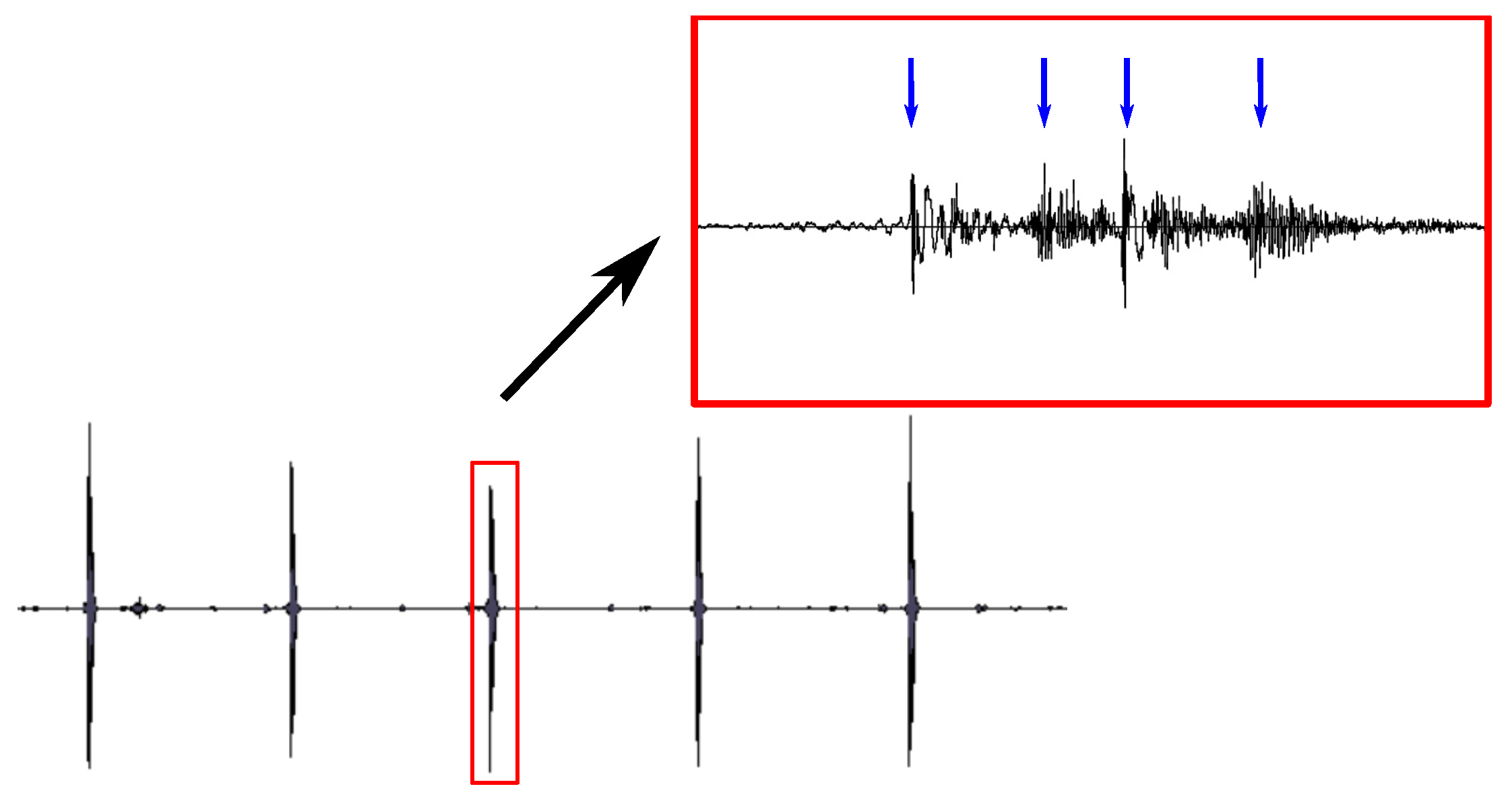
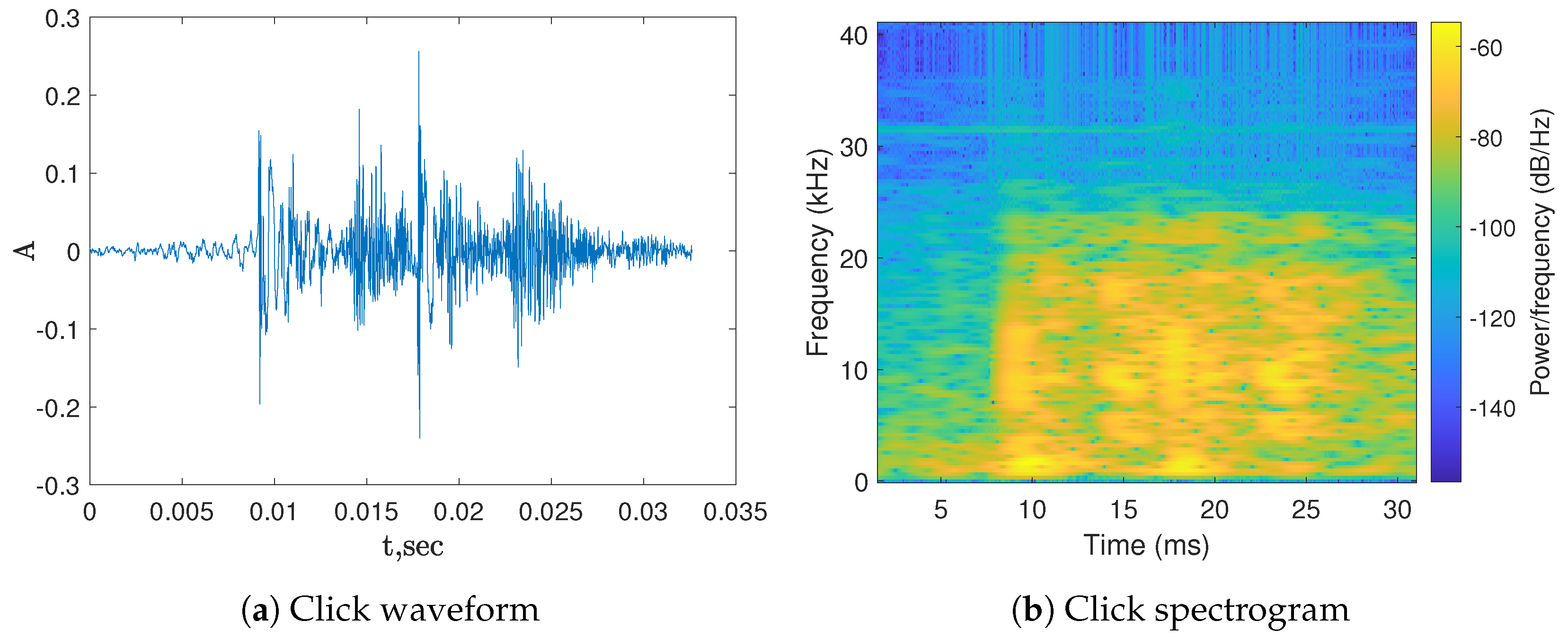
3.1. Sperm Whale Clicks

The sperm whale (cachalot) was chosen as a subject for this study among various marine mammals because of the unique characteristics of the sounds it makes. Sperm whales produce a series of single, broadband clicks that are used for echolocation, allowing the whales to find prey and navigate in the darkness of the deep ocean [44,45], as well as for communication. Each click has a multipulse structure, comprising an intense first pulse followed by several additional pulses (Figure 1).
The multipulse click is the result of the reverberation of the initial pulse in the spermaceti organ of the whale [46,47]. From the clicks, “codes” can be compiled—sequences of clicks with a fixed structure of relative intervals between clicks that have been identified as fundamental communicative units. It is known that sperm whales are divided into clans. Scientists distinguish clans depending on the dialect in which the sperm whales click [48,49,50]. However, it is still unknown whether the codes differ only in the absolute intervals between clicks, whether the spectral features of the clicks of the codes carry information, and whether the frequency of individual clicks in the codes matters.

3.2. Augmentation of Sperm Whale Clicks

In this research, two different approaches for audio data augmentation were employed. The first approach involved various traditional augmentation methods, which were applied to the original signal:
  • Changing the signal speed within the range of 0.8 to 1.2 compared to the original signal, implemented using the MATLAB function stretchaudio(S,k). The initial signal (S), its length, and the parameter for changing the audio speed (k) are transmitted as parameters.
  • Shifting the signal pitch within the range of − 3 to 3 semitones, implemented using the MATLAB function shiftpich(S,k). As parameters, the initial signal and the number of semitones for the shift (k) are passed to the function.
  • Changing the signal volume within the range of −3 to 3 dB. The new signal S n e w is obtained from the original signal S multiplied by the amplification factor, where k is the required amount of dB: S n e w = S · 10 k 20 .
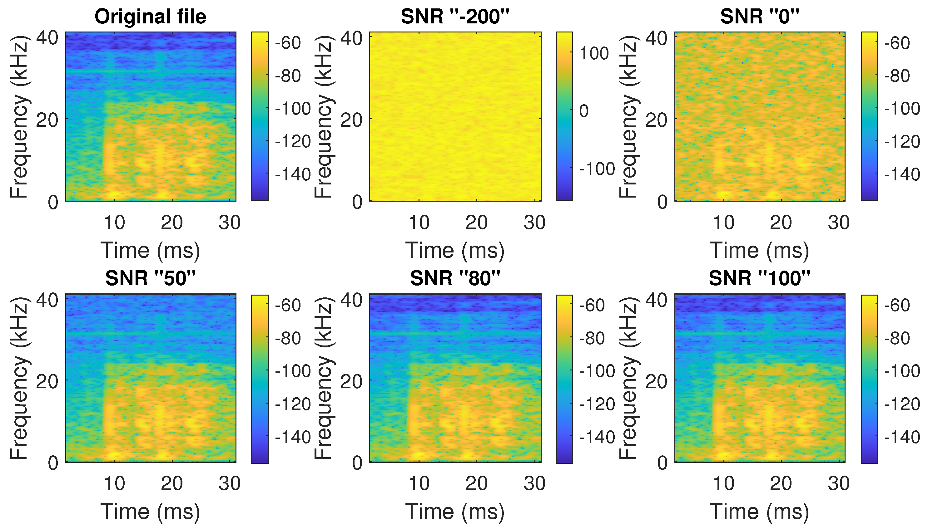
  • Addition of random noise to the signal, with a signal-to-noise ratio (SNR) between 50 and 100, implemented using the MATLAB function awgn(S,snr). The parameters include the original signal (to which noise is to be added) and the signal-to-noise ratio (SNR) (to modulate the intensity of the added noise). The SNR parameter was selected to ensure that the operation did not distort the original signal. Sometimes, it is necessary to adjust the SNR parameter in such a way that it does not distort the original signal. Figure 2 shows an example of adding noise to the original signal with different original signal-to-noise ratios.
  • Time shifting of certain elements within the range of −0.0001 to 0.0001 s. To implement this augmentation approach, some elements of the original signal are swapped with neighboring ones that are within a range satisfying the conditions of a given interval.
The augmentation approach we used in our study creates several augmented signals from the original one. Each of the five transformations described earlier can be applied to a signal with some probability. Thus, the parameters for augmentation are set randomly within specified intervals, and the methods that will be applied are also randomly selected. A more detailed description of the operation of the augmentation algorithm using classical transformations is described in the pseudocode given in Algorithm 1.
Algorithm 1: Augmentation approach used in classical methods
Bdcc 08 00040 i001
One of the original signals, presented in the form of a one-dimensional array, is the input for the augmentation algorithm, along with information about the length of the signal, which is equal to the number of points in the array. The desired number of iterations to complete the augmentation loop is set by the user, so the number of augmented signals received can be arbitrary. Next, the algorithm generates a random integer from the interval [1; 3]. If the randomly generated number is 1, then one of the five transformations described earlier is applied to the signal. This procedure is repeated for each of the described transformations, with equal chances of application. The parameters for changing the signal at each stage are also set with random values within the previously established intervals. At the end of the cycle, the augmented signal is saved. The next iteration re-introduces the random values. The second approach involves creating a new signal by combining segments from several source files, S i g 1 and S i g 2 . The idea of this approach is to take two source signals and swap horizontal or vertical sections of the spectrogram image. For example, if there are three parts, two segments from the first file and one segment from the second file can be assembled to form a new file from these three parts. The original signal is converted from a waveform to a spectrogram using a short-time Fourier transform (STFT), and the result is written into a two-dimensional array for each file, S t f t 1 and S t f t 2 . Then, the dividing points of the spectrograms are calculated both in time and frequency and recorded in the d A t variables. Knowing the division points, the selected parts of the arrays are swapped among themselves, and then the inverse Fourier transform is applied to the new sequences and written to the M i x F r e q S i g n a l or M i x S i g n a l array, depending on the type of change used for mixing. Algorithm 2 describes this approach in pseudocode.
The proposed approach uses two different types of mixing: mixing along the time axis (Figure 3) and mixing along the frequency axis (Figure 4). The audio file is converted into a spectrogram, where the X-axis represents time, and the Y-axis shows frequency values. In the case of temporary blending, the image is cut into fragments by vertical lines.
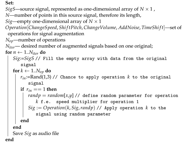
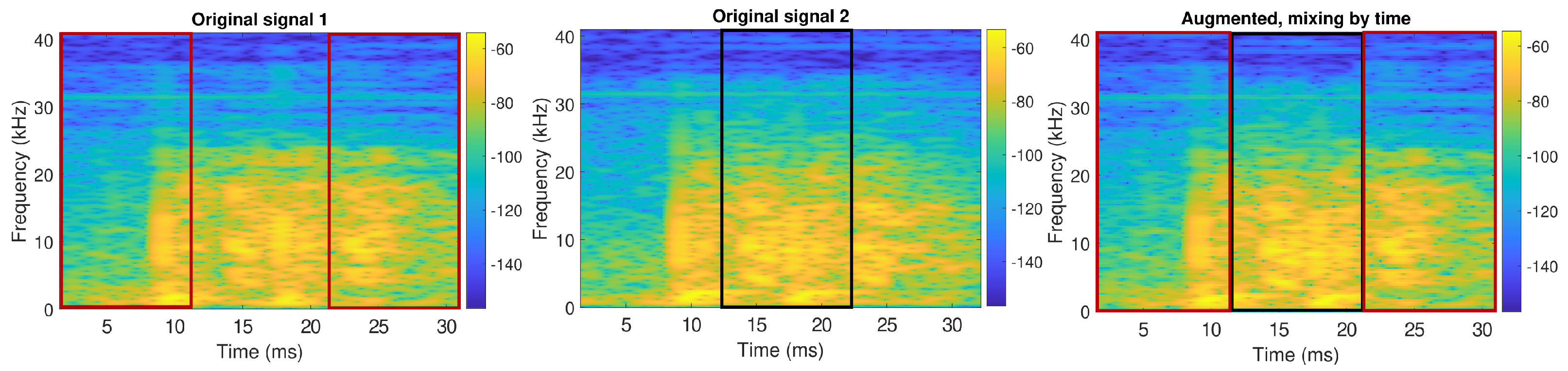
Algorithm 2: Augmentation approach used in mixing methods
Bdcc 08 00040 i002
In the case of mixing along the frequency axis, the spectrogram image is cut into fragments by vertical lines.

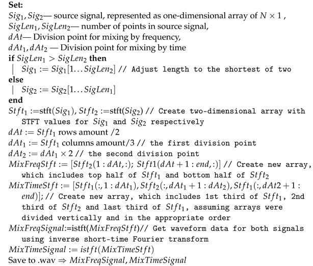
3.3. Deep Learning Models for Sperm Whale Audio Data Generation
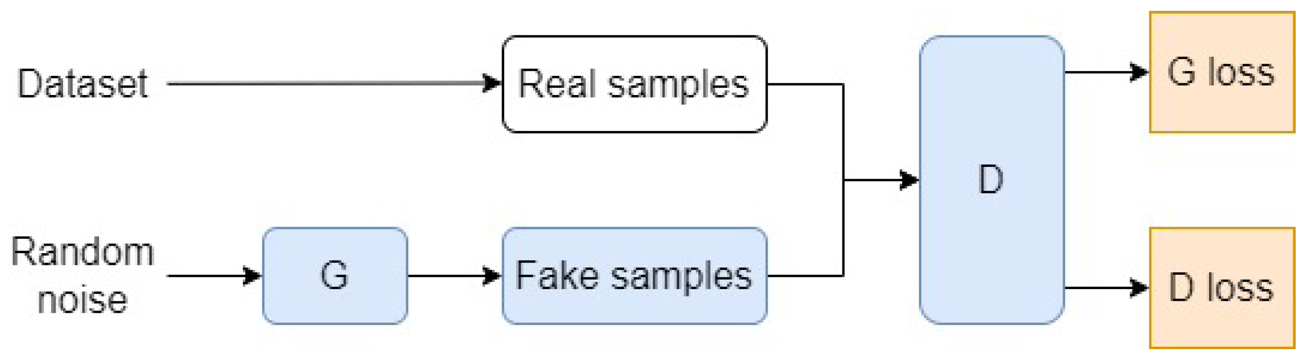
To generate sperm whale signals, in this study, we use two neural networks based on generative adversarial networks (GANs) (Figure 5).
Such neural networks consist of two main components: a generator and a discriminator. The generator creates images that can be visually similar to the real ones, while the discriminator tries to distinguish the real data from the generated ones. GAN training occurs through competition between the generator, which strives to produce increasingly realistic images, and the discriminator, which tries to distinguish synthetic images.
The first neural network under investigation is WaveGAN [15], an audio generation method that specializes in creating realistic audio data and has a wide range of applications. The second considered method is StyleGAN2-ADA [51]—a neural network that allows users to create fairly realistic images. In this study, StyleGAN2-ADA is used for the first time to generate audio data represented as spectrograms. The architecture and basic principles of operation of these neural networks are described below.

3.3.1. WaveGAN

WaveGAN is a type of generative adversarial network designed to produce raw audio signals rather than images or spectrograms. Its architecture is based on the DCGAN model, which uses a technique called transposed convolution to enhance the resolution of low-detail feature maps, creating higher-quality images. DCGAN is a direct extension of GAN, except that it explicitly uses convolutional and transponous convolutional layers in the discriminator and generator, respectively. In the case of WaveGAN, this transposed convolution operation is adapted to use longer 1D filters and increase the upsampling factor at each layer. These changes allow WaveGAN to possess the same characteristics in terms of parameters, operations, and output as the DCGAN but with additional audio sample capabilities. As DCGAN generates 64 × 64-pixel images, which equals only 4096 audio samples, the authors introduced an extra layer to the model, allowing it to produce 16,384 samples, equivalent to a bit over one second of audio at a 16 kHz sampling rate.
For the task of generating biological signals, it is necessary to create audio samples with a high sampling rate, which can be limited by WaveGAN. Therefore, in our work, we propose to use StyleGAN2-ADA with a generator that can generate high-resolution images.

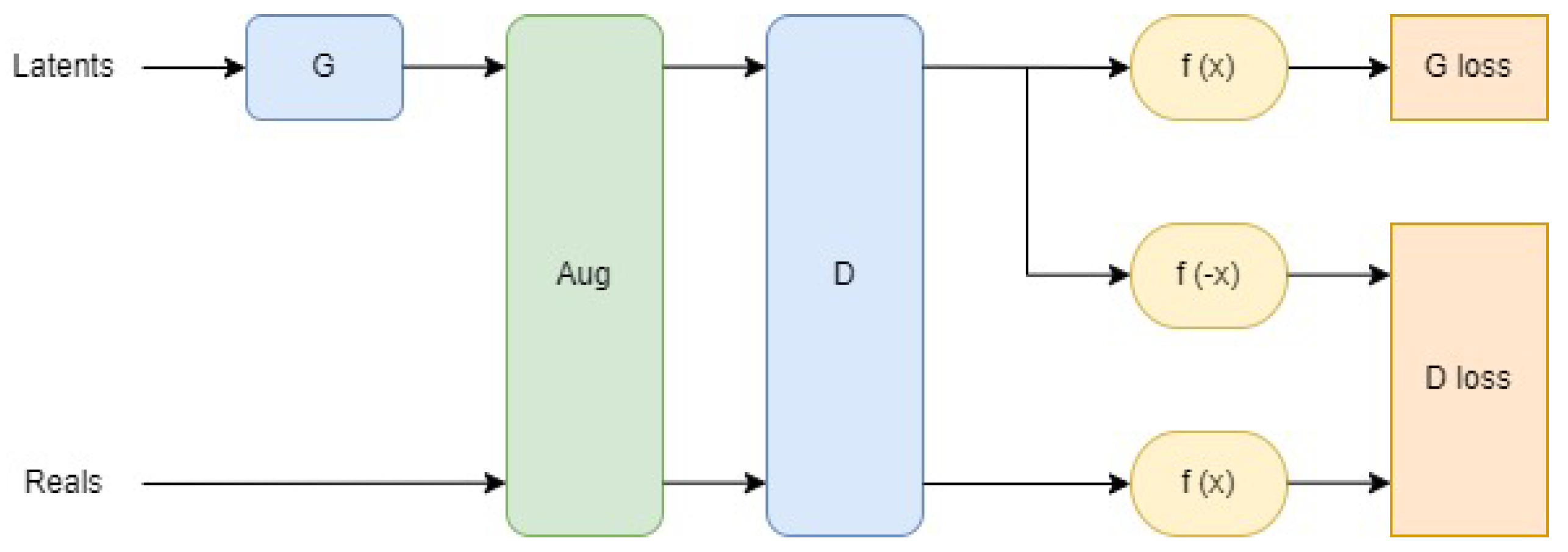
3.3.2. StyleGAN2-ADA

The idea of using the GAN architecture for sound generation can be traced back to SpecGAN [15]. To obtain audio from a generated spectrogram, the value of each pixel’s color is read, and the sum of the components is recorded in a 2D tensor, with one element corresponding to one pixel. The padding, which is the black part at the bottom, is removed, and the resulting tensor values are mapped back to the original spectrogram range. The audio waveform is obtained using the inverse_spectrogram function on the tensor, utilizing the same dataset parameters as when the audio was converted to spectrograms, and then saved using the w a v f i l e . w r i t e function.
StyleGAN2-ADA is a network based on the GAN architecture with two competing parts—the generator and discriminator—with the addition of an adaptive discriminator augmentation (ADA) mechanism, designed to lower the training divergence when working with limited datasets. The main idea of ADA is that all images shown to the discriminator go through a set of augmentations, so the discriminator never encounters the original images from the dataset. Thus, controlled augmentations of inputs can balance out the learning speed between the two networks. Other than this, no other changes were made to the structure.
Figure 6 shows the structure of StyleGAN2-ADA. The generator receives white noise and generates images. Both real and generated spectrograms go through the same augmentation pipeline before being fed into the discriminator. The discriminator gives a score to each image, and the results are used in the evaluation of the loss function for each network. Blue represents the training networks, yellow represents the evaluation of the loss function f ( x ) = l o g ( 1 1 + e x ) based on the discriminator outputs, green represents the application of augmentations, and orange represents the values of the loss function.
Each image goes through the augmentation pipeline, where each augmentation can be applied to each image with a probability p or skipped with a probability 1 p . To avoid manual adjustment of the parameter, the probability p changes based on the degree of overfitting. Overfitting is determined by the divergence of the discriminator outputs between the real and generated images, with the ideal scenario being that they are close to each other, indicating that the generated images are indistinguishable from the training set. Consequently, the more overfitted the network becomes, the farther apart the outputs become. The metric used to evaluate overfitting is expressed as
r t = E [ s i g n ( D t r a i n ) ] ,
where D t r a i n represents the discriminator outputs for the training set. This heuristic is chosen because it does not require a separate validation batch. After a certain number of minibatches, p is adjusted based on this heuristic, starting from 0 at the beginning of the training.
The network was trained using the Google Colab platform which is known to equipped with an NVIDIA Tesla T4 12GB GPU. The StyleGAN2-ADA PyTorch implementation [51] was employed for this study. The generated images were 256 × 256 pixels. While higher resolutions can still be used, it was determined that smaller resolutions are too restrictive and larger ones are too time-consuming. StyleGAN2-ADA offers various augmentation categories, such as pixel blitting, geometric transformations, color transforms, image-space filtering, additive noise, and cutout. It should be noted that the last three augmentations are more impactful than the first three. When applying augmentations, it was ensured that they do not affect the colors, as the generated spectrograms already lack ideal color coding from the audio-to-image conversion. Therefore, only pixel blitting and geometric augmentations were utilized, while the stronger augmentations were avoided to prevent slow conversion. In the case of the augmented datasets, our pre-trained networks were utilized to mitigate the occurrence of premature overfitting and extended conversion times. Training persisted until the discriminator had been presented with 132,000 images, with network snapshots captured every 12,000 images. At this juncture, most datasets exhibited relative stability, and further training was deemed less essential due to time constraints.

3.4. Metrics for Audio Data Evaluation

The following metrics were chosen to evaluate and compare the augmented and generated audio data:
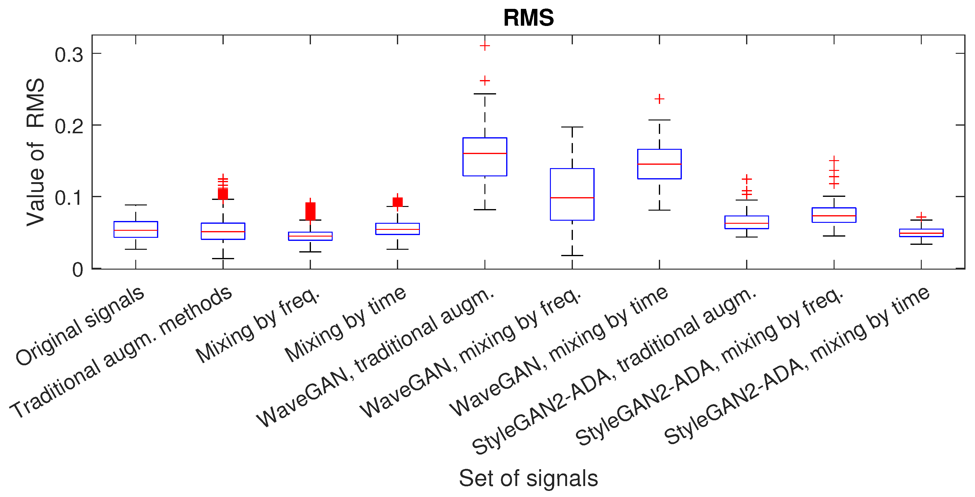
  • RMS: The root-mean-square value of the signal. This metric provides information about the effective signal energy and is more representative than a simple average amplitude value. The RMS is calculated using the following formula:
    R M S = 1 N n = 1 N | S n | 2 ,
    where S n is the value of the signal at the N-th point and N is the number of points in the signal.
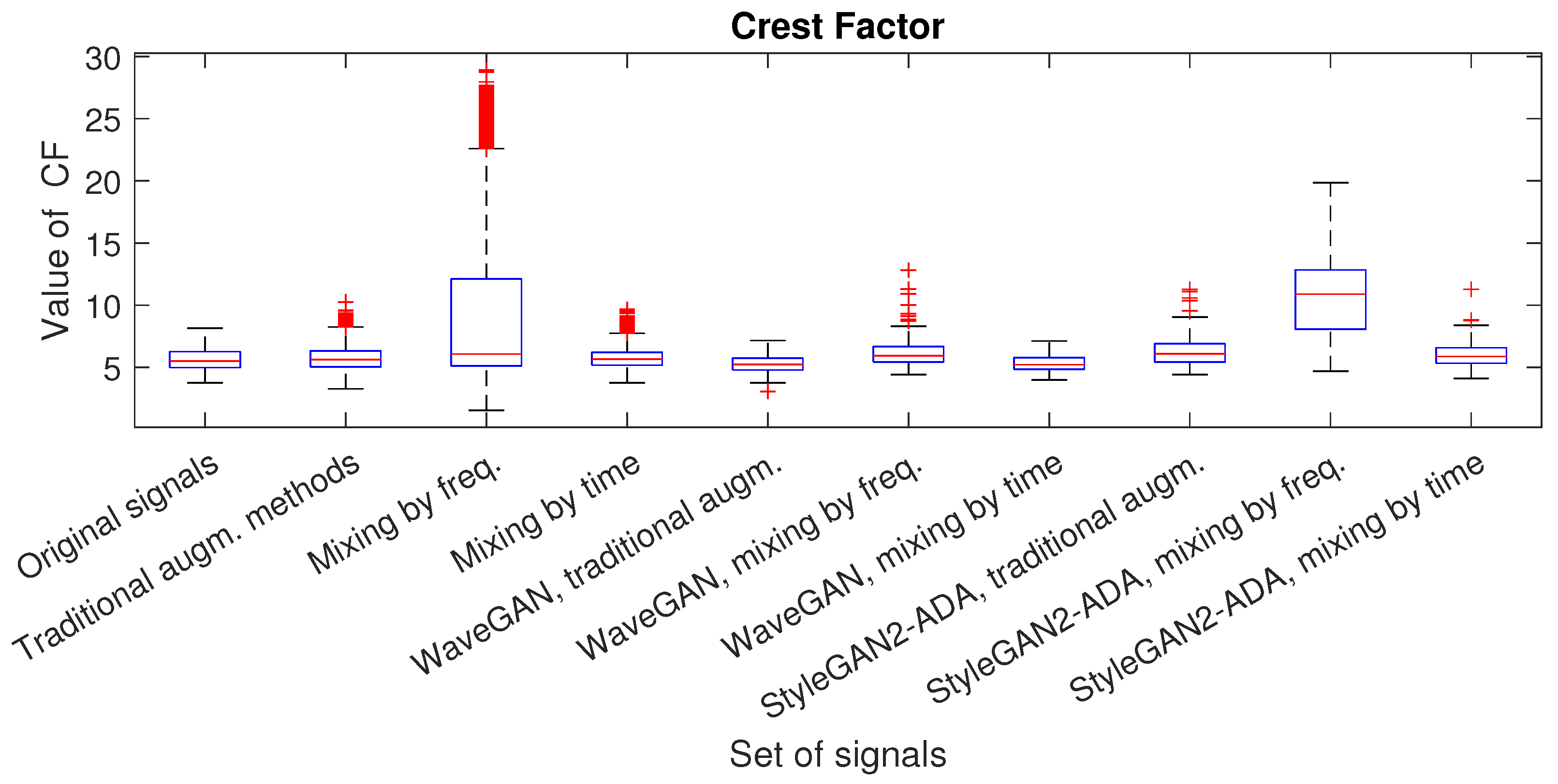
  • Crest factor: This metric allows one to detect failures that manifest themselves in changes in the peak frequency of the signal. High values of this metric mean that the signal contains short-term peaks or high-frequency pulses. The crest factor is calculated using the following formula:
    C F = S m a x R M S ,
    where S m a x is the maximum value of the signal.
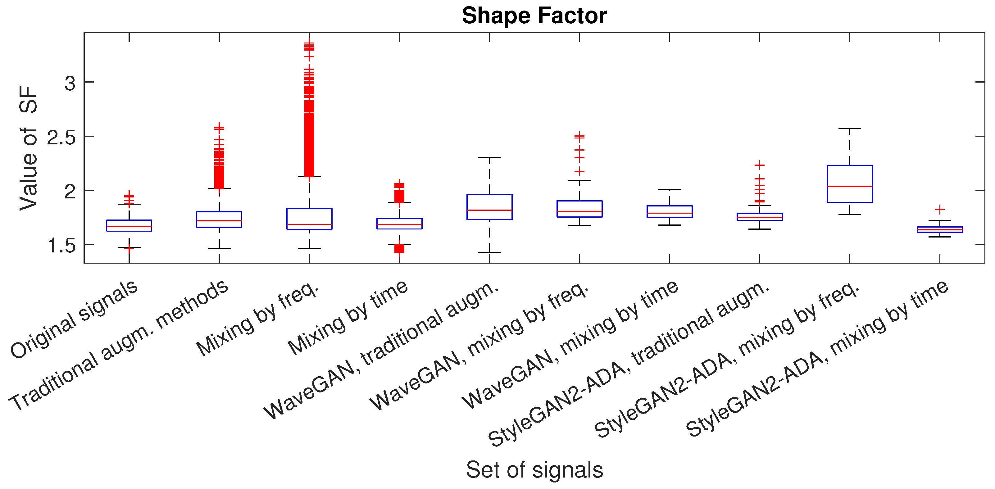
  • Shape factor: This metric evaluates the shape of a signal regardless of its size. The shape factor is calculated using the following formula:
    S F = R M S 1 N n = 1 N | S n |
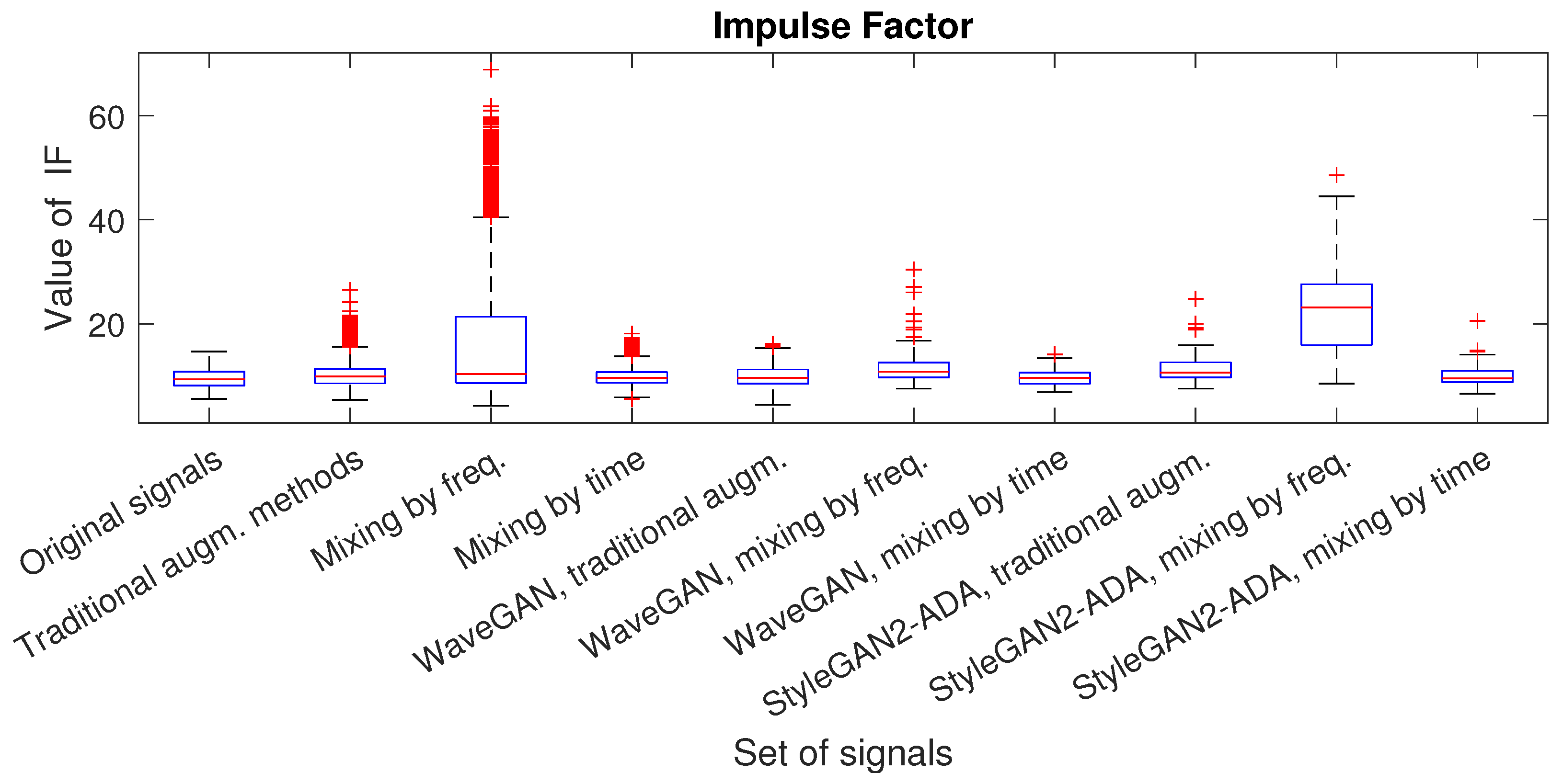
  • Impulse factor: This metric evaluates the sharpness of pulses or peaks in a signal. The impulse factor is calculated using the following formula:
    I F = S m a x 1 N n = 1 N | S n |
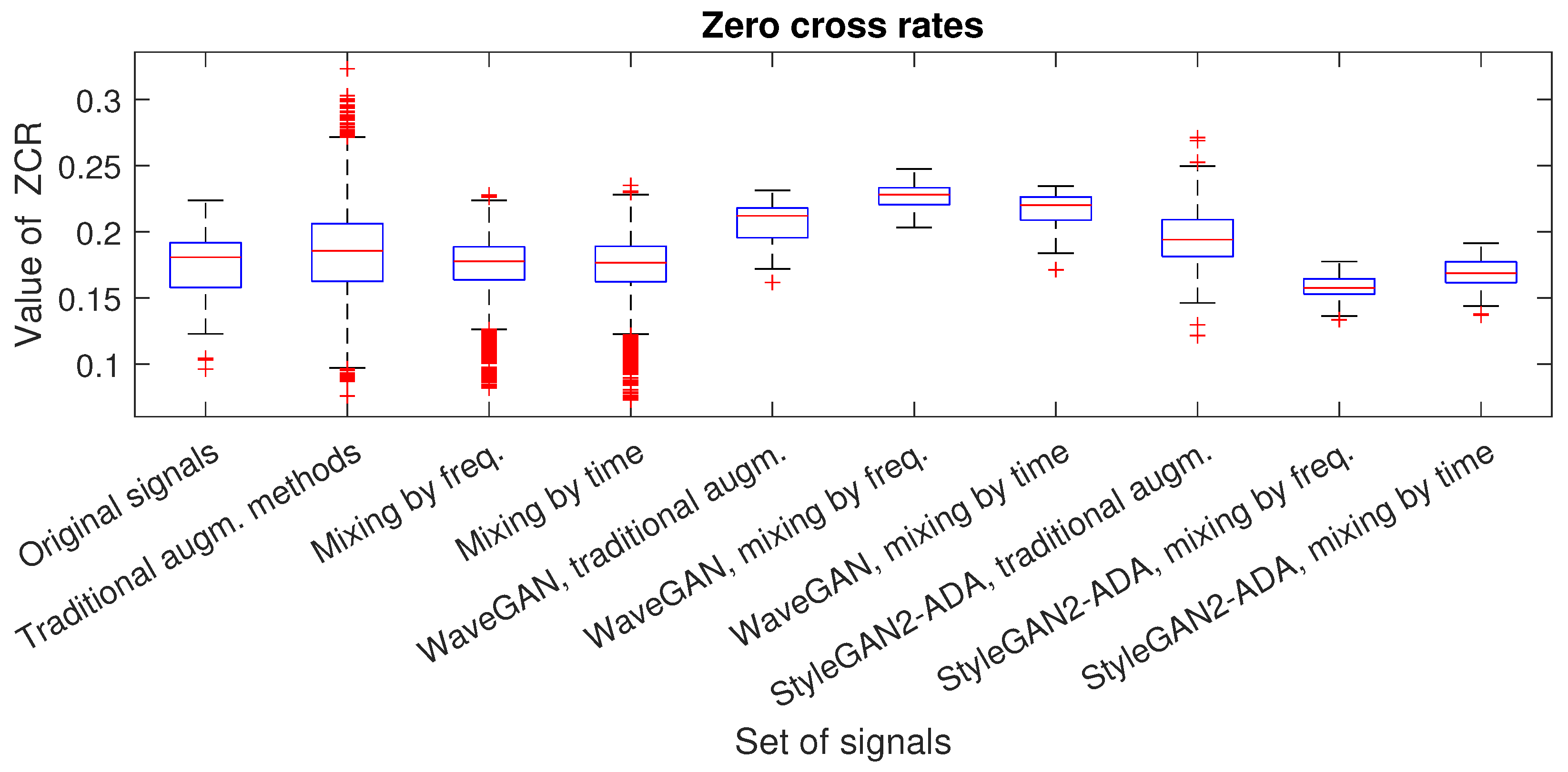
  • Zero-crossing rate: This metric shows how many times the signal crosses the amplitude value of “0” during the shown period, which indicates the smoothness of the signal.

4. Results

4.1. Dataset Description

The recordings of sperm whale clicks were obtained from the Watkins Marine Mammal Sound Database [52]. This large database contains samples of vocalizations from various marine mammals and is freely available. We selected a four-channel recording of the clicks produced by one tagged sperm whale from Dominica dated 21 September 1991. The file sampling frequency is 81,920 Hz. In the recording, the lonely clicks of a whale can be clearly heard, and there is the audible sound of a ship in the background. Therefore, the Savitzky–Golay [53] filter was applied for denoising purposes. While one of the most commonly used low-pass filters in signal processing is the moving average method, the Savitsky–Golay filter has proven itself effective in noise reduction for biological signals such as lung sounds [54] and ECG signals [55,56]. We tested several data smoothing methods (moving average, LOESS, LOWESS, and Gaussian filters), and the Savitsky–Golay filter showed the best results. This filter exhibited minimal phase shift compared to other filters. Individual whale clicks were then cut out and recorded into separate files, resulting in 81 separate chunks of sperm whale clicks that were used in our study as an example of a dataset with insufficient data. Figure 7 shows an example of one click that was cut out.
Sperm whale vocalizations are characterized by broadband, high-frequency short clicks. The duration of clicks in our study was around 0.03 s.Figure 7b shows that the frequencies we are interested in are within the range of 0.15 to 25 kHz. The spectrogram shows a band of about 31 kHz, which is either extraneous noise or a recording defect. In any case, this frequency does not distort the original signal.

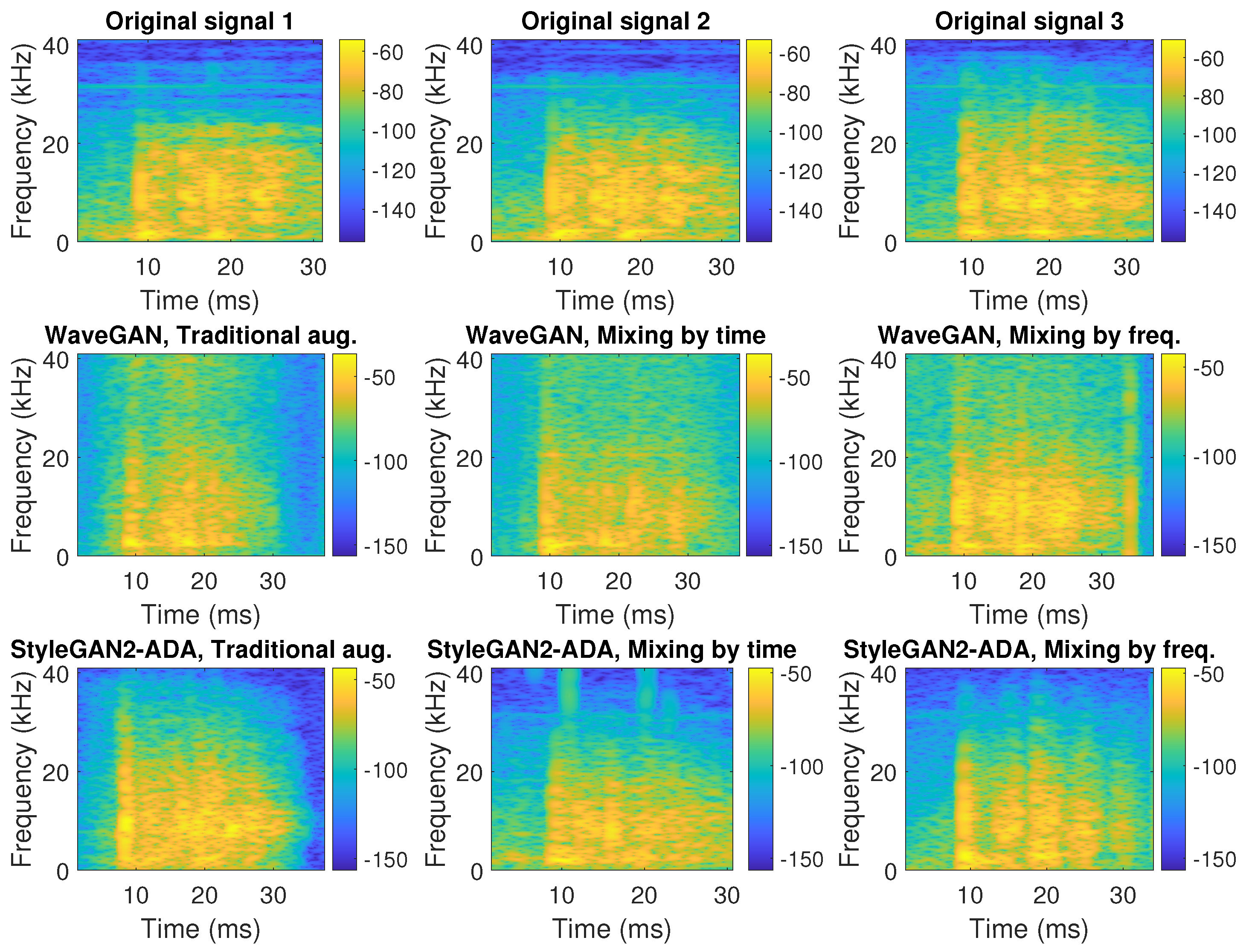
4.2. Data Augmentation and Generation Results with WaveGAN and StyleGAN2-ADA

First, we applied the augmentation algorithms, i.e., the classical approaches (Algorithm 1) and the method based on mixing parts of spectrograms (Algorithm 2). It was decided to apply each algorithm 81 times to each of the source files. Thus, the dataset obtained by applying each augmentation approach was equal in size to the datasets obtained previously. With 81 original files and combining fragments of each of them with all the others, 81 2 = 6561 new files were obtained for each of the three types of augmentation. The WaveGAN and StyleGAN2-ADA neural networks were trained on each augmented dataset. The main training parameters are given in Table 1.
After training, each neural network was used to generate 100 audio files for each augmented dataset. Examples of frequency representations of the augmented and generated sets for each investigated approach are shown in Figure 8.
Figure 8 shows that, on average, all files repeated the frequency range of the source files, i.e., the main frequencies are up to 25 kHz, and the multi-impulse nature of the signals is visible, as depicted by the vertical stripes on the spectrograms. WaveGAN is characterized by the addition of a high-frequency characteristic, which is visible from 20 kHz to 40 kHz (lighter areas). In files generated by StyleGAN2-ADA, such features are not that obvious.
Figure 9, Figure 10, Figure 11, Figure 12 and Figure 13 allow one to compare the chunks augmented and generated using WaveGAN and StyleGAN2-ADA with the metrics from Section 3.4. Figure 9 shows the RMS values of the signal. The obtained results show a strong deviation in the values for the files generated by WaveGan, approximately twice that of the values of the original files.
Figure 10 shows the values of the shape factor. This metric evaluates the shape of the signal regardless of its size. The figure shows that there were no strong deviations, but it is clear that for the augmented and generated files based on the mixing method along the frequency axis, the shape factor was overestimated and had many outliers. The same situation was observed for the impulse factor (Figure 11) and the crest factor (Figure 12).
Figure 13 shows the values of the zero-crossing rate, which indicates the smoothness of the signal. It can be seen in the figure that the files generated by WaveGAN have a smoother shape compared to the original files.
The results obtained using the augmentation methods showed good agreement with the original signals in terms of the spectral characteristics and selected metrics. Table 2 summarizes the average values of the generated and augmented files for each metric. The results presented in Table 2 should be interpreted as follows: the closer the dataset metric value is to that of the original signal, the more similar the signals. The percentage value indicates the deviation from the metric of the original signal, expressed as a percentage. The first row of the table shows the average values of the metrics for the original signals. The next three rows show the average metric values for the augmented data, followed by the average metric values for the data generated by the neural networks.
The deviation in the values of the metrics from the original signal may not be too small (about 0), as overly similar data would not provide enough diversity for training the neural network. But at the same time, the deviation should not be too large. We believe that a maximum deviation of 10–12% would be sufficient to ensure diversity in the data. As shown in Table 2, the best results for data augmentation were achieved by the mixing-by-time method. Nevertheless, the classical approaches also achieved good results. For the data generated by the neural networks, the best results were achieved by StyleGAN2-ADA when mixing by time. This is the only scenario where the deviation in the values of the metrics fell within the 10–12% range.

5. Conclusions and Discussion

In this study, we investigated methods for augmenting and generating synthetic sperm whale signals. Notably, the augmentation and generation of audio data derived from biological signals pose a persisting challenge that has yet to be comprehensively addressed. This paper aimed to clarify unresolved intricacies associated with sperm whale signal manipulation and generation and may be useful for researchers in the fields of cetacean communication, sonar construction, and signal processing.
We tested several augmentation methods, including a classical augmentation approach and a method involving the amalgamation of distinct segments of the spectrogram image. Using the mixing augmentation technique, the signal contents remained unchanged but were fragmented and reorganized, thereby preserving the key features observed in the original signals. All implemented augmentation methods offered flexibility for modification or joint utilization with other methods. All parameters were adjustable to accommodate different signal types or achieve diverse outcomes. Based on the obtained augmented datasets, new synthetic signals of sperm whales were generated using two neural networks: WaveGAN and StyleGAN2-ADA. The results showed that in terms of frequency characteristics, the generated files were similar to the original ones. However, the files generated by WaveGAN had an extra high-frequency component, which was not present in the samples generated by StyleGAN2-ADA. It should also be noted that both neural networks repeated the multipulse structure of a click. A comparison of the signals using metrics showed that among the augmentation methods, large deviations in the values of the crest factor (with an average increase of 57.22% relative to the original signal) and impulse factor (with an average increase of 71.15% relative to the original signal) were observed in the method mixing along the frequency axis. The augmentation method of mixing along the time axis yielded metric values closest to the original signals, with deviations ranging from 0.23 to 2%. Using a dataset based on this augmentation method, the metric values of the files generated by StyleGAN2-ADA were the closest to the original ones (with deviations of no more than 2%), making this augmentation method and neural network most suitable for the tasks of this study.
However, the proposed method possesses some limitations, and several problems typical of ANN-based solutions can be highlighted, e.g., the dependence on the training set and the need to retrain the network if the dialect of a group of whales is too different from the training set. Therefore, the direction of future research is the creation of whale signal generators that can generate entire phrases of an individual whale. Furthermore, we will study the generation of vocalizations of other cetaceans, which produce more harmonic sounds.
An area of ongoing research involves the creation of unique vocalizations (codes) based on generated clicks. This study may be useful in the tasks of identifying and classifying individual sperm whales, thereby contributing to a deeper understanding of cetacean communication patterns. The successful development of this study could potentially yield valuable insights into the nuanced language of cetaceans, paving the way for further discoveries in the field of marine mammal communication.

Author Contributions

Conceptualization, E.K. and D.B.; data curation, E.K. and A.K.; formal analysis, D.B.; investigation, T.S. and O.V.; methodology, E.K. and D.B.; project administration, E.K. and D.B.; resources, A.K. and D.B.; software, T.S. and O.V.; supervision, E.K.; visualization, T.S. and O.V.; writing—original draft preparation, E.K. and O.V.; writing—review and editing, T.S., A.K. and D.B. All authors have read and agreed to the published version of the manuscript.

Funding

This study was supported by the Russian Science Foundation (RSF), project 23-71-01084.

Data Availability Statement

The source codes of the augmentation algorithms and all datasets can be accessed at https://github.com/Lyriss/whales_augment (accessed on 25 January 2024).

Conflicts of Interest

The authors declare no conflicts of interest.

References

  1. LeCun, Y.; Bengio, Y. Convolutional networks for images, speech, and time series. Handb. Brain Theory Neural Netw. 1995, 3361, 1995. [Google Scholar]
  2. Hertzmann, A. Non-photorealistic rendering and the science of art. In Proceedings of the 8th International Symposium on Non-Photorealistic Animation and Rendering, New York, NY, USA, 7–10 June 2010; pp. 147–157. [Google Scholar]
  3. Scalera, L.; Seriani, S.; Gasparetto, A.; Gallina, P. Non-photorealistic rendering techniques for artistic robotic painting. Robotics 2019, 8, 10. [Google Scholar] [CrossRef]
  4. Devlin, J.; Chang, M.W.; Lee, K.; Toutanova, K. Bert: Pre-training of deep bidirectional transformers for language understanding. arXiv 2018, arXiv:1810.04805. [Google Scholar]
  5. Floridi, L.; Chiriatti, M. GPT-3: Its nature, scope, limits, and consequences. Minds Mach. 2020, 30, 681–694. [Google Scholar] [CrossRef]
  6. Min, B.; Ross, H.; Sulem, E.; Veyseh, A.P.B.; Nguyen, T.H.; Sainz, O.; Agirre, E.; Heintz, I.; Roth, D. Recent advances in natural language processing via large pre-trained language models: A survey. ACM Comput. Surv. 2023, 56, 1–40. [Google Scholar] [CrossRef]
  7. Kasneci, E.; Seßler, K.; Küchemann, S.; Bannert, M.; Dementieva, D.; Fischer, F.; Gasser, U.; Groh, G.; Günnemann, S.; Hüllermeier, E.; et al. ChatGPT for good? On opportunities and challenges of large language models for education. Learn. Individ. Differ. 2023, 103, 102274. [Google Scholar] [CrossRef]
  8. Ruff, Z.J.; Lesmeister, D.B.; Appel, C.L.; Sullivan, C.M. Workflow and convolutional neural network for automated identification of animal sounds. Ecol. Indic. 2021, 124, 107419. [Google Scholar] [CrossRef]
  9. Davis, N.; Suresh, K. Environmental sound classification using deep convolutional neural networks and data augmentation. In Proceedings of the 2018 IEEE Recent Advances in Intelligent Computational Systems (RAICS), Thiruvananthapuram, India, 6–8 December 2018; pp. 41–45. [Google Scholar]
  10. Amoh, J.; Odame, K. Deep neural networks for identifying cough sounds. IEEE Trans. Biomed. Circuits Syst. 2016, 10, 1003–1011. [Google Scholar] [CrossRef]
  11. Göğüş, F.Z.; Karlik, B.; Harman, G. Classification of asthmatic breath sounds by using wavelet transforms and neural networks. Int. J. Signal Process. Syst. 2015, 3, 106–111. [Google Scholar] [CrossRef]
  12. Li, N.; Liu, S.; Liu, Y.; Zhao, S.; Liu, M. Neural speech synthesis with transformer network. In Proceedings of the AAAI Conference on Artificial Intelligence, Honolulu, HI, USA, 27 January–1 February 2019; Volume 33, pp. 6706–6713. [Google Scholar]
  13. Wu, Z.; Watts, O.; King, S. Merlin: An Open Source Neural Network Speech Synthesis System. In Proceedings of the SSW; 2016; pp. 202–207. Available online: http://ssw9.talp.cat/papers/ssw9_PS2-13_Wu.pdf (accessed on 7 February 2024).
  14. Kalchbrenner, N.; Elsen, E.; Simonyan, K.; Noury, S.; Casagrande, N.; Lockhart, E.; Stimberg, F.; Oord, A.; Dieleman, S.; Kavukcuoglu, K. Efficient neural audio synthesis. In Proceedings of the International Conference on Machine Learning, PMLR; 2018; pp. 2410–2419. Available online: https://proceedings.mlr.press/v80/kalchbrenner18a.html (accessed on 7 February 2024).
  15. Donahue, C.; McAuley, J.; Puckette, M. Adversarial audio synthesis. arXiv 2018, arXiv:1802.04208. [Google Scholar]
  16. Engel, J.; Agrawal, K.K.; Chen, S.; Gulrajani, I.; Donahue, C.; Roberts, A. Gansynth: Adversarial neural audio synthesis. arXiv 2019, arXiv:1902.08710. [Google Scholar]
  17. Nanni, L.; Maguolo, G.; Paci, M. Data augmentation approaches for improving animal audio classification. Ecol. Inform. 2020, 57, 101084. [Google Scholar] [CrossRef]
  18. Hidayat, A.A.; Cenggoro, T.W.; Pardamean, B. Convolutional neural networks for scops owl sound classification. Proc. Comput. Sci. 2021, 179, 81–87. [Google Scholar] [CrossRef]
  19. Dhariwal, P.; Jun, H.; Payne, C.; Kim, J.W.; Radford, A.; Sutskever, I. Jukebox: A generative model for music. arXiv 2020, arXiv:2005.00341. [Google Scholar]
  20. Oord, A.V.d.; Dieleman, S.; Zen, H.; Simonyan, K.; Vinyals, O.; Graves, A.; Kalchbrenner, N.; Senior, A.; Kavukcuoglu, K. Wavenet: A generative model for raw audio. arXiv 2016, arXiv:1609.03499. [Google Scholar]
  21. Şaşmaz, E.; Tek, F.B. Animal sound classification using a convolutional neural network. In Proceedings of the 2018 3rd International Conference on Computer Science and Engineering (UBMK), Sarajevo, Bosnia and Herzegovina, 20–23 September 2018; pp. 625–629. [Google Scholar]
  22. Guei, A.C.; Christin, S.; Lecomte, N.; Hervet, É. ECOGEN: Bird sounds generation using deep learning. Methods Ecol. Evol. 2023, 15, 69–79. [Google Scholar] [CrossRef]
  23. Kim, E.; Moon, J.; Shim, J.; Hwang, E. DualDiscWaveGAN-Based Data Augmentation Scheme for Animal Sound Classification. Sensors 2023, 23, 2024. [Google Scholar] [CrossRef] [PubMed]
  24. Andreas, J.; Beguš, G.; Bronstein, M.M.; Diamant, R.; Delaney, D.; Gero, S.; Goldwasser, S.; Gruber, D.F.; de Haas, S.; Malkin, P.; et al. Toward understanding the communication in sperm whales. Iscience 2022, 25, 104393. [Google Scholar] [CrossRef]
  25. Malinka, C.E.; Atkins, J.; Johnson, M.P.; Tønnesen, P.; Dunn, C.A.; Claridge, D.E.; de Soto, N.A.; Madsen, P.T. An autonomous hydrophone array to study the acoustic ecology of deep-water toothed whales. Deep. Sea Res. Part I Oceanogr. Res. Pap. 2020, 158, 103233. [Google Scholar] [CrossRef]
  26. Griffiths, E.T.; Barlow, J. Cetacean acoustic detections from free-floating vertical hydrophone arrays in the southern California Current. J. Acoust. Soc. Am. 2016, 140, EL399–EL404. [Google Scholar] [CrossRef]
  27. Mate, B.R.; Irvine, L.M.; Palacios, D.M. The development of an intermediate-duration tag to characterize the diving behavior of large whales. Ecol. Evol. 2017, 7, 585–595. [Google Scholar] [CrossRef]
  28. Fish, F.E. Bio-inspired aquatic drones: Overview. Bioinspir. Biomim. 2020, 6, 060401. [Google Scholar] [CrossRef] [PubMed]
  29. Torres, L.G.; Nieukirk, S.L.; Lemos, L.; Chandler, T.E. Drone up! Quantifying whale behavior from a new perspective improves observational capacity. Front. Mar. Sci. 2018, 5, 319. [Google Scholar] [CrossRef]
  30. Maharana, K.; Mondal, S.; Nemade, B. A review: Data pre-processing and data augmentation techniques. Glob. Transit. Proc. 2022, 3, 91–99. [Google Scholar] [CrossRef]
  31. Yang, S.; Xiao, W.; Zhang, M.; Guo, S.; Zhao, J.; Shen, F. Image data augmentation for deep learning: A survey. arXiv 2022, arXiv:2204.08610. [Google Scholar]
  32. Shorten, C.; Khoshgoftaar, T.M. A survey on image data augmentation for deep learning. J. Big Data 2019, 6, 1–48. [Google Scholar]
  33. Perez, L.; Wang, J. The effectiveness of data augmentation in image classification using deep learning. arXiv 2017, arXiv:1712.04621. [Google Scholar]
  34. Fong, R.; Vedaldi, A. Occlusions for effective data augmentation in image classification. In Proceedings of the 2019 IEEE/CVF International Conference on Computer Vision Workshop (ICCVW), Seoul, Republic of Korea, 27–28 October 2019; pp. 4158–4166. [Google Scholar]
  35. Lemley, J.; Bazrafkan, S.; Corcoran, P. Smart augmentation learning an optimal data augmentation strategy. IEEE Access 2017, 5, 5858–5869. [Google Scholar] [CrossRef]
  36. Akbiyik, M.E. Data augmentation in training CNNs: Injecting noise to images. arXiv 2023, arXiv:2307.06855. [Google Scholar]
  37. Rahman, A.A.; Angel Arul Jothi, J. Classification of urbansound8k: A study using convolutional neural network and multiple data augmentation techniques. In Proceedings of the Soft Computing and Its Engineering Applications: Second International Conference, icSoftComp 2020, Changa, Anand, India, 11–12 December 2020; pp. 52–64. [Google Scholar]
  38. Eklund, V.V. Data Augmentation Techniques for Robust Audio Analysis. Master’s Thesis, Tampere University, Tampere, Finland, 2019. [Google Scholar]
  39. Ko, T.; Peddinti, V.; Povey, D.; Seltzer, M.L.; Khudanpur, S. A study on data augmentation of reverberant speech for robust speech recognition. In Proceedings of the 2017 IEEE International Conference on Acoustics, Speech and Signal Processing (ICASSP), New Orleans, LA, USA, 5–9 March 2017; pp. 5220–5224. [Google Scholar]
  40. Yun, D.; Choi, S.H. Deep Learning-Based Estimation of Reverberant Environment for Audio Data Augmentation. Sensors 2022, 22, 592. [Google Scholar] [CrossRef]
  41. Park, D.S.; Chan, W.; Zhang, Y.; Chiu, C.C.; Zoph, B.; Cubuk, E.D.; Le, Q.V. Specaugment: A simple data augmentation method for automatic speech recognition. arXiv 2019, arXiv:1904.08779. [Google Scholar]
  42. Wei, S.; Xu, K.; Wang, D.; Liao, F.; Wang, H.; Kong, Q. Sample mixed-based data augmentation for domestic audio tagging. arXiv 2018, arXiv:1808.03883. [Google Scholar]
  43. Jaitly, N.; Hinton, G.E. Vocal tract length perturbation (VTLP) improves speech recognition. In Proceedings of the ICML Workshop on Deep Learning for Audio, Speech and Language; 2013; Volume 117, p. 21. Available online: https://www.cs.toronto.edu/~ndjaitly/jaitly-icml13.pdf (accessed on 7 February 2024).
  44. Goldbogen, J.; Madsen, P. The evolution of foraging capacity and gigantism in cetaceans. J. Exp. Biol. 2018, 221, jeb166033. [Google Scholar] [CrossRef] [PubMed]
  45. Tønnesen, P.; Oliveira, C.; Johnson, M.; Madsen, P.T. The long-range echo scene of the sperm whale biosonar. Biol. Lett. 2020, 16, 20200134. [Google Scholar] [CrossRef] [PubMed]
  46. Zimmer, W.M.; Tyack, P.L.; Johnson, M.P.; Madsen, P.T. Three-dimensional beam pattern of regular sperm whale clicks confirms bent-horn hypothesis. J. Acoust. Soc. Am. 2005, 117, 1473–1485. [Google Scholar] [CrossRef]
  47. Møhl, B.; Wahlberg, M.; Madsen, P.T.; Heerfordt, A.; Lund, A. The monopulsed nature of sperm whale clicks. J. Acoust. Soc. Am. 2003, 114, 1143–1154. [Google Scholar] [CrossRef]
  48. Whitehead, H. Sperm whale clans and human societies. R. Soc. Open Sci. 2024, 11, 231353. [Google Scholar] [CrossRef]
  49. Rendell, L.E.; Whitehead, H. Vocal clans in sperm whales (Physeter macrocephalus). Proc. R. Soc. Lond. Ser. Biol. Sci. 2003, 270, 225–231. [Google Scholar] [CrossRef]
  50. Amorim, T.O.S.; Rendell, L.; Di Tullio, J.; Secchi, E.R.; Castro, F.R.; Andriolo, A. Coda repertoire and vocal clans of sperm whales in the western Atlantic Ocean. Deep. Sea Res. Part Oceanogr. Res. Pap. 2020, 160, 103254. [Google Scholar] [CrossRef]
  51. Karras, T.; Aittala, M.; Hellsten, J.; Laine, S.; Lehtinen, J.; Aila, T. Training generative adversarial networks with limited data. Adv. Neural Inf. Process. Syst. 2020, 33, 12104–12114. [Google Scholar]
  52. Watkins Marine Mammal Sound Database. Available online: https://cis.whoi.edu/science/B/whalesounds/index.cfm (accessed on 18 January 2024).
  53. Press, W.H.; Teukolsky, S.A. Savitzky-Golay smoothing filters. Comput. Phys. 1990, 4, 669–672. [Google Scholar] [CrossRef]
  54. Haider, N.S.; Periyasamy, R.; Joshi, D.; Singh, B. Savitzky-Golay filter for denoising lung sound. Braz. Arch. Biol. Technol. 2018, 61. [Google Scholar] [CrossRef]
  55. Agarwal, S.; Rani, A.; Singh, V.; Mittal, A.P. EEG signal enhancement using cascaded S-Golay filter. Biomed. Signal Process. Control. 2017, 36, 194–204. [Google Scholar] [CrossRef]
  56. Gajbhiye, P.; Mingchinda, N.; Chen, W.; Mukhopadhyay, S.C.; Wilaiprasitporn, T.; Tripathy, R.K. Wavelet domain optimized Savitzky–Golay filter for the removal of motion artifacts from EEG recordings. IEEE Trans. Instrum. Meas. 2020, 70, 4002111. [Google Scholar] [CrossRef]
Figure 1. Multipulse structure of a sperm whale click. The red square depicts the zoomed area and the arrows show the pulses in the multipulse structure.
Bdcc 08 00040 g001
Figure 2. The effect of the SNR (signal-to-noise) ratio on the received signal.
Bdcc 08 00040 g002
Figure 3. Mixing along the time axis. The outer chunks are cut out from the first file (marked with red rectangles), and the middle chunk is cut out from the second file (marked with a black rectangle). All three cut chunks are assembled into one file (right picture).
Bdcc 08 00040 g003
Figure 4. Mixing along the frequency axis. The bottom chunk is cut out from the first file (marked with a black rectangle), and the top chunk is cut out from the second file (marked with a red rectangle). The two cut chunks are assembled into a new file (right picture).
Bdcc 08 00040 g004
Figure 5. Structure of a generative adversarial neural network.
Bdcc 08 00040 g005
Figure 6. The structure of StyleGAN2-ADA.
Bdcc 08 00040 g006
Figure 7. Single click of a sperm whale.
Bdcc 08 00040 g007
Figure 8. Spectrograms of the original files (top row), files generated using WaveGAN (middle row), and files generated using StyleGAN2-ADA (bottom row).
Bdcc 08 00040 g008
Figure 9. Values of the RMS.
Bdcc 08 00040 g009
Figure 10. Values of the shape factor.
Bdcc 08 00040 g010
Figure 11. Values of the impulse factor.
Bdcc 08 00040 g011
Figure 12. Values of the crest factor.
Bdcc 08 00040 g012
Figure 13. Values of the zero-crossing rate.
Bdcc 08 00040 g013
Table 1. Computer characteristics for trained networks.
WaveGANStyleGAN2-ADA
OS:Microsoft Windows 10Linux
CPU:Intel Core i7-7700HQ, 2.8 GHz, 8 coresIntel(R) Xeon(R) CPU @ 2.30 GHz, 1 core
GPU:Nvidia GeForce GTX 1050, 2 GBNVIDIA Tesla T4
RAM:16 GB12 GB
Table 2. Numerical estimates of obtained results.
DatasetNumber of SignalsRMSShape FactorCrest FactorImpulse FactorZero-Crossing Rate
Original signals810.05431.68205.75379.63900.1736
Traditional augm. methods65610.0522 (3.8%)1.7431 (3.6%)5.0029 (13%)10.1507 (5.3%)0.1838 (5.8%)
Mixing by freq.65610.0459 (15.5%)1.7778 (5.7%)9.0402 (57.1%)16.4973 (71.1%)0.1744 (0.46%)
Mixing by time65610.0554 (2%)1.6922 (0.6%)5.7844 (0.5%)9.7607 (1.2%)0.1745 (0.52%)
midrule StyleGAN2-ADA, traditional augm.1000.0651 (19.9%)1.7678 (5.1%)6.461 (12.3%)11.3792 (18.1%)0.1962 (13%)
StyleGAN2-ADA, mixing by freq.1000.0753 (38.7%)2.0565 (22.3%)10.8663 (88.8%)22.84 (136.9%)0.1584 (8.7%)
StyleGAN2-ADA, mixing by time1000.0497 (8.5%)1.6382 (2.6%)6.0567 (5.3%)9.9445 (3.2%)0.1685 (2.9%)
WaveGAN, traditional augm.1000.1589 (192.6%)1.863 (10.7%)5.3400 (7.2%)9.945 (3.2%)0.2071 (19.3%)
WaveGAN, mixing by freq.1000.1014 (86.7%)1.8546 (10.3%)6.3401 (10.2%)11.9535 (24%)0.226 (30.2%)
WaveGAN, mixing by time1000.1464 (169.6%)1.8058 (7.4%)5.3474 (7.1%)9.686 (0.48%)0.2165 (24.7%)
Disclaimer/Publisher’s Note: The statements, opinions and data contained in all publications are solely those of the individual author(s) and contributor(s) and not of MDPI and/or the editor(s). MDPI and/or the editor(s) disclaim responsibility for any injury to people or property resulting from any ideas, methods, instructions or products referred to in the content.

