Article

An Improved Deep Learning Framework for Multimodal Medical Data Analysis

by
Sachin Kumar
1,2,* and
Shivani Sharma
3
1
Akian College of Science and Engineeing, American University Armenia, Yerevan 0019, Armenia
2
Big Data and Machine Learning, South Ural State University (National Research University), Chelyabinsk 454080, Russia
3
Department of Computer Science, Thapar Institute of Engineering and Technology, Patiala 454080, India
*
Author to whom correspondence should be addressed.
Big Data Cogn. Comput. 2024, 8(10), 125; https://doi.org/10.3390/bdcc8100125
Submission received: 10 August 2024 / Revised: 13 September 2024 / Accepted: 21 September 2024 / Published: 29 September 2024

Abstract

:
Lung disease is one of the leading causes of death worldwide. This emphasizes the need for early diagnosis in order to provide appropriate treatment and save lives. Physicians typically require information about patients’ clinical symptoms, various laboratory and pathology tests, along with chest X-rays to confirm the diagnosis of lung disease. In this study, we present a transformer-based multimodal deep learning approach that incorporates imaging and clinical data for effective lung disease diagnosis on a new multimodal medical dataset. The proposed method employs a cross-attention transformer module to merge features from the heterogeneous modalities. Then unified fused features are used for disease classification. The experiments were performed and evaluated on several classification metrics to illustrate the performance of the proposed approach. The study’s results revealed that the proposed method achieved an accuracy of 95% in terms of accurate classification of tuberculosis and outperformed other traditional fusion methods on multimodal tuberculosis data used in this study.

1. Introduction

According to the World Health Organization (WHO), lung tuberculosis (TB) is the second deadliest infectious disease after COVID-19 [1]. TB, caused by a bacterial germ, is an infectious respiratory disease that primarily affects the lungs. The disease spreads through droplets when an infected person coughs, sneezes, or spits. TB is typically treated with antibiotics and can be life-threatening if left untreated. Nonetheless, early and timely diagnosis is crucial to initiate appropriate treatment. However, early and timely diagnosis requires the availability of expert physicians and medical resources that may not be available in remote locations.
Deep learning and computer vision have made tremendous progress in diagnosing medical diseases using medical imaging data [2]. In some recent studies such as [3], provided computationally fast network (DLNet) which provides a high tolerance to missed parts in the medical image. Further, in [4] used transformer with scale-aware and spatial-aware attention for disease detection. However, in many cases, medical imaging data is not enough to make an accurate diagnosis, and doctors need to obtain information from other sources, such as laboratory tests, medical records, etc. In other words, doctors use multimodal data to make the correct diagnosis, which is still a challenge for artificial intelligence and deep learning researchers. Traditional fusion approaches such as early fusion, late fusion, and hybrid fusion are widely used to handle multi-modality data in non-medical domain [5,6].
Currently, research on multimodal medical diagnosis is in its early stages, and researchers are developing new approaches to deal with multimodal medical data. In 2016, Xu et al. [7] conducted a study on cervical dysplasia diagnosis using a multimodal fusion approach. They utilized a Convolutional Neural Network (CNN) to generate high-quality feature vectors from low-quality image features. These features were then combined with non-image clinical data. The authors claimed that their multimodal approach achieved higher accuracy on multimodal data compared to single modality data. Schulz et al. [8] attempted to develop a multimodal approach for diagnosing clear-cell renal carcinoma (ccRCC) for survival analysis. They used Harrell’s concordance index as the main evaluation performance metric for 5-year survival analysis. The model achieved an accuracy of 83.4% and a Harrell’s index value of 0.7791.
MultiSurv, a multimodal approach to the diagnosis of 33 types of cancer, was developed by Silva and Rohr [9]. In this approach, structured clinical data and histopathologic images are considered as two different modalities for the experiments. The effectiveness of a multimodal approach for evaluating chemotherapy performance in breast cancer patients was evaluated by Joo et al. [10]. Combining magnetic resonance (MR) images with clinical reports was shown to better predict pathologic complete response (pCR). For the discovery of cancer biomarkers, Steyaert et al. [11] found that the study of multiple modalities is more effective than the analysis of a single modality. Ivanova et al. [12] studied pneumonia classification by means of clinical data and X-ray images using an intermediate fusion approach on imbalanced multimodal data. In the study, encoder and CNN networks were used to extract features from clinical and imaging data, respectively. The authors claimed that a multimodal approach is more efficient than a uni-modal approach.
A multimodal approach to the diagnosis of lung disease was developed by Kumar et al. [13] using a sample of MIMIC data. They employed both late and intermediate fusion techniques to combine clinical and X-ray imaging data. Their findings indicated that intermediate fusion outperformed late fusion. Lu et al. [14] proposed a multimodal deep learning approach based on multidimensional and multi-level temporal data for predicting multi-drug resistance in pulmonary tuberculosis patients. They also are convinced that multimodal information can contribute much more to the accurate diagnosis of diseases than single modalities.
Recently, researchers in various fields, including smart medicine, have paid attention to transformer-based models. A unified learning approach based on the transformer model has been proposed by Zhou et al. [15]. They found that the performance of the model and the accuracy of clinical diagnosis can be improved by using transformer-based learning before multimodal fusion.
Most of recent research contributions have explored multi-modal and claimed better performance in comparison to the single modality. Further few very recent work have employed transformer based model too, which is again a promising solution for enhancing better results in terms of disease classification. However, cross model and transformer based deep learning schemes are still not much explored and can be seen as a propitious solution. In this work, we proposed to integrate both these edge cutting techniques and proposed a cross model transformer based deep learning approach to diagnose the TB disease using a new TB multimodal dataset. The main contribution of the article is given as follows:
  • The article presents an improved deep learning model to diagnose Tuberculosis disease on a new multimodal medical dataset.
  • The article used cross model transformer approach to fuse different modality and provide the unified feature for disease diagnosis.
  • The results reveal that proposed approach performed better than traditional approaches available for multimodal medical diagnosis.
The article is organized in the following manner: The dataset used in this study is described in Section 2. Section 3 is an explanation of the proposed approach and the evaluation parameters. Section 4 is an in-depth discussion of the results of the experiments. Finally, Section 5 concludes by discussing future work and the limitations of the present work.

2. Data Set Description

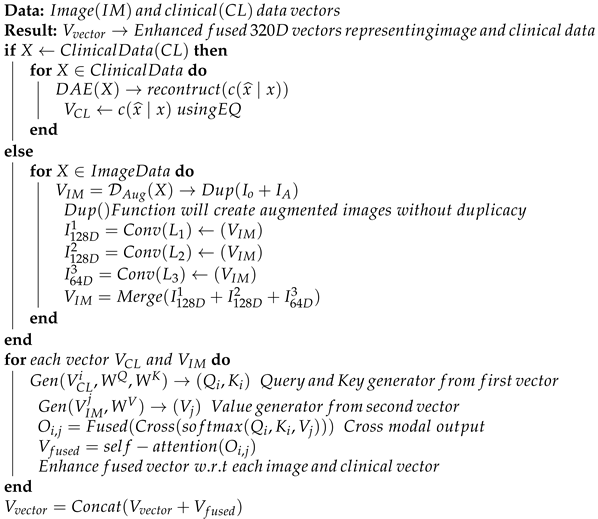
The multi-modal TB disease dataset includes clinical health records and chest X-ray images for 3256 patients. It was obtained from Government Medical College in Uttarakhand, India. The dataset is categorized among two classes labeled as ‘Tuberculosis Diagnosed (TB)’ or ‘Tuberculosis Not Diagnosed (NTB)’. The dataset was created for internal research purposes only and is not available for public use. The sample dataset is illustrated in Figure 1.
The dataset includes 3558 paired clinical records, each with a corresponding labeled chest X-ray image for the patient. For some of the patients, the procedure was performed few times that make the available paired clinical records slightly higher than the number of patients. The total number of TB class records were 1489 and the NTB class were 2069. The dataset consists of 2340 male and 916 female patients, with age ranges of 24–78 years and 35–68 years, respectively. The clinical health records consists of only most relevant features associated with the disease at the time of patient admission. The clinical features such as sputum test, body temperature, hemoglobin, blood pressure, smoking habits etc. are present in the dataset.
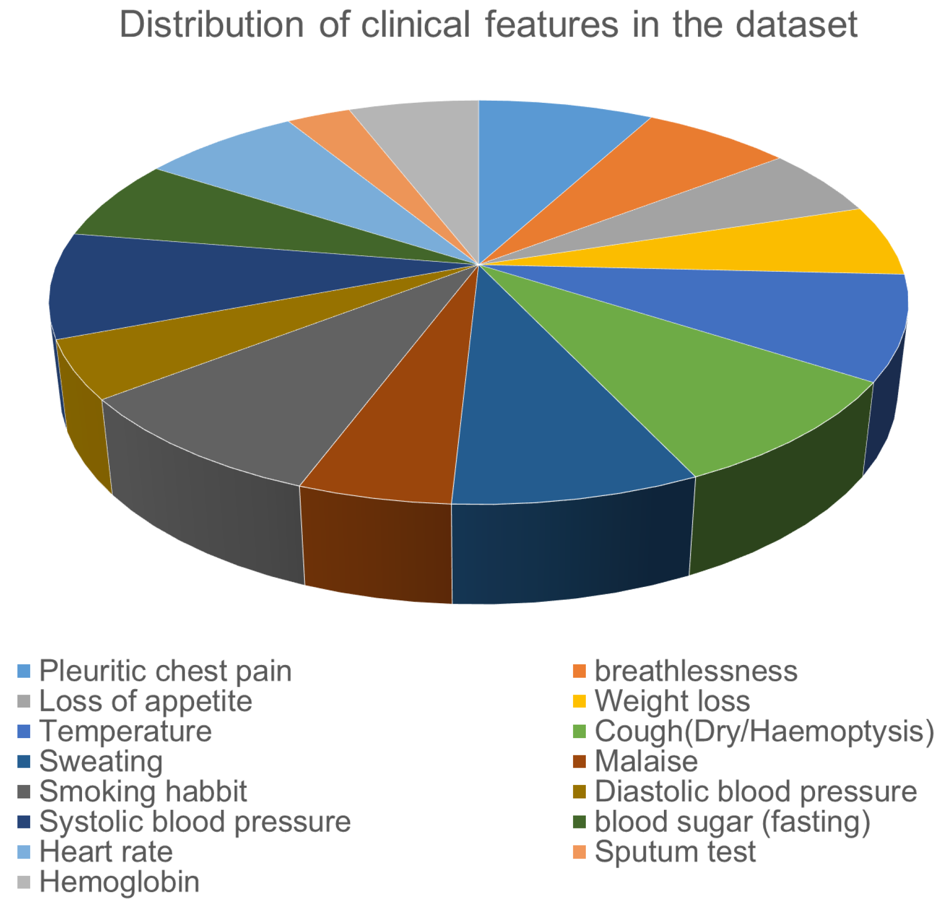
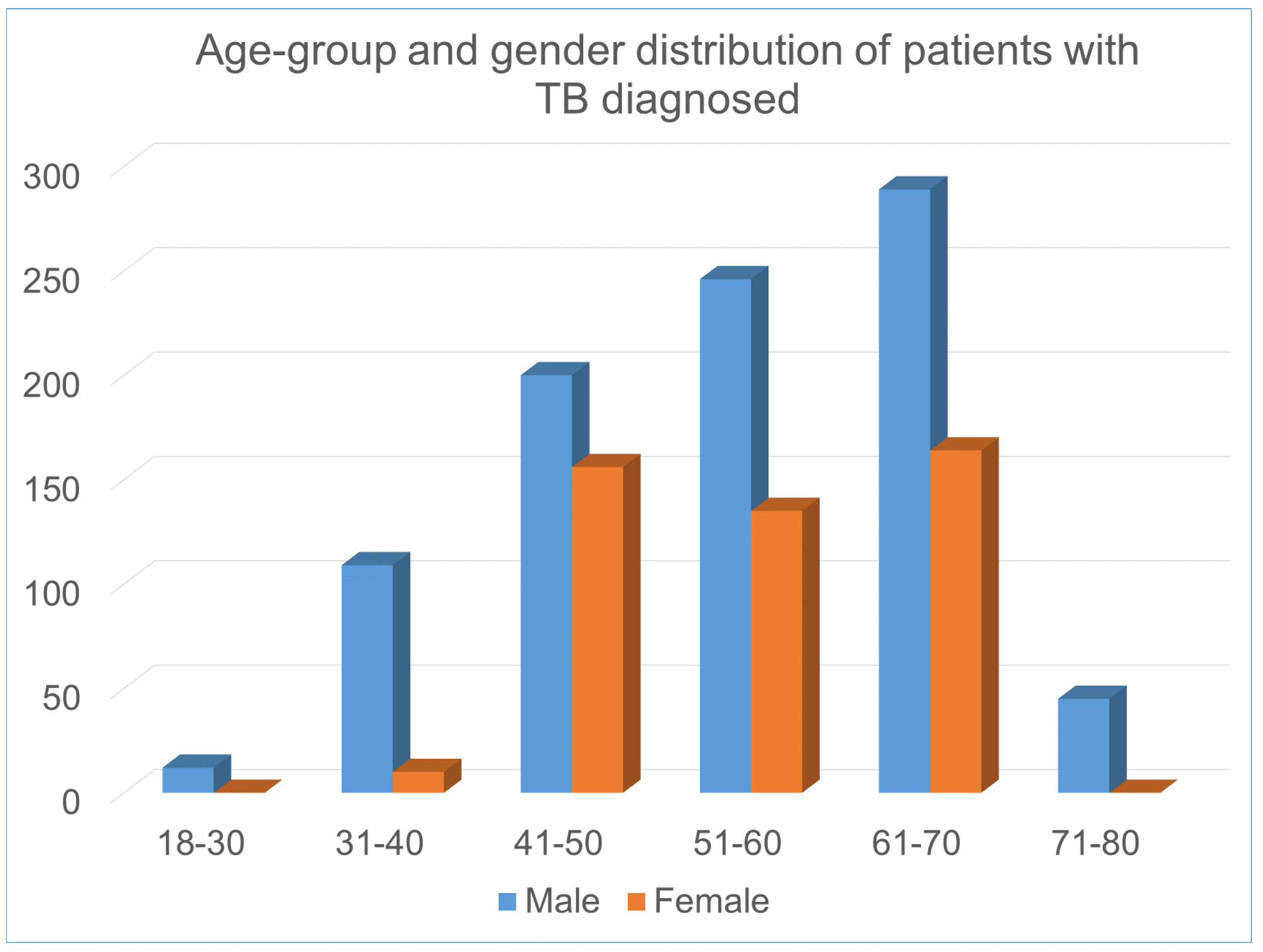
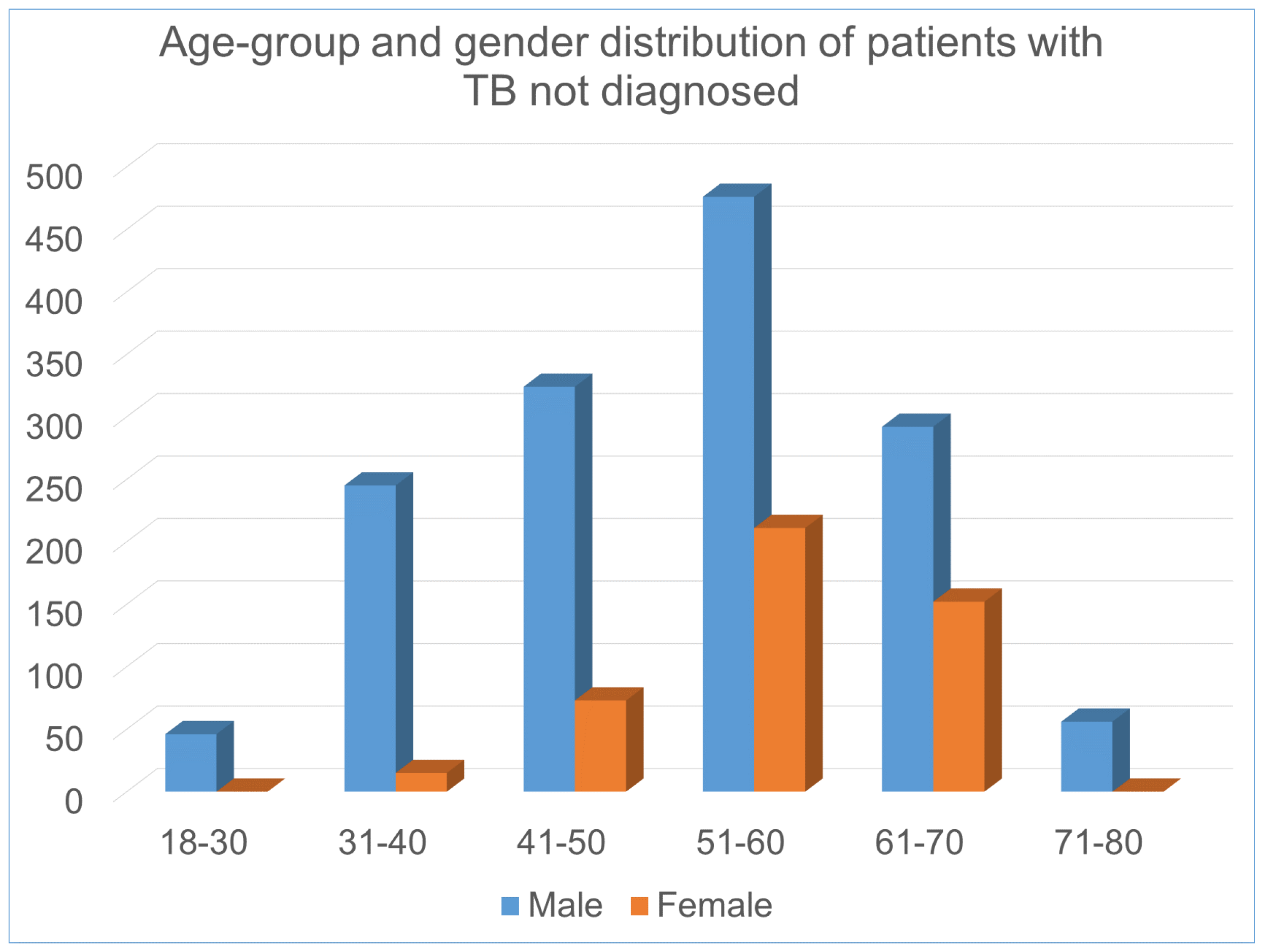
The complete set of clinical features, their types are shown in Table 1. Figure 2 shows the distribution of the patients with abnormal values in different clinical features in the dataset. In addition, Figure 3 and Figure 4 illustrates the age and gender wise distribution of patients diagnosed with TB and not diagnosed with TB respectively.
It is evident that in the dataset, majority of male TB patients falls within 31–70 age group, whereas female patients falls within 41–70 age group. The overall description of the dataset is presented in the table and figures are given below:

3. Proposed Methodology

3.1. Proposed Framework

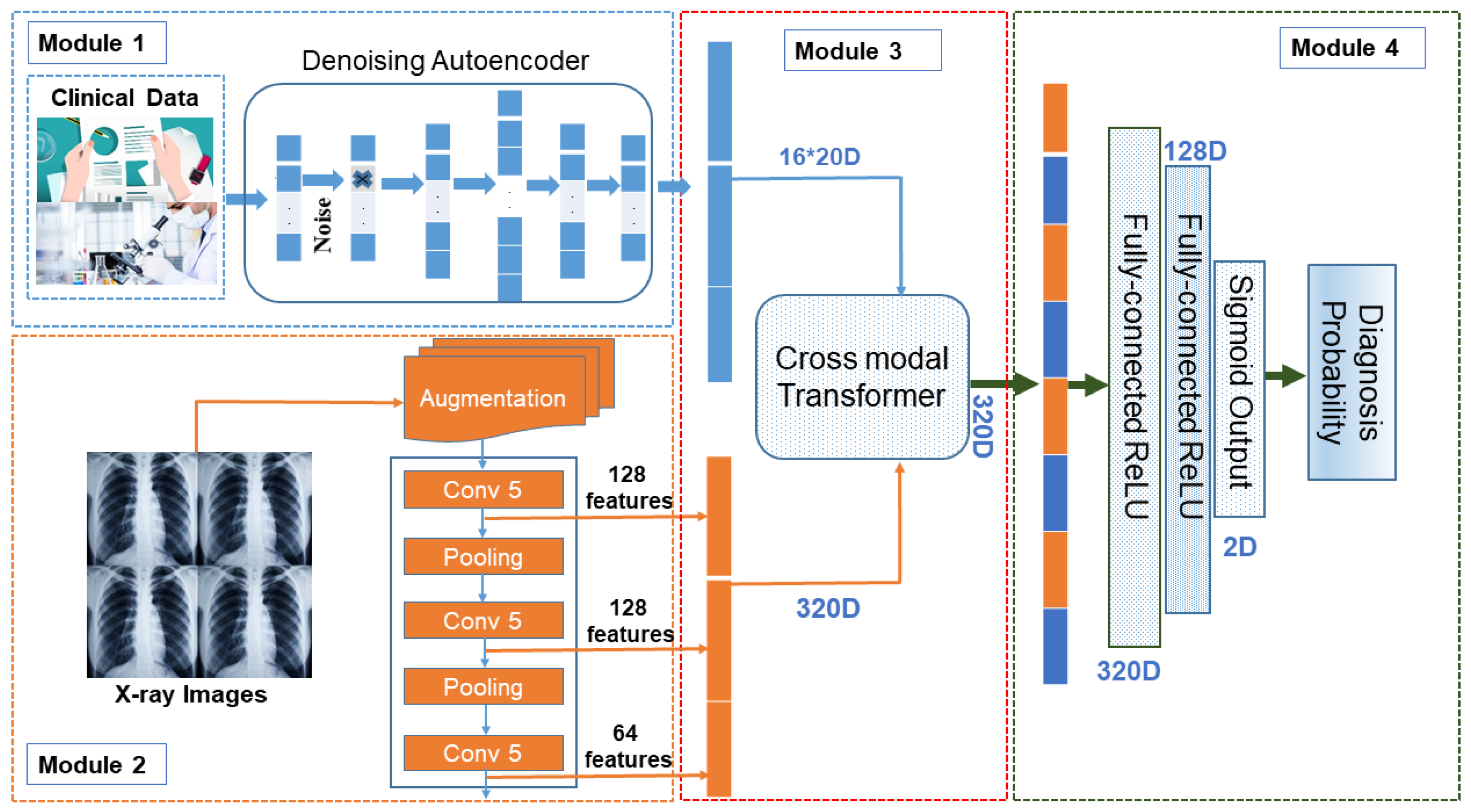
In the medical world, we broadly deal with two forms of data i.e., textual data (clinical symptoms, medical reports, test reports, etc.) and image data (X-ray). We propose a modal that can deal with both kinds of data to predict the probability of whether the patient is suffering from the disease or not. The overall working of the proposed modal is presented in Figure 5.
The proposed modal is divided into four basic modules. We define each module in detail as follows:

3.1.1. Module1: Clinical Data Processing ( M 1 )

An autoencoder is an artificial neural network used for learning unlabeled data coding efficiently. The autoencoder has two learning functions: a coding function, which converts the input data, and a decoding function, which reconstructs the input data from the coded representation. The purpose of the autoencoder is to learn an efficient representation for a set of data, usually for dimensionality reduction. An encoder can be defined as two sets one representing the space of decoded messages X and another representing the space of encoded messages Z where both X = R m and Z = R n are euclidean spaces. These are parameterized as
E ϕ : X Z
D θ : Z X w h e r e ϕ a n d θ a r e p a r a m e t e r s
For any x X we get z = E ϕ ( x ) and is called as latent variable as shown in Equation (1) and z Z we get x = D θ ( z ) and is called as decoded text or input as shown in Equation (2). Since, clinical healthcare data has relatively less features than X-ray imaging modality, In order to minimize the loss of information for each modality, it is necessary to increase the low dimensional modality rather than to reduce the high dimensional modality prior to data fusion. It ensures that each modality has sufficient information before fusion, which is a prerequisite for effective fusion. Due to lower features in clinical data autoencoder faces the issue of identity function i.e., null function hence, autoencoder doesn’t work well for our scheme. Therefore we propose using a Denoising Autoencoder (DAE) [16]. We use denoising autoencoder as a way to increase the data dimension to achieve the goal of improving the effectiveness of the data fusion and the robustness of the methods. Autoencoder is a kind of unsupervised machine learning model whose output data are a reconstruction of the input data, and it is often used for dimensionality reduction. However, there has been little use of autoencoders or their variants to increase the dimension of data. Denoising autoencoder shares the same structure as autoencoder, but the input data are noisy versions of the raw data. To force the encoder and decoder to learn more robust feature representation and prevent them from simply learning the identity function mapping, the autoencoder is trained to reconstruct the raw input data from its noisy versions. Because the features that we extracted from the structured data are 16 dimensions, there are 16 nodes in the input layer of the denoising autoencoder. After many experiments, the numbers of network nodes of the denoising autoencoder that we finally adopted are 16, 100, 216, 320, 216, 100 and 16. DAE is an autoencoder [17] that adds noise to the training data first and then provides noisy clinical data as input. Further, DAE is trained to predict the original, uncorrupted data point as the output. This happens by instructing the encoder and decoder to learn more robust features of the original dataset. The difference between the original and reconstructed data vector is treated as an error and is minimized during the training process. DAE is trained to reconstruct the clean point x from its corrupted version x ^ which is obtained through corruption process i.e., C ( x ^ x ) as shown in Equation (3). Further, the loss function is minimized using Equation (4).
c ( x ^ | x ) = N ( μ = x , = σ 2 I )
L = l o g P d e c o d e r ( x h = f ( x ^ )
where P d e c o d e r is a factorial distribution whose parameters are provided by a feed-forward network N.
DAE uses ( x x ^ ) as a training data point and estimates the reconstruct distribution P r e c o n s t r u c t ( x x ^ ) which is equivalent to P d e c o d e r ( x x ^ ) . The static gradient decent performed by DAE can be presented as
E x p ^ d a t a ( x ) E x ^ C ( x ^ x ) l o g P d e c o d e r ( x h = f ( x ^ ) )
where p ^ d a t a ( x ) is a training distribution.
The next step is to match the score of the modal with the data distribution at every data point x i.e., x l o g P ( x ) . DAE employee conditional Gaussian P ( x h ) for learning vector field g ( f ( x ) x ) which in turn estimates the score of the data distribution. While training DAE we have used squared error ( g ( f ( x ) x 2 ) for optimizing the model.
Finally, the module generates 16 × 20 D vector embeddings C d = { C T 1 , C T 2 , , C T n } representing original clinical data. These generated embeddings are fed as input to Module 3 discussed in Section 3.1.3. The working of module is shown in Figure 6.

3.1.2. Image Data Processing Module M 2

Parallel to module M 1 discussed in Section 3.1.1, the image data is provided as input to CNN using augmentation.
Insufficient data usually prevents training the modal and applying this under-trained modal to over-generalized new data causes issues like overfitting. Augmentation is a solution to such problems. Increasing samples with some random changes and producing realistic-looking data images help the model to get better trained. Augmentation assures that there is no duplicity of the image hence, the modal never sees the same image again. This makes the modal to be more generic and exposes different features of data. Final augmented data is presented as:
D A u g = { I o 1 , I o 2 , I o m . + . I A 1 , I A 2 I A n }
where m were original images, n are new augmented images and new dataset D A u g contain total m + n images. This new dataset D A u g is provided as input to the neural network (CNN). A basic CNN carries 5 layers Input, Convolution, Pooling, Dense, and Output. Input image is fed into convolution layer where filter f is slides over input image I which in-turn transforms image and maps features values according to Equation (6)
G [ x , y ] = ( I f ) [ x , y ] = j k f [ j , k ] I [ x j , y k ]
where x and y are resultant feature map matrix dimensions. CNN layer evaluate the intermediate value Z which is obtained as Z l = W l . A [ l 1 ] + b l where A is activation function A [ l ] = g [ l ] ( Z [ l ] ) . In our proposed model we used ReLU activation function f ( x ) = m a x ( 0 , x ) and use mean squared error (MSE) as a loss function i.e.,
L ( h ( x ) , x ) = 1 n i = 0 n ( h ( x ) i x i ) 2
This helps in gaining global minima and good training of the CNN.
In our proposed model we propose to have 3 sandwiched layers of CNN with pooling in between them. Layer one and two generates 128 feature maps and layer three generate a feature map of 64. Finally, they are combined to produce a feature embedding vector of size 320D i.e., I d = { I M 1 , I M 2 I M m } . Vectors of size 320D generated by each Module M 1 and M 2 are fed as input to the next component called a cross-modal transformer.

3.1.3. Cross-Modal Transformer M 3

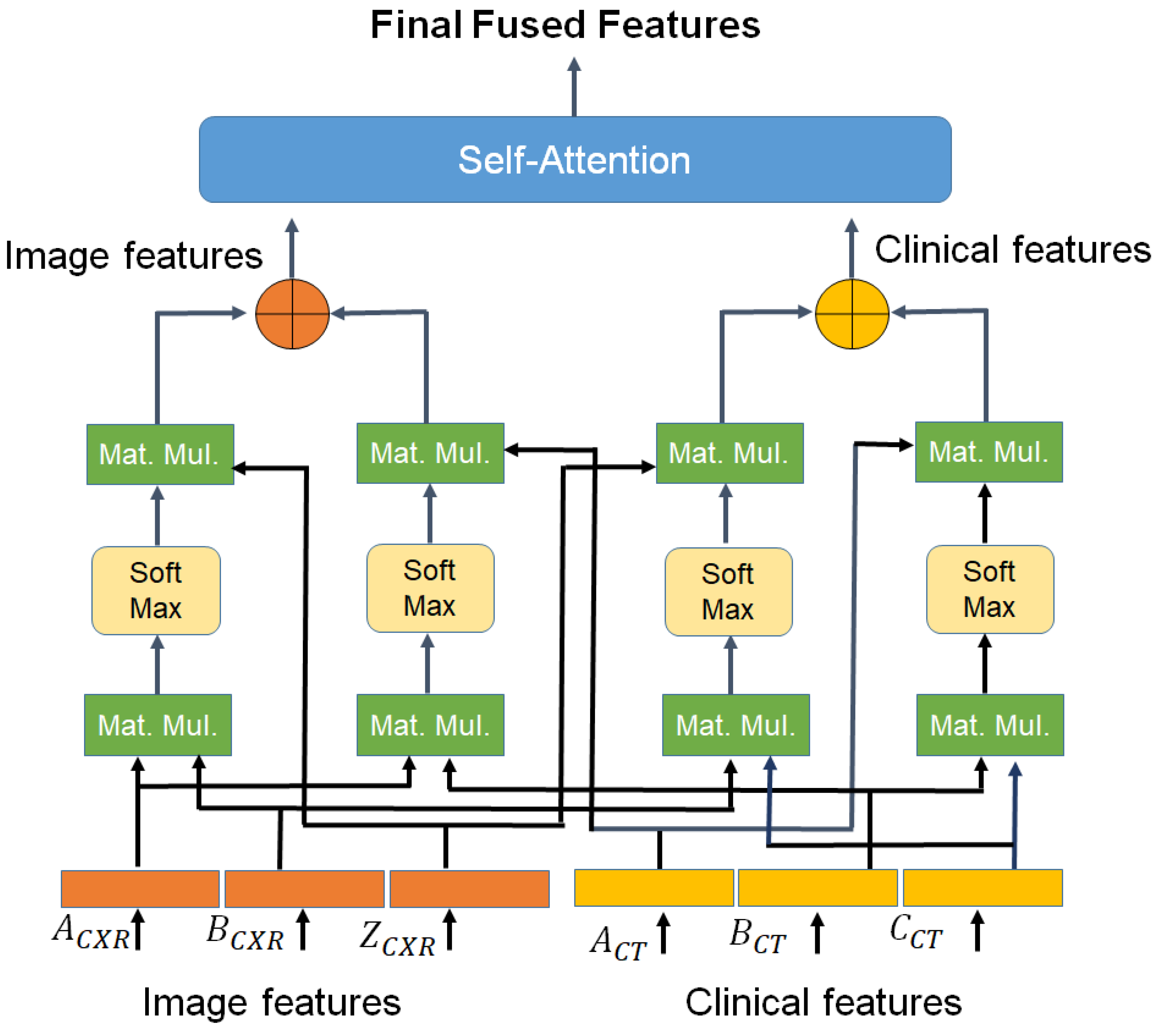
In this module, we proposed to use a two-head cross-modal with one head for image and a second head for clinical data. Once the cross-modal transformer layer is fed with 320D embedding generated in previously discussed modules, it transforms them into fused feature vectors as shown in Figure 7. A cross-modal transformer combines asymmetrically two separate embedding sequences of the same dimension. It uses query Q X i and value V Y i from one sequence, and key K Y j from the other where ( x , y ) [ C d , I d ] embedding sets.
Q X i = X i W Q ; K Y j = Y j W k : V Y j = V i W V
where W Q , W K , and W V are learn-able weights. Further, the cross-modal used to evaluate attention by using the Softmax function presented in Equation (8)
C r o s s ( Q X i , K Y j , V Y j ) = S o f t m a x Q X i K Y j T d k V j
The resulting cross-attention modal is passed through a linear layer W o project and the output obtained is a fused feature vector of 320D.
o u t p u t = C r o s s ( Q X i , K Y j , V Y j ) W o
The output is further passed through a self-attention layer. self-attention mechanism is employed for enhancing the information content of the produced output. Unlike cross, this layer generates Query and key from one feature vector i.e., Q i = W Q X i and K i = W K X i and value i.e., V j = W V Y j from another feature vector. Further, un-normalized attention weight is evaluated to determine the weight of input elements w i = Q i T K j and score as in Equation (9)
α j , i = S o f t m a x w j i d K
Finally, the self-attention layer computes context vector Z 2
Z = i T α j i V j
In Equation (10), the variable T, represents the length of input feature vector. Z 2 is the attention-weighted version of our original query input X 2 . This layer enables the model to weigh the importance of different elements in an input sequence and dynamically adjust their influence on the output. This resultant enhanced fused feature vector 320D is provided as input to the classification module discussed next Section 3.1.4.
The entire processing phases discussed so far can be presented in Algorithm 1. The algorithm takes both images and clinical data vectors as input and processes them to generate an enhanced fused vector V f u s e d possessing an enriched format to be given as input to the classification layer. This will help in improving overall classification accuracy.
Algorithm 1 Psuedocode for generating enhanced feature vectors for improved classification
Bdcc 08 00125 i001

3.1.4. Disease Probability Prediction Module M 4

The prediction module takes this fused feature vector of image and clinical data as input, processes it, and produces the final prediction probability of whether the patient suffering from the disease or not. The module carries multiple fully connected ReLU layers of 320D and 128D. Further, the final layer is a sigmoid 2D layer which final classifies the patient features and produces the respective probability. We have employed a fully connected layer in the proposed model. Initially, A linear transformation with a weight matrix followed by a nonlinear activation function is applied to the feature vector by each neuron as shown in Equations (11) and (12).
Y j k ( X ) = f i = 1 n , m W j k X i + W j 0
f = F ( x ) = m a x ( 0 , x ) = R e L U
This ensures that every input of the feature vector influences every output of the output feature vector, creating all possible connections layer-to-layer. The first fully connected ReLU layer converges 320D vector into 128D features. This helps in gaining a lower dimension vector but retaining the similar statistics as the 360D input vector. 128D vector is further processed to generate a 2D feature vector. The convergence helps in mapping the larger feature set to the more knowledgeable small feature set to make prediction more accurate. The final layer uses the Sigmoid activation function as shown in Equation (13).
ϕ ( Z ) = 1 1 + e Z
Sigmoid function is used primarily because it exists between ( 0 to 1 ) and probability i.e., P ( 0 to 1 ) . For this reason, it is used in particular for models in which we need to predict the probability as an output. This multiple layer makes the model more robust and accurate for disease probability prediction. In addition, we used the MSE (Mean squared error) function with L 2 regularization penalty term is used as the control function as shown in Equation (8) as follows:
M i n i m i z e L o s s L = 1 N a = 1 N ( y i y i ^ ) 2 + λ b = 1 M ω j 2
where ω j is the model parameter, and λ is the penalty coefficient term. The pseudocode for the discussed classification phase is presented in Algorithm 2.
Algorithm 2 Pseudocode for classification using Multi-layer Dense Neural Network
Bdcc 08 00125 i002
The models work well with both data categories i.e., clinical and image data as well as manage to provide better accuracy even if we have fewer data available. This helps in improving our medical facilities and early-stage disease detection. The performance of the proposed scheme is detailed in Section 4.

3.2. Model’s Classification Performance Measure

An important factor in classification is the ability of the classifier to accurately predict outcomes for unobserved instances. The following classification metrics are used to evaluate the effectiveness of the developed approach and to compare it to existing methods:
  • TP, TN, FP and FN:
    • TP (True positive): In our approach true positive is taken as the number patients with tuberculosis in original dataset and are correctly identified.
    • TN: (True Negative): It shows the total number of patients who are not suffering from tuberculosis and being correctly identified.
    • FP (False Positive): This term reflects the total number patients who are not suffering from tuberculosis but model classified them as one.
    • FN (False Negative): This term Presents the number of patients who were suffering from tuberculosis but were not identified and were marked as healthy.
  • Prediction Accuracy: Accuracy is a crucial parameter in distinguishing between patient and healthy cases. To achieve this, we evaluate the proportion of true positive cases and the proportion of true negative cases in each case, as shown in the following Equation (15):
    A c c u r a c y = T P + T N T P + T N + F P + F N
    where T P and T N present the sample patients which have been classified as positive and negative correctly respectively.
  • True Positive Rate (TPR) and False Positive Rate (FPR): Also referred to as the sensitivity of a classifier, TPR measures the proportion of correctly identified positive events. FPR, on the other hand, is the probability of false rejection of the null hypothesis. It divides the number of negative events falsely classified as positive by the total number of true negative events. TPR can be calculated as Equation (16), and FPR can be calculated as Equation (17).
    T P R = T P T P + F N
    F P R = F P F P + T N
  • Precision: Precision is a metric that is widely used to evaluate the performance of a classification algorithm. It measures the exactness of the algorithm’s results and can be defined as a measure of exactness. Mathematically, precision can be expressed as shown in the Equation (18).
    P r e c i s i o n = T P T P + F P
    where F P is the number of patients who have been classified as positive but are negative.
  • Specificity: The classifier’s specificity refers to its ability to accurately predict negative cases within a given dataset. This can be calculated as a metric of performance as given in Equation (19):
    S p e c i f i c i t y = 1 F P F P + T N
  • F-measure (F-score): The F-measure, also known as the F-score, is a metric used to evaluate the accuracy of a classifier test [18]. It is calculated by taking into account both precision and recall, and is defined as the harmonic mean of these two values. The F-score ranges from 0 to 1, with 1 being the ideal value and 0 being the worst. F-score can be calculated as given in Equation (20).
    F - M e a s u r e = 2 P r e c i s i o n R e c a l l P r e c i s i o n + R e c a l l
  • Matthews correlation coefficient (MCC): The Matthews correlation coefficient (MCC) is a balanced metric used to measure the quality of binary classification when the predicted variable has only two values [19]. In our scenario, the target attribute has two class values: ‘TB’ and ‘NTB’. The MCC is particularly useful when dealing with imbalanced classes. Its value ranges between + 1 to 1 . A value of + 1 is considered as a perfect prediction, 0 for average prediction and 1 for no prediction. MCC can be calculated as Equation (21).
    M C C = ( T P × T N ) ( F P × F N ) ( T P + F P ) ( T P + F N ) ( T N + F P ) + ( T N + F N )
  • Receiver operating characteristic (ROC) curve: The ROC (Receiver Operating Characteristic) is a crucial measure for evaluating classifier accuracy [20]. Originally developed in signal detection theory, it shows the connection between hit and false alarm rates while taking into account channel noise. Nowadays, ROC is widely used in the field of machine learning as a valuable tool for visualizing classifier performance. The ROC curve illustrates the correlation between True Positive Rate (TPR) and False Positive Rate (FPR). To evaluate the performance of the classifier, we calculate the AUC (area under the ROC curve). An AUC value close to 1 indicates excellent performance, while a value less than 0.5 indicates poor performance.

4. Experiments and Results

This section discusses the experiments performed and results obtained using the proposed framework on the multimodal TB dataset.

4.1. Experimental Setup

The experiments were conducted on a Fujitsu 64-bit workstation with 64 GB of RAM, 48 cores, and 2 TB of storage. The method was trained and evaluated on multimodal data with a 10-fold cross-validation split. The dataset is divided into three parts: training, validation, and test data, in a 6:2:2 ratio respectively. The validation dataset is used to fine-tune and optimize hyperparameters, such as the penalty coefficient. The model was trained until 200 epochs using Adam as the optimizer. The batch size parameter is set to 64, and the initial learning rate is 0.001, subsequently decreasing by 0.5 every 40 epochs. Additionally, the learning rate is reduced by 0.5 every 40 epochs. The batch size parameter is set to 64, and the initial learning rate is 0.001, subsequently decreasing by 0.5 every 40 epochs. The batch size parameter is set to 64, and the initial learning rate is 0.001, subsequently decreasing by 0.5 every 40 epochs. The algorithm reached the convergence in 150 epochs and after that there was no improvement in the accuracy.

4.2. Multimodal Data Processing and Fusion

The multimodal TB dataset is provided with labeled X-ray images and clinical healthcare data. In order to perform, multimodal analysis, both X-ray and clinical healthcare modalities were processed differently. The 16 clinical health features were expanded to 320 features using a denoising autoencoder, as explained in module M1 of the proposed framework. For the imaging modality, the X-ray images were first enhanced by removing noise and resized to a resolution of 224 × 224. Augmentations were performed using rotation, shearing, zooming, shift and flip techniques. Additionally, the image features were extracted via module M2 of the proposed framework. The cross-modal attention block was used to fuse the extracted features from imaging and clinical modalities for the TB diagnosis module.

4.3. Ablation Study and Performance Comparison with Existing Models

We conducted an ablation study to determine the best classification architecture for the final module of the proposed framework. Four three-layer neural network (NN) architectures, [ 320 × 128 × 2 ] , [ 320 × 64 × 2 ] , [ 320 × 32 × 2 ] , [ 320 × 16 × 2 ] , and one NN architecture without hidden layer [ 320 × 2 ] for TB classification. The Table 2 illustrates the performance of different NN architectures on complete multimodal dataset. It was observed in ablation study that the 3-layer NN architecture with one hidden layer with [ 320 × 128 × 2 ] dimension achieved the higher accuracy and minimum loss on full dataset.
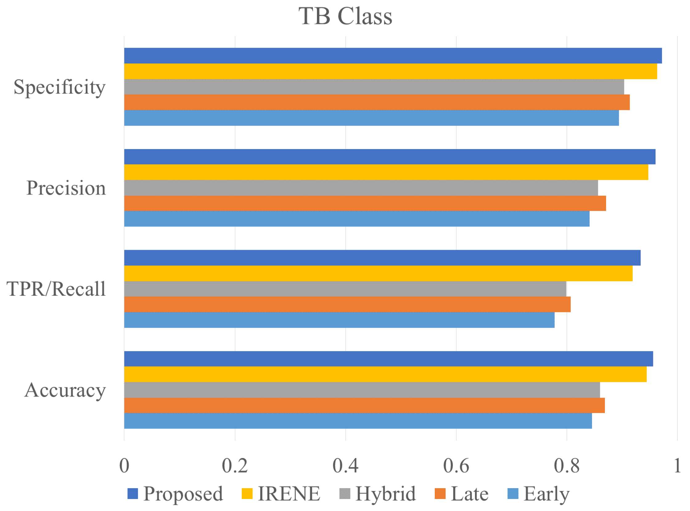
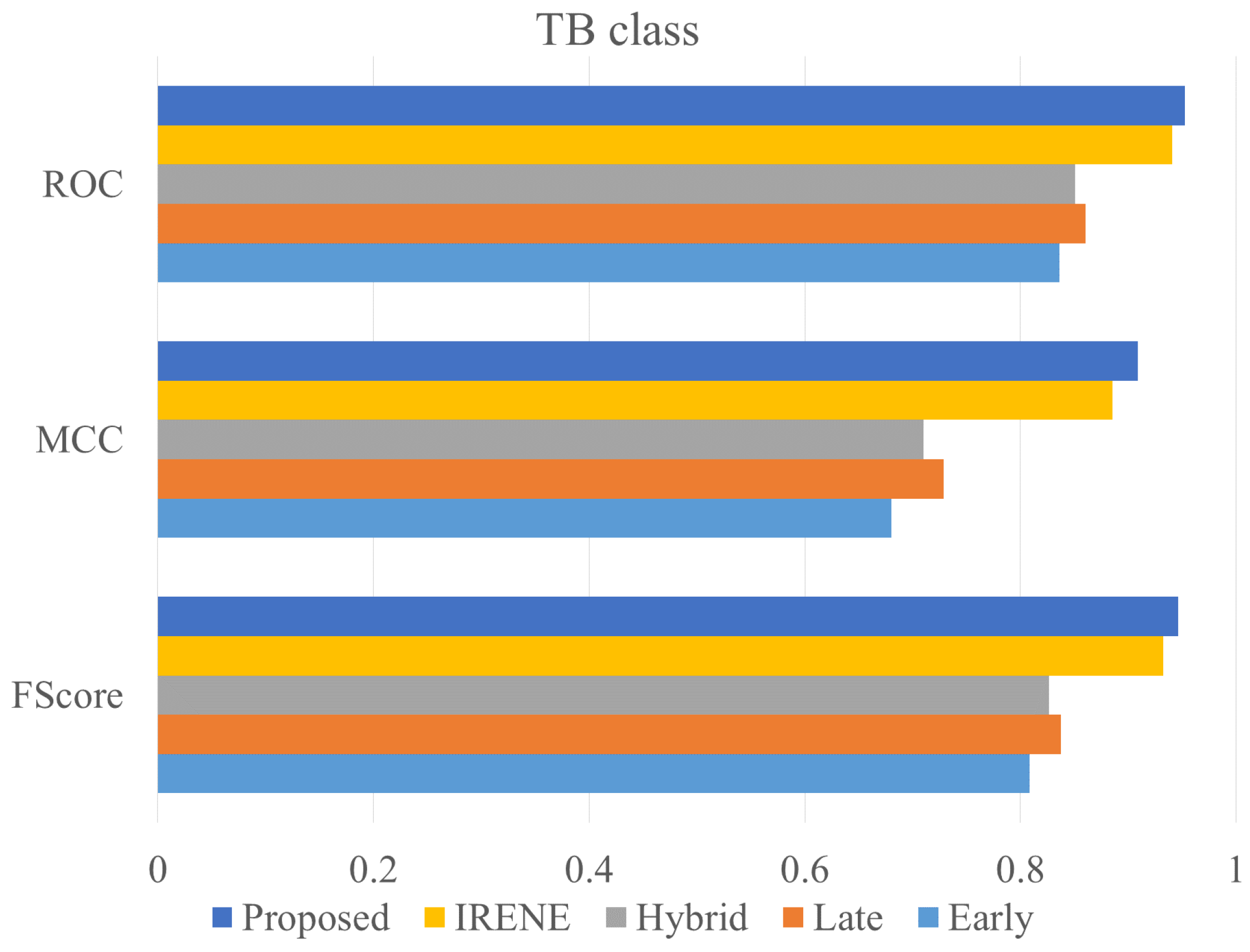
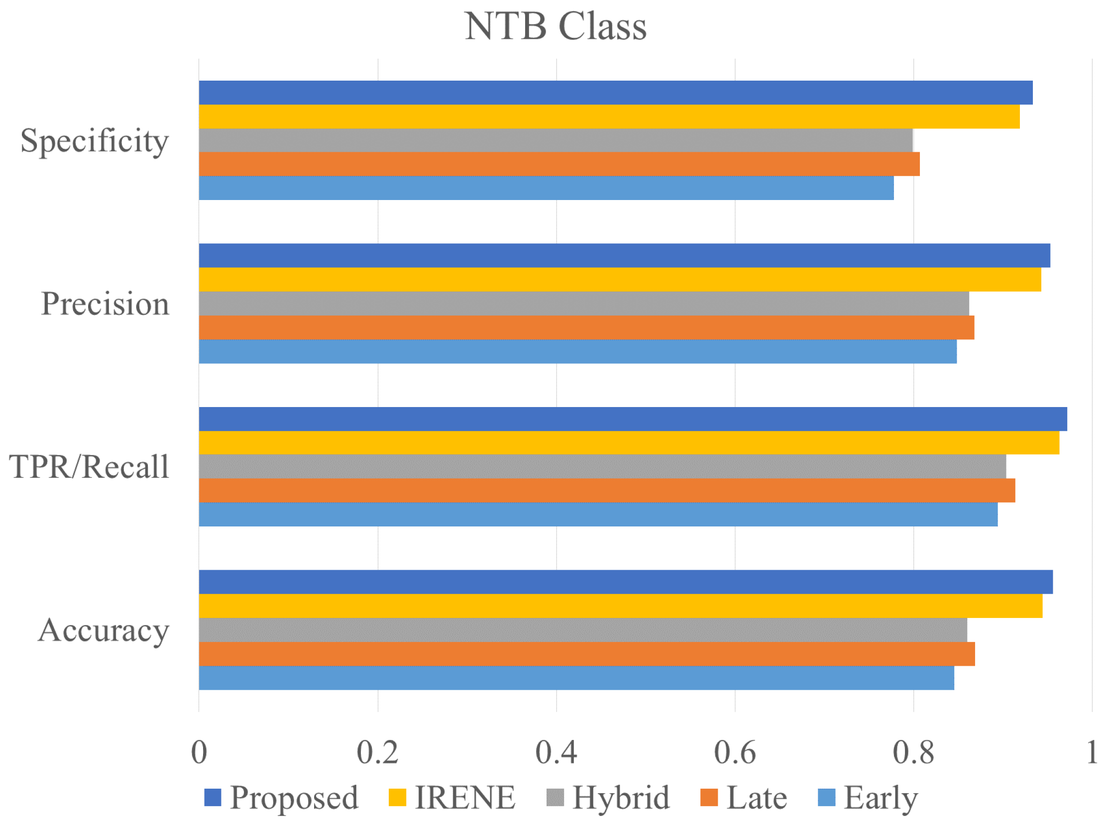
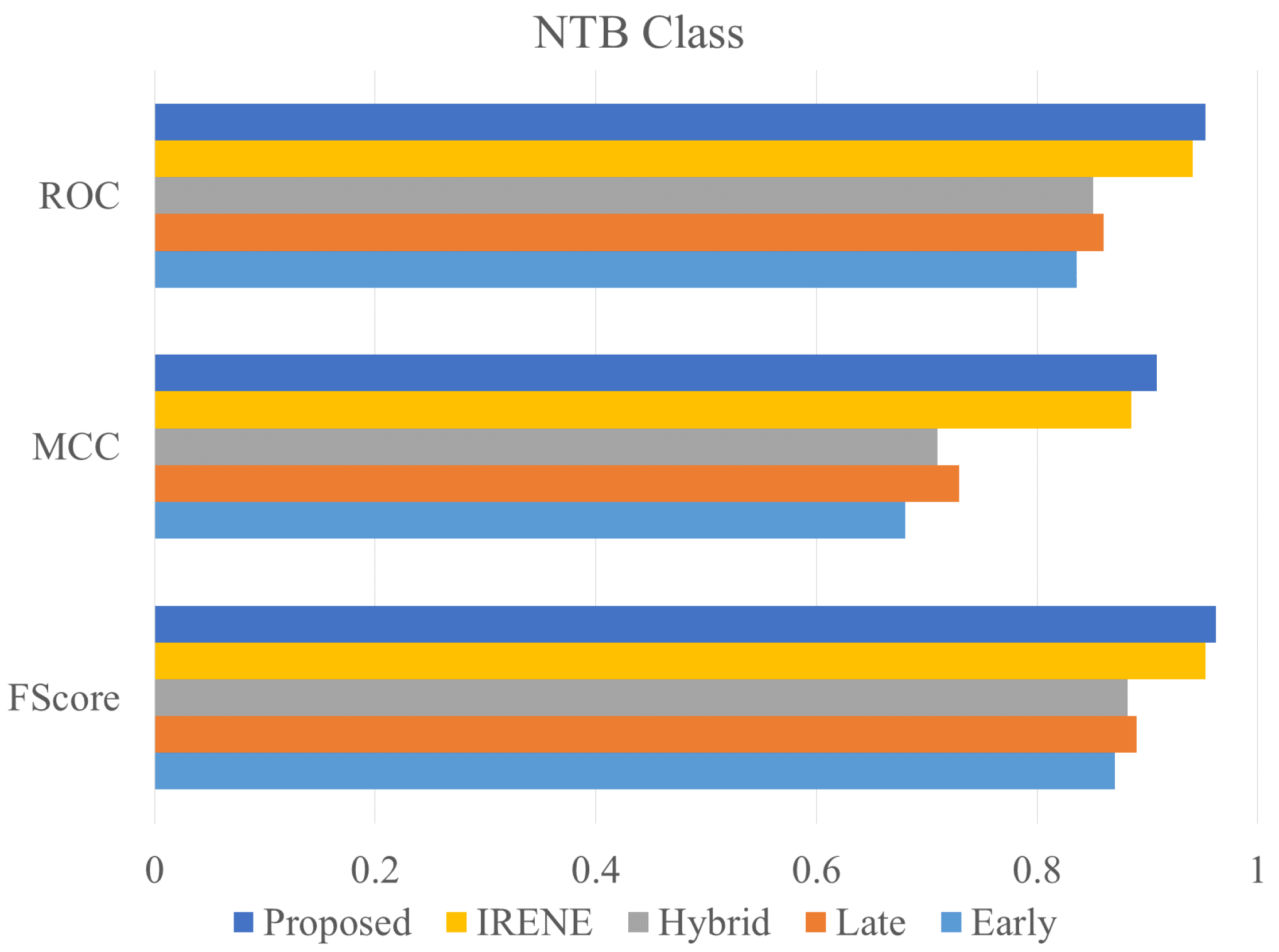
To evaluate the performance of the proposed model, different classification metrics i.e., accuracy, recall, precision, Fscore, MCC, ROC are used. In addition, existing fusion models such as early fusion, late fusion, hybrid fusion models were also developed and evaluated on the dataset. Furthermore, we also compared the performance of our model with IRENE, a transformer enabled unified representation approach proposed by Zhou et al. [15] on our dataset. The results in the Table 3 shows that our proposed model outperforms the traditional fusion models in all the parameters. The Early Fusion model has the lowest performance of all models. Also, early fusion is not recommended for heterogeneous modality fusion. The late and hybrid fusion models achieved slightly better performance than the early fusion models. Furthermore, the performance of IRENE was remarkable. As the authors [15] claimed, the unified representation certainly helps in increasing the classification performance. The accuracy with IRENE got an improvement of about 9% on our TB dataset. However, our model outperformed IRENE with a slightly improved margin on our dataset. The confusion matrix is given in Figure 8. Figure 9, Figure 10, Figure 11 and Figure 12 illustrates the performance of all models tested on TB dataset for both TB and NTB class on different evaluation parameters. The results indicate that the proposed model achieved the lowest false positive rate (FPR) compared to all other models. Additionally, the proposed model has the highest receiver operating characteristic (ROC) score, Matthews correlation coefficient (MCC), and F-score. These parameters demonstrate that utilizing a cross-modal transformer approach with the appropriate neural network architecture can lead to improved performance in tuberculosis diagnosis. The ROC comparison is shown in Figure 13.

5. Conclusions

The paper proposes a deep learning approach that utilizes a cross-model transformer block to diagnose TB disease using a new multimodal TB dataset. The dataset comprises of two modalities: clinical healthcare data and medical imaging X-rays. The proposed framework enhances the clinical data features to match the imaging modality features using a denoising autoencoder module. The imaging modality features are extracted using a CNN architecture. A cross-modal attention block is used to combine features and provide a unified set of features for the final TB diagnosis module. An ablation study was conducted to determine the best neural network architecture for classification. The results showed that the proposed transformer-enabled deep learning approach outperformed other traditional fusion approaches on various classification metrics. The study’s limitation is the availability of less number of clinical features in the multimodal dataset. Additional clinical features can be included in the dataset based on the recommendation of the pulmonologist, which will certainly enhance the reliabiity of disease diagnosis model. Moreover, advanced approaches for multimodal data fusion can be developed for medical diagnosis. Another limitation is the number of available medical records for developing the deep learning based model for disease diagnosis. There is big requirements to create a multimodal dataset for various diseases so that an effective and reliable AI based model can be developed. The medical research centres must take efforts in this direction.

Author Contributions

Conceptualization, S.K. and S.S.; methodology, S.K. and S.S.; software, S.K. and S.S.; validation, S.K. and S.S.; formal analysis, S.K. and S.S.; investigation, S.K. and S.S.; resources, S.K. and S.S.; data curation, S.K. and S.S.; writing—original draft preparation, S.K. and S.S.; writing—review and editing, S.K. and S.S.; visualization, S.K. and S.S.; supervision, S.K.; funding acquisition, S.K. All authors have read and agreed to the published version of the manuscript.

Funding

This study is supported by the Russian Science Foundation regional grant no. 23-21-10009.

Data Availability Statement

The data is not publicly available to use. However, with the permission of Government of Uttarakhand, the data can be requested.

Acknowledgments

Authors are thankful to the Government of Uttarakhand, India to provide support in achieving the data for research purpose. We also thankful to the medical students and senior practitioners to provide assistance in preparing the multimodal dataset for tuberculosis patients.

Conflicts of Interest

The author declares no competing interest to delcare regarding the publication of this article.

References

  1. Tuberculosis. Available online: https://www.who.int/news-room/fact-sheets/detail/tuberculosis (accessed on 10 December 2023).
  2. Esteva, A.; Chou, K.; Yeung, S.; Naik, N.; Madani, A.; Mottaghi, A.; Liu, Y.; Topol, E.; Dean, J.; Socher, R. Deep learning-enabled medical computer vision. NPJ Digit. Med. 2021, 4, 5. [Google Scholar] [CrossRef] [PubMed]
  3. Aiadi, O.; Khaldi, B. A fast lightweight network for the discrimination of COVID-19 and pulmonary diseases. Biomed. Signal Process. Control 2022, 78, 103925. [Google Scholar] [CrossRef] [PubMed]
  4. Guan, B.; Yao, J.; Zhang, G. An enhanced vision transformer with scale-aware and spatial-aware attention for thighbone fracture detection. In Neural Computing and Applications; Springer: Berlin/Heidelberg, Germany, 2024; pp. 1–14. [Google Scholar]
  5. Boulahia, S.Y.; Amamra, A.; Madi, M.R.; Daikh, S. Early, intermediate and late fusion strategies for robust deep learning-based multimodal action recognition. Mach. Vis. Appl. 2021, 32, 121. [Google Scholar] [CrossRef]
  6. Pandeya, Y.R.; Lee, J. Deep learning-based late fusion of multimodal information for emotion classification of music video. Multimed. Tools Appl. 2021, 80, 2887–2905. [Google Scholar] [CrossRef]
  7. Xu, T.; Zhang, H.; Huang, X.; Zhang, S.; Metaxas, D.N. Multimodal deep learning for cervical dysplasia diagnosis. In Proceedings of the Medical Image Computing and Computer-Assisted Intervention–MICCAI 2016: 19th International Conference, Athens, Greece, 17–21 October 2016; Proceedings, Part II 19. Springer: Berlin/Heidelberg, Germany, 2016; pp. 115–123. [Google Scholar]
  8. Schulz, S.; Woerl, A.C.; Jungmann, F.; Glasner, C.; Stenzel, P.; Strobl, S.; Fernandez, A.; Wagner, D.C.; Haferkamp, A.; Mildenberger, P.; et al. Multimodal deep learning for prognosis prediction in renal cancer. Front. Oncol. 2021, 11, 788740. [Google Scholar] [CrossRef] [PubMed]
  9. Vale-Silva, L.A.; Rohr, K. Long-term cancer survival prediction using multimodal deep learning. Sci. Rep. 2021, 11, 13505. [Google Scholar] [CrossRef] [PubMed]
  10. Joo, S.; Ko, E.S.; Kwon, S.; Jeon, E.; Jung, H.; Kim, J.Y.; Chung, M.J.; Im, Y.H. Multimodal deep learning models for the prediction of pathologic response to neoadjuvant chemotherapy in breast cancer. Sci. Rep. 2021, 11, 18800. [Google Scholar] [CrossRef] [PubMed]
  11. Steyaert, S.; Pizurica, M.; Nagaraj, D.; Khandelwal, P.; Hernandez-Boussard, T.; Gentles, A.J.; Gevaert, O. Multimodal data fusion for cancer biomarker discovery with deep learning. Nat. Mach. Intell. 2023, 5, 351–362. [Google Scholar] [CrossRef] [PubMed]
  12. Ivanova, O.N.; Melekhin, A.V.; Ivanova, E.V.; Kumar, S.; Zymbler, M.L. Intermediate fusion approach for pneumonia classification on imbalanced multimodal data. Bull. South Ural. State Univ. Ser. Comput. Math. Softw. Eng. 2023, 12, 19–30. [Google Scholar]
  13. Kumar, S.; Ivanova, O.; Melyokhin, A.; Tiwari, P. Deep-learning-enabled multimodal data fusion for lung disease classification. Inform. Med. Unlocked 2023, 42, 101367. [Google Scholar] [CrossRef]
  14. Lu, Z.H.; Yang, M.; Pan, C.H.; Zheng, P.Y.; Zhang, S.X. Multi-modal deep learning based on multi-dimensional and multi-level temporal data can enhance the prognostic prediction for multi-drug resistant pulmonary tuberculosis patients. Sci. One Health 2022, 1, 100004. [Google Scholar] [CrossRef] [PubMed]
  15. Zhou, H.Y.; Yu, Y.; Wang, C.; Zhang, S.; Gao, Y.; Pan, J.; Shao, J.; Lu, G.; Zhang, K.; Li, W. A transformer-based representation-learning model with unified processing of multimodal input for clinical diagnostics. Nat. Biomed. Eng. 2023, 7, 743–755. [Google Scholar] [CrossRef] [PubMed]
  16. Vincent, P.; Larochelle, H.; Bengio, Y.; Manzagol, P.A. Extracting and composing robust features with denoising autoencoders. In Proceedings of the 25th International Conference on Machine Learning, Helsinki, Finland, 5–9 July 2008; pp. 1096–1103. [Google Scholar]
  17. Bengio, Y. Learning deep architectures for AI. Found. Trends Mach. Learn. 2009, 2, 1–127. [Google Scholar] [CrossRef]
  18. Powers, D.M. Evaluation: From precision, recall and F-measure to ROC, informedness, markedness and correlation. arXiv 2020, arXiv:2010.16061. [Google Scholar]
  19. Matthews, B.W. Comparison of the predicted and observed secondary structure of T4 phage lysozyme. Biochim. Biophys. Acta (BBA)-Protein Struct. 1975, 405, 442–451. [Google Scholar] [CrossRef]
  20. Fawcett, T. An introduction to ROC analysis. Pattern Recognit. Lett. 2006, 27, 861–874. [Google Scholar] [CrossRef]
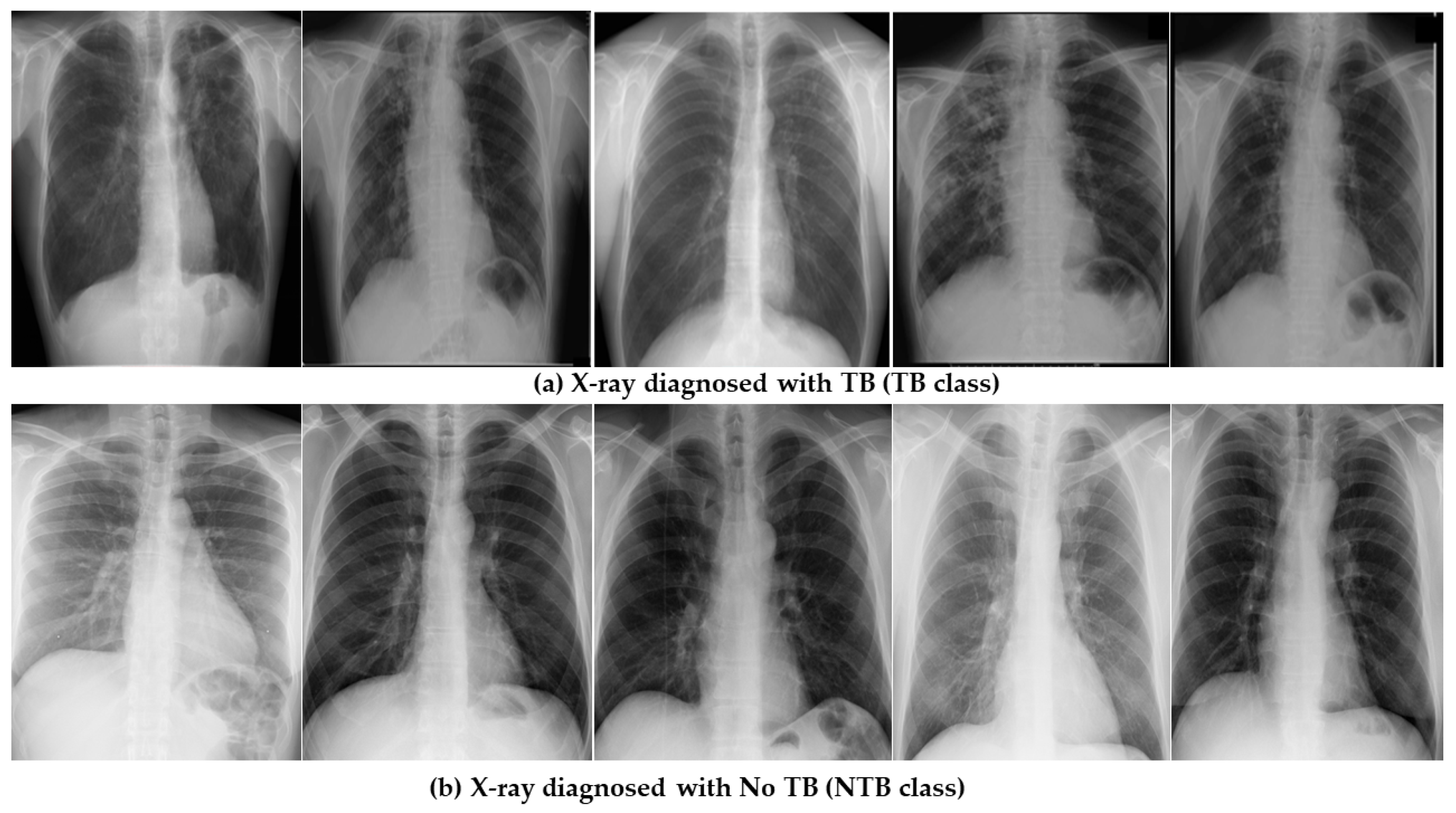
Figure 1. Sample dataset illustrating healthy and infected X-ray images.
Bdcc 08 00125 g001
Figure 2. Feature distribution in Clinical Data (abnormal values only).
Bdcc 08 00125 g002
Figure 3. Age and gender wise distribution of patients diagnosed with TB.
Bdcc 08 00125 g003
Figure 4. Age and gender wise distribution of patients not diagnosed with TB.
Bdcc 08 00125 g004
Figure 5. Proposed Framework where multi-modal data carrying text and image dataset are merged to generate 320D features using cross modal transformer. These are further transferred to dense connected layers for producing near probable classification.
Bdcc 08 00125 g005
Figure 6. Clinical feature processing using denoising autoencoder.
Bdcc 08 00125 g006
Figure 7. Cross model transformer block.
Bdcc 08 00125 g007
Figure 8. Confusion Matrix of proposed and other models compared.
Bdcc 08 00125 g008
Figure 9. Accuracy, precision, specificity and recall comparison of different models on TB class.
Bdcc 08 00125 g009
Figure 10. ROC, MCC, Fscore comparison of different models on TB class.
Bdcc 08 00125 g010
Figure 11. Accuracy, precision, specificity and recall comparison of different models on NTB class.
Bdcc 08 00125 g011
Figure 12. ROC, MCC, Fscore comparison of different models on NTB class.
Bdcc 08 00125 g012
Figure 13. ROC curve for different models used in the study.
Bdcc 08 00125 g013
Table 1. Overview of Clinical Features.
Clinical FeatureValue TypeValues
TemperatureContinuous97.1–103.3 °F
Diastolic blood pressureContinuous50–103 mm/Hg
Systolic blood pressureContinuous100–178 mm/Hg
blood sugar (fasting)Continuous80–170 mg/dL
Heart rateContinuous70–128 bpm
Patient’s HeightContinuous137–181 cm
HemoglobinContinuous6.0–19.3 g/dL
Body weightContinuous35–118 kg
Pleuritic chest painCategoricalY/N
Sputum TestCategoricalP/N
breathlessnessCategoricalY/N
Loss of appetiteCategoricalY/N
Weight lossCategoricalY/N
Cough (Dry/Haemoptysis)CategoricalD/H
MalaiseCategoricalY/N
Smoking habitCategoricalY/N
Table 2. Performance of different NN architectures for TB classification.
NN ArchitectureAccuracyLoss
[ 320 × 128 × 2 ] 95.590.0768
[ 320 × 64 × 2 ] 94.90.0985
[ 320 × 32 × 2 ] 94.60.1005
[ 320 × 16 × 2 ] 93.950.1039
[ 320 × 2 ] 90.860.1186
Table 3. Performance comparison of different fusion models on multimodal TB dataset.
ModelAccuracyTPR/RecallFPRSpecificityPrecisionF-MeasureMCCROCClass
Early Fusion0.84540.77770.10580.894140.84090.80800.68040.8359TB
0.84540.89410.22220.77770.84820.87050.68040.8359NTB
Late Fusion0.86870.80650.08650.91340.87020.83720.72900.8600TB
0.86870.91340.19340.80650.86770.89000.7290.8600NTB
Hybrid Fusion0.85940.79850.09660.90330.85600.82620.70970.8509TB
0.85940.90330.20140.79850.86160.88200.70970.8509NTB
IRENE [15]0.94430.91870.03720.96270.94670.93250.88540.9407TB
0.94430.96270.08120.91870.94270.95260.88540.9407NTB
Proposed Model0.95590.93280.02800.97190.95990.94610.90860.9524TB
0.95590.97190.06710.93280.95260.96220.90860.952403983NTB
Disclaimer/Publisher’s Note: The statements, opinions and data contained in all publications are solely those of the individual author(s) and contributor(s) and not of MDPI and/or the editor(s). MDPI and/or the editor(s) disclaim responsibility for any injury to people or property resulting from any ideas, methods, instructions or products referred to in the content.