Article

Understanding the Influence of Genre-Specific Music Using Network Analysis and Machine Learning Algorithms

1
Department of Mathematics and Statistics, University of Nevada, Reno, NV 89557, USA
2
Department of Computing and Information Systems, Youngstown State University, Youngstown, OH 44555, USA
3
Department of Electrical and Computer Engineering, Youngstown State University, Youngstown, OH 44555, USA
4
Department of Mathematics, University of Oklahoma, Norman, OK 73019, USA
5
Formerly with the Department of Agricultural and Applied Economics, University of Georgia, Athens, GA 30602, USA
*
Author to whom correspondence should be addressed.
These authors contributed equally to this work.
Big Data Cogn. Comput. 2023, 7(4), 180; https://doi.org/10.3390/bdcc7040180
Submission received: 8 October 2023 / Revised: 21 November 2023 / Accepted: 23 November 2023 / Published: 4 December 2023

Abstract

:
This study analyzes a network of musical influence using machine learning and network analysis techniques. A directed network model is used to represent the influence relations between artists as nodes and edges. Network properties and centrality measures are analyzed to identify influential patterns. In addition, influence within and outside the genre is quantified using in-genre and out-genre weights. Regression analysis is performed to determine the impact of musical attributes on influence. We find that speechiness, acousticness, and valence are the top features of the most influential artists. We also introduce the IRDI, an algorithm that provides an innovative approach to quantify an artist’s influence by capturing the degree of dominance among their followers. This approach underscores influential artists who drive the evolution of music, setting trends and significantly inspiring a new generation of artists. The independent cascade model is further employed to open up the temporal dynamics of influence propagation across the entire musical network, highlighting how initial seeds of influence can contagiously spread through the network. This multidisciplinary approach provides a nuanced understanding of musical influence that refines existing methods and sheds light on influential trends and dynamics.

1. Introduction

Music has been influential for human beings throughout centuries [1]. Emotions, cultures, and traditions in human society are influenced by music [2,3]. Among different factors, existing music plays a significant role in influencing musicians. Great artists have impacted the musical industry with their ability to create iconic pieces. Therefore, it is necessary to understand how the impact made by the great artists relates to the overall evolution of music. Graham et al. [4] studied the impact of music on human development and well-being, where his team provided a collection of research articles in which every piece illustrated the different ways music relates to the functioning of a human being. Hong et al. [5] studied the similarities and genre classification, where the team presented tag-based methods to determine the similarities between the artists by performing experiments on 224 artists involving 14 different genres. Zhang et al. [6] studied country music to analyze its evolution, where the team created a directed network of musical influence to determine the similarities between the genres. Nicholas and Wang [7] used the sample-based whosampled.com dataset to analyze music influence using network science to understand sampling behavior. Wu et al. [8] applied network science to create a network of influencers and followers. They determined the influence model and concluded that the most influential music genre influences the characteristics of new music. With few research works conducted in musical data, our work provides a different perspective to enhance the understanding of musical influence. The widespread adoption of network science, machine learning, and deep learning models has become commonplace in this rapidly advancing technological era. As a result, researchers are leveraging these models to explore and analyze the impact of music on various aspects [9,10,11,12].
This study aims to uncover the key factors determining an artist’s importance and influence within a musical network using a multidisciplinary approach. We analyze network properties, musical characteristics, and genre reach to identify influential artists. By calculating in-genre and out-genre weights, we gain insights into the relative importance of these influences. Additionally, we examine how musical features, like valence and tempo, affect an artist’s influence. We determine the most and least critical musical attributes that shape an influential artist’s trend. Our approach combines centrality measures and regression analysis to find the correlation between musical features and influence. We provide a fresh perspective on the factors that shape an artist’s reputation in the musical network, considering their musical characteristics. We also introduce the IRDI, a method to calculate the top influencers based on the difference between the musical characteristics of the follower and the influencer. This approach accounts for an artist’s rank within the list of top influencers for each follower, which is not captured by current centrality analysis. Additionally, we developed an algorithm that computes a score for each artist based on their rank and the difference with their followers. It includes in-genre and out-genre influence, providing a deeper assessment.
In addition to our main analysis, we investigated how influence spreads using the independent cascade model. This model simulates how a small group of influential nodes can trigger cascades of influence, reaching a large part of the network. This gives us insights into the viral propagation of musical trends and styles.
The main novelty of our work lies in using multiple approaches to understand the musical network framework. We combine centrality measures, regression techniques, and the independent cascade model. We also use the developed inverse rank-dominant influence (IRDI) algorithm to understand musical influence better. Our approach examines influencers from various perspectives, highlighting artists who may go unnoticed. This work is a methodological advancement and contributes significantly to a better understanding of musical influence.

2. Related Literature
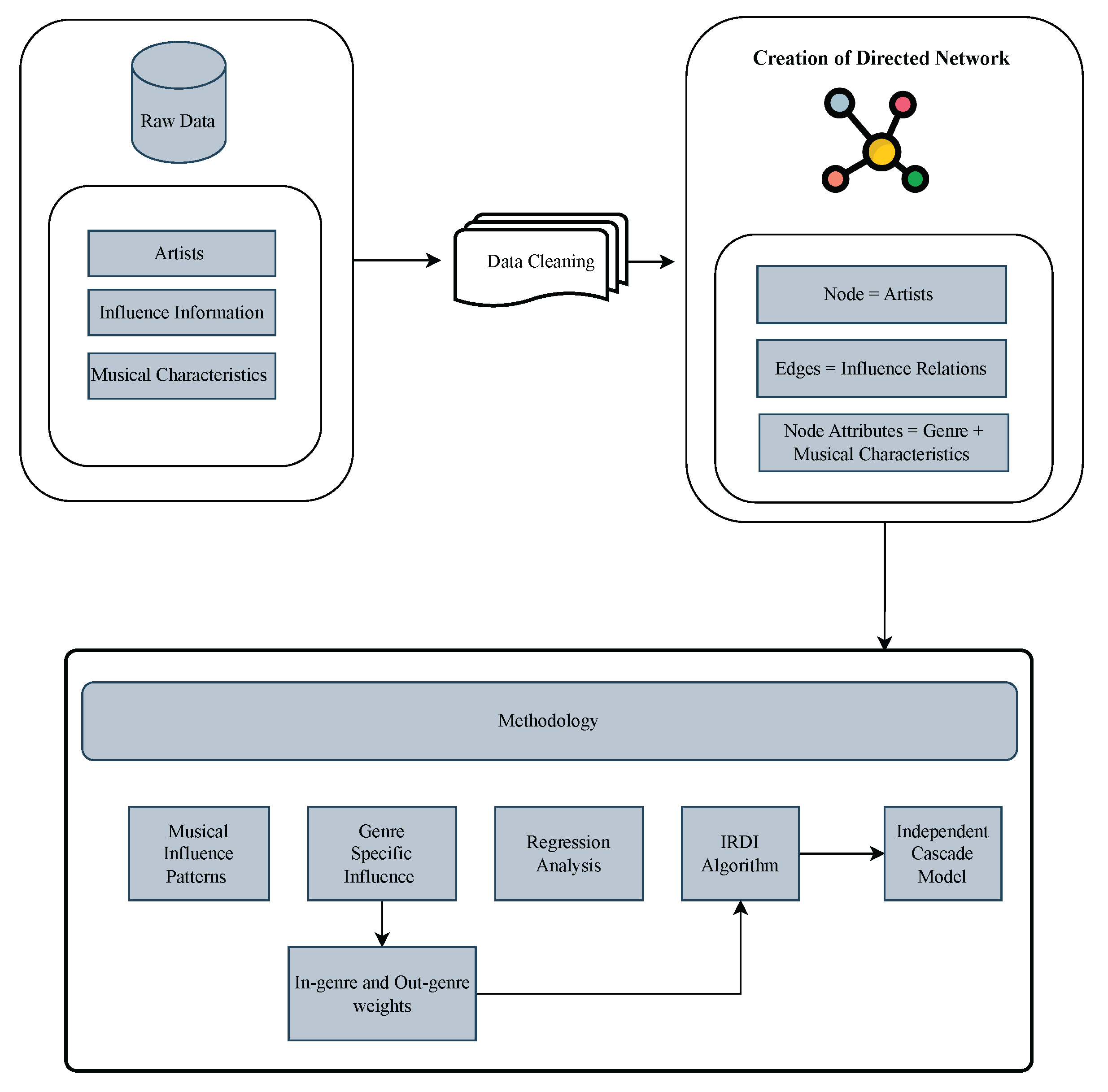
Measuring the extent of the impact within the networks has been the focal point in complex network analysis. This field has diverse practical applications, ranging from social media and technological ecosystems to our specific focus: networks of musical influence. Manaktala and Kumar [13] explored the complexity of a weighted directed social network. They employed triangular fuzzy numbers (TFNs) to measure edge-weight uncertainty. Their research highlighted how fuzzy set theory can effectively assess the strengths of relations. Rui et al. [14] introduced the reversed node ranking (RNR) algorithm in their study, aiming to enhance influence within social networks. They focused on utilizing a node’s reverse rank information and how it influenced its neighbors. Their research highlighted the importance of computational efficiency, a topic we will explore in our upcoming discussion on the IRDI algorithm.
Engsig et al. [15] unveiled the DomiRank centrality, a metric designed to measure the dominance of nodes by considering a combination of local and global topological factors. DomiRank serves as a tool for identifying network weaknesses, providing valuable perspectives on the structural fragility of intricate systems. The similarity between DomiRank and our proposed IRDI algorithm lies in their mutual focus on both local and global information, although applied in different contexts. Mandyam Kannappan and Sridhar [16] formulated a centrality metric known as DONEX, which originates from a Pareto optimal solution addressing the collective welfare maximization problem. DONEX assesses the concepts of dominance and influence within weighted directed networks. Their work demonstrates the importance of considering both edge and node weights, characteristics that also play a role in our IRDI algorithm. The pioneering research by Kempe et al. [17] established the fundamental principles of influence maximization challenges within social networks. They offered mathematical assurances regarding the selection of influential nodes in a network, paving the way for the quantification of influence across diverse network domains, including networks centered on musical influence.
Ding et al. [18] introduced a realistic independent cascade (RIC) model aimed at more accurately capturing the likelihood of candidate seed nodes being accepted in social networks. They proposed new seeding strategies called R-greedy, M-greedy, and D-greedy, demonstrating their superior performance compared to current state-of-the-art algorithms in experiments conducted on both real-world and synthetic networks. Feng and Chen [19] adopted a distinctive approach by integrating concepts and methodologies from causal inference to examine the identifiability of parameters within extended independent cascade (IC) models. Their research concentrated on exploring more realistic propagation scenarios involving unobservable confounding factors, thereby establishing the groundwork for comprehending parameter identifiability in influence propagation models featuring hidden variables. On a similar note, Wang et al. [20] aimed to address the challenges associated with the traditional influence maximization algorithms, which often struggle with a trade-off between running time and implementation. They presented an enhanced discrete particle swarm optimization algorithm designed for the independent cascade model to strike a balance in this trade-off, showcasing an improved execution speed and superior performance when applied to actual social network datasets.
Each of the above works provides a valuable perspective and methodological framework for comprehending the concepts of influence and concepts of centrality within intricate network systems. None of these studies explicitly tackle the subtleties and distinctive attributes of musical influence networks. Our research aims to bridge this gap by introducing the IRDI algorithm. While past research mainly focused on social and infrastructure networks, our work examines musical influence networks. The IRDI algorithm is particularly crafted to handle the complexities associated with musical attributes and dynamics of influence within these networks. For instance, conventional methods, like edge weights and basic centrality measures, fall short of capturing the complexity of musical influence. The introduction of the dominating influencer concept within the IRDI algorithm introduces a novel perspective on comprehending and quantifying influence. This approach goes beyond mere reach, considering the depth and various aspects of musical attributes, including genre, innovation, and collaboration.

3. Methodology

3.1. Data Sources and Collection

Figure 1 gives an overview of different methods used in the paper, starting from data acquisition. The dataset was sourced from both Spotify [21] and AllMusic [22] and was acquired from Kaggle [23]. The data were used for the COMAP (Consortium for Mathematics and its Applications) 2021 competition [24]. Two distinct categories of data were used in this study. The first category, influence data, encompasses information regarding musical influencers and their followers. These data are derived from the artists themselves, as well as insights from industry experts. They comprise details about influencers and followers for 5854 artists spanning the past 90 years. The second category, data_by_artist, includes individual artists’ genres and musical characteristics. These variables encompass musical features, such as tempo, acousticness, liveness, and energy, and artist-related information, such as the artist name and ID. Detailed definitions for these variables can be found in Appendix A.

3.2. Network Construction

Network data harness the relational structure of data. This study focuses on the influence of musical artists and how their musical characteristics play a role in this influence process. We used different network science tools to unlock the hidden patterns and relationships. First, we started by creating a musical network. A network can be directed or undirected. A directed network is one with each edge having a direction [25]. The NetworkX library converted our tabulated data into a directed graph network. Our network consists of nodes and edges, where nodes represent an individual entity, and the edges represent a relationship between them. Table 1 shows different notations used throughout the paper and more details about the creation of a directed network are discussed below.

Creation of the Directed Network

The musical influence network is conceptualized as a weighted directed graph denoted by G = ( V , E , W ) . Here, V represents the set of vertices where each vertex v i corresponds to an artist or musician, given by V = { v 1 , v 2 , , v n } . The set of directed edges E captures the influence relationships between these artists, formally defined as E = { ( v i , v j ) : v i , v j V , i j } . Each vertex v i is associated with a node weight ϕ ( v i ) , which is a vector encapsulating various musical characteristics of the artist. The edge weights in the graph are defined in the set W, where each weight w i j is the absolute difference between the node weights of the corresponding vertices v i and v j . Mathematically, w i j = | ϕ ( v i ) ϕ ( v j ) | . We describe each artist as a node/vertex and the influence between them as the edge. In our musical network, the direction of an edge is from influencer to follower, thereby representing the influence.
A musical influence network is characterized by multidimensional features that encapsulate several aspects of music and influence for each artist. The comprehensive dataset [24] that includes measures such as danceability implies how suitable a track is for dancing. Similarly, energy provides information on the intensity and activity level of a track. Valance is used to describe the emotional tone, tempo to describe the speed, and loudness to indicate the overall volume of the track. In addition, features like acousticness, instrumentalness, speechiness, duration_ms, and liveness are also included. The meta-information on artist popularity, unique identification numbers(influencer_id and follower_id), names (influencer_name and follower_name), primary genres (influencer_main_genre and follower_main_genre), and the decades they started their music careers (influencer_active_start and follower_active_start) are also embedded into the dataset. These attributes participate in the node weight of the respective artist in our network model. Refer to Appendix A for a complete definition and explanation of these variables.
The strength between two nodes can be represented by the edge weight and calculated using the similarity in musical characteristics between the artists. In converting our influence data into a musical network, we set the musical characteristics as node attributes and the difference between the musical characteristics, such as edge attributes. For example, let us consider musical characteristics as energy. The energy levels of each artist will be their node attribute, and the difference between the energy levels of two connected artists will be their edge attributes. The smaller the difference, the stronger the influence it represents.

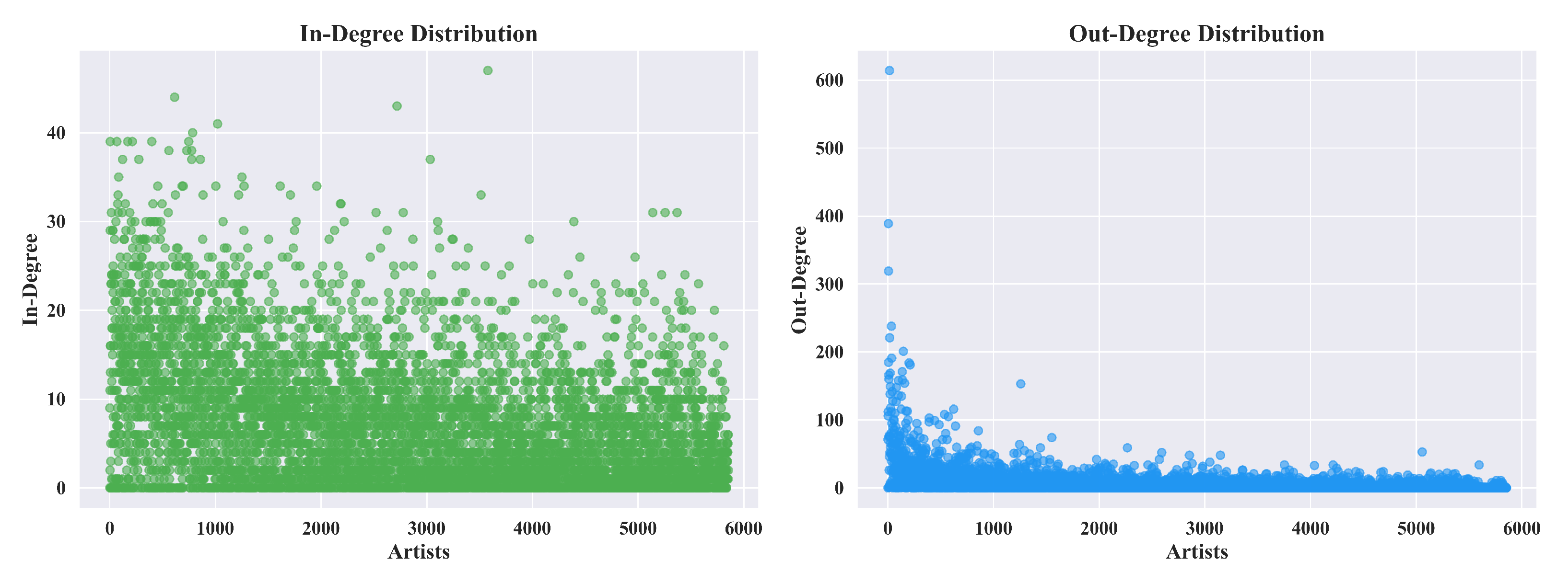
3.3. Fundamental Network Properties

The study of a network can be conducted at the node, edge, and whole network level. In a network, the degree of a node corresponds to the number of other nodes it is connected to or the number of edges connected to it. In the case of a directed network, we investigated the in-degree and out-degree of a node. In our musical network, the in-degree of a node (artist) represents the number of incoming edges or influencers the artist has, and the out-degree represents the number of followers the artist has. A high out-degree for an artist means they have been influential in the musical community.
Assortativity measures the tendency of nodes with similar attributes to connect. It takes a maximum value of “1” on a perfectly mixed network and a minimum value of “ 1 ” when the nodes only connect with nodes of a different type [25]. We calculated the assortativity in our network with respect to the genre of the artists. In the musical network, assortativity measures the tendency of artists to be influenced within their genres. The genre_assortativity for our network is 0.619. Given the relative scale of [ 1 , 1 ] , this moderately high positive value suggests that artists within the same genre tend to be influenced more frequently than expected by chance. Since influence within the genre is expected, the artists that influence artists from other genres contribute more to the overall evolution of the music. We will later quantify this idea of in-genre and out-genre influence.
When analyzing the larger properties of a network, it is crucial to focus on its smaller intricacies. These details help us understand how the dynamics of influence work within the network. Centrality measures provides information on how important or influential specific nodes are within the network. We have employed five different types of centrality measures for this analysis, and their definitions can be found in Table 2.
In our analysis, these centrality measures provide insights into the influence dynamics of artists within the music network. Table 3 summarizes the top 5 artists for each centrality measure. For a detailed mathematical discussion of the centrality measures, please refer to Network by Mark Newman [25].
Degree centrality shows us which artists have the most followers. In our table, we have listed the top 5 artists with the highest degree of centrality. It is no surprise that these artists are considered incredibly influential. However, degree centrality only looks at how many artists they have influenced. To obtain a deeper understanding of our musical network, we are using other centrality measures. Closeness centrality points out artists are closely connected to others. This suggests they are more likely to influence or be influenced by other artists. Interestingly, the artists with high closeness centrality are relatively new compared to those identified by degree centrality. This indicates a diverse range of artists influencing them. Eigenvector centrality identifies influential artists not just because they have many followers but also because of their connections to other influential artists. Betweenness centrality identifies artists who act as bridges in the network. This means they lie in the shortest path between many pairs of artists. Willie Nelson ranks at the top in betweenness centrality. Nelson is credited with helping to create the outlaw country subgenre [9], where he played a role in bridging the gap between country and rock music. The highest betweenness centrality suggests that he has been significant in potentially connecting the traditional country artists with the newer houtlaw generation and, hence, playing an essential role in the transition of country music.

3.4. Empirical Analysis

3.4.1. Musical Influence Patterns

One way to quantify the influence between two artists is by studying how close their musical characteristics are. To calculate the influence of musical characteristics within the influencer–follower pair, we employed a multistep methodology that allowed us to analyze the data comprehensively. Initially, we identified the most influential artists for specific musical characteristics based on the difference value calculated, emphasizing those with the fewest differences. This involved quantifying the differences between these characteristics for each influencer–follower pair, considering smaller differences as indicative of a stronger influence. For instance, we highlighted Mastodon as the most influential acoustic artist, underscoring their unique fusion of acoustic and electric instrumentation. Our analysis also delved into genre-specific trends, revealing how different musical genres exert varying degrees of influence on musical traits.

3.4.2. In-Genre and Out-Genre Influence

Examining the distribution of musical characteristics both within the genres (in-genre) of two artists and outside their respective genres (out-genre) is crucial to understanding the influence of these factors. To determine the in-genre and out-genre distribution, we calculated the number of outgoing edges to an artist within the same genre and outside of the artist’s genre. In-genre influence is defined here as the influence within the artist’s genre, whereas out-genre influence is the impact or influence that the artist has outside of their own genre. This study of in-genre and out-genre influence will help us determine the most influential artists within and outside of the genre and can be studied separately to gain new insight. We applied the weighting factor for both in-genre and out-genre counts to balance their contribution and determined the combined weight. First, we created two subgraphs: in-genre and out-genre. The in-genre subgraph contains all the edges where both the nodes belong to the same genre, while the out-genre subgraph contains the edges where the nodes belong to different genres. The eigenvector centrality for each node in both subgraphs was computed, and the average was taken. We then normalized the two averages to obtain the weights for the in-genre and out-genre influence. We used the weights to calculate the weighted combined influence for every node by multiplying the in-degree influence count by the in-genre weight and adding it to their out-degree count multiplied by the out-genre weight. The steps mentioned below were followed to calculate the combined weight:
  • Partition of graph G into two subgraphs: G in for in-genre influence and G out for out-genre influence.
  • Computation of the eigenvector centrality for each node in G in and G out .
  • Calculation of the average eigenvector centrality for G in and G out as E C in and E C out , respectively.
  • Normalization of the averages to obtain the weights:
    w in = E C in E C in + E C out , w out = E C out E C in + E C out
  • For each node in the network, the weighted combined influence value (WCI) is calculated as
    W C I = I G C · w in + O G C · w out
    where I G C is the in-genre influence count and O G C is the out-genre influence count. These steps were undertaken to ascertain w in and w out for eigenvector centrality; analogously, this methodology is employed to determine w in and w out with respect to different centrality measures.

3.5. Inverse Rank-Dominant Influence (IRDI) Algorithm

Analyzing in-genre and out-genre influences is crucial to understanding an artist’s impact and their role in driving cross-genre music evolution. In this section, we explore the idea of dominating influence and introduce IRDI, a measure to capture the essence of dominating influence in our musical network. The idea is that an artist could be an influencer by influencing many artists, but to be a dominating influencer they must be the top influencer among their followers. The notion of a top influencer is calculated using the difference between the musical characteristics of the follower and the influencer: the smaller the difference, the higher the influence. Consider the artist Frankie Avalon. Frankie’s top 3 influencing artists are Elvis Presley, Frank Sinatra, and Andy Williams, respectively. While Frank Sinatra has influenced Frankie, we see that Elvis Presley has had an even more significant impact on Frankie. These nuanced dynamics, where an artist is not just influencing but they are also the top influencer among many followers, are not captured by current centrality measures. The IRDI fills this gap by accounting for the rank of an artist within the list of top influencers for each follower. This extra layer of study provides a deeper understanding of influence.
We calculated the normed difference in their musical traits to measure the influence between a follower and their influencer. Using the IRDI algorithm, we assigned a score to each artist based on their rank and normed difference from their followers. This algorithm generates an IRDI score for the influencer, where a higher score indicates greater dominance. Our method goes beyond mere ranking. By considering both the rank and the normed difference, the IRDI score reflects the strength of influence concerning musical similarity.
This approach distinguishes and assigns higher scores to influencers with smaller differences, providing a more accurate measure of the strength and significance of their influence. It offers a detailed understanding of dominance in terms of musical influence.
We discussed the importance of incorporating genre while assessing the influence of an artist. Therefore, to include the in-genre and out-genre weights calculated previously and to understand an artist’s impact inside and outside their genre in dominating influence, as shown in Algorithm 1, this algorithm accounts for genre-specific and rank-based dominance influences, providing a deeper assessment.
Algorithm 1: Inverse rank-dominant influence (IRDI).
1:
Initialize dictionary I R D I _ s c o r e s to zero for all nodes
2:
for each node n in Graph G do
3:
   Identify set of influencers I of node n
4:
   Initialize list c h a r a c t e r i s t i c s _ d i f f s
5:
   for each i n f l u e n c e r in I do
6:
     Compute normed difference n d as the Euclidean distance between the musical characteristics of n and i n f l u e n c e r
7:
     Append tuple ( i n f l u e n c e r , n d ) to c h a r a c t e r i s t i c s _ d i f f s
8:
   end for
9:
   Sort c h a r a c t e r i s t i c s _ d i f f s in ascending order of normed difference
10:
   for each tuple ( i n f l u e n c e r , n d ) in c h a r a c t e r i s t i c s _ d i f f s , index i do
11:
     Compute rank as i + 1
12:
     if genre of follower and influencer is different then
13:
        Compute influence score as 0.57 / exp ( r a n k + n d )
14:
     else
15:
        Compute influence score as 0.43 / exp ( r a n k + n d )
16:
     end if
17:
     Add influence score to I R D I _ s c o r e s [ i n f l u e n c e r ]
18:
   end for
19:
end for
20:
Return I R D I _ s c o r e s

3.6. Mathematical Formalism and Complexity Analysis of the IRDI Algorithm

Given a musical influence network represented as a directed graph G = ( V , E ) , where V is the set of artists (nodes) and E is the set of influence relationships (edges), let I n be the set of influencers and F n be the set of followers for an artist n V . We denote V as the total number of artists and D as the average number of influencers per artist. To quantify the influence relationship, the algorithm calculates a scalar influence score for each artist n as follows:
IRDI _ scores ( n ) = m F n W n m e rank n m + nd n m
I n is the set of influencers for artist n; rank n m is the rank of influencer m for artist n; nd n m is the normalized difference between the musical characteristics of n and m; and W n m are the weights calculated in Section 3.4.2, which are either 0.57 or 0.43 depending on whether the genres of n and m are different or the same, respectively.
The mathematical function S ( m , n ) employed in the algorithm is defined as follows:
S ( m , n ) = W e ( rank + nd ( n , m ) )
The core computational steps of the IRDI algorithm can be broken down into three primary operations:
  • Iterating over each artist n in V: O ( V )
  • Evaluating the influence score for an average of D influencers for each artist n: O ( D )
  • Sorting the list of influence scores for ranking, which introduces a complexity of O ( log D )
By combining these complexities, the overall time complexity of the algorithm becomes O ( V · D · ( 1 + log D ) ) . Our examination of the IRDI algorithm in this paper serves as an introductory exploration, with a focus primarily on its application to our specific musical network data. A more exhaustive algorithmic analysis, especially in comparison with other centrality measures, is earmarked for future studies.

3.7. Influence Propagation Analysis in Musical Networks

With a wide range of applications, like viral marketing, behavioral analysis, and information spread, the independent cascade (IC) model [27] provides a framework for analyzing influence propagation. The central idea of the IC model is to mimic how things spread through a network randomly. It also assumes each spreading does not depend on others.

3.7.1. Independent Cascade (IC) Model for Musical Networks

The IC model is predicated on a directed graph G = ( V , E ) . Each edge ( u , v ) E is ascribed an influence probability p ( u , v ) [ 0 , 1 ] , characterizing the likelihood of artist u influencing artist v. Formally, given the musical graph G, the influence probability function p ( . ) on all edges, and an initial seed set S 0 , the IC model engenders the active sets S t for all t 1 via the ensuing randomized operation rule:
The process iterates until a time step t arrives wherein no new nodes are activated, i.e., S t = S t 1 , marking the closing of the diffusion process with the final active set S t [27]. In the Algorithm  2, once a node u is activated at a time step t 1 , it attempts to activate its inactive neighbors at the subsequent time step t with a probability p ( u , v ) , mirroring the likelihood of influence transmission from node u to node v. The process iterates, activating the nodes based on the success of probabilistic influence attempts until it reaches a point where no further activation occurs. This defines the termination of the influence propagation.
Algorithm 2: Independent cascade model for musical networks.
1:
Input: Graph G = ( V , E ) , Influence probabilities p ( . ) , Seed set S 0
2:
Output: Final active set S t
3:
Initialize t = 1 , S t = S 0
4:
while S t S t 1 or t = 1 do
5:
   Set S t 1 = S t
6:
   Initialize S t as a new Set
7:
   for each v S t 1 do
8:
     for each u in N ( v ) ( S t 1 S t 2 ) do
9:
        Perform an activation attempt from u to v with success probability p ( u , v )
10:
        if activation is successful then
11:
          Add v to S t
12:
        end if
13:
     end for
14:
   end for
15:
   Increment t = t + 1
16:
end while
17:
return  S t

3.7.2. Adaptation to Musical Networks

We constructed a directed network graph G with nodes representing artists and edges representing the influence relation among them. This network adopted the independent cascade model. We encapsulated a characteristics vector with the musical attributes of each artist, like danceability, energy, and valence. The normed difference of the characteristics vectors of respective artists was used to determine the influence probability p ( u , v ) on each edge ( u , v ) . We normalized by the maximum norm difference across all edges and subtracted 1 to ensure a higher similarity corresponding to a higher probability of influence:
p ( u , v ) = 1 characteristics ( u ) characteristics ( v ) max ( x , y ) E characteristics ( x ) characteristics ( y )

3.7.3. Comparative Analysis of Seed Sets

The rate and extent of influence propagation are significantly impacted by the initial seed set S 0 . Let us consider two initial seed sets A and B; if seed A reaches all nodes in a shorter time than seed B, it implies that seed A has a higher efficacy in promulgating influence across the network. For example, if the average time for seed set A is 10.03 to populate through all nodes and set B has an average time of 15, this illustrates that seed set A is more efficacious in propagating influence swiftly across the network. This metric serves as a critical benchmark for determining and comparing the potential impact that seed sets have in fostering a widespread influence propagation within the musical network. The difference in propagation speed is dependent on how the network is set and where the seeds are initially placed in the network. The average time for each seed set can provide valuable insights into interpretations of the influence dynamics and the potency of different subsets of nodes in catalyzing a widespread influence propagation within the network.

3.7.4. Regression Approach

In this section, we use regression analysis to demonstrate how musical characteristics play a role in determining an artist’s influence. A similar approach was made by Luo et al. [28], where they used the popularity of the artists as the dependent variable and the musical characteristics as the independent variables. But popularity might not translate to influence [29]. The popularity in the dataset used is calculated based on the total number of plays and how recent those plays are. This will favor the new artists and shadow the old ones. For example, El Guincho has the highest popularity score, followed by Billie Eilish and Harry Styles. While they are popular, they are not considered the most influential. So, to capture this notion of influence, we turn to our network statistics. We used various centrality measures as the response variables for the regression analysis. We computed eigenvector, betweenness, closeness, Katz, and degree centrality using the NetworkX library for influencers’ and followers’ nodes. We used all musical characteristics as an independent variable and used centrality scores as the response variables. Table 4 summarizes the regression models employed.
We used the regression approach to find the coefficients of musical characteristics. We used all the musical characteristics as explanatory variables (independent variables), and centrality scores were used as response variables. We trained five models to find coefficients for each musical attribute for all five centrality scores. Since every centrality score has a different perspective of influence, we used all five centralities to have a model that considers every aspect. We used K-fold cross-validation ( k = 5 ) and Mean Squared Error (MSE) to evaluate our trained models.
K-fold cross-validation: K-fold cross-validation is a resampling procedure used to evaluate machine learning models on a limited data sample. The procedure has a single parameter called k that refers to the number of groups that a given data sample is to be split into. Once the data are divided into these k folds, the model is trained on k 1 folds and tested on the remaining fold. This process is repeated k times, each time with a different fold being the testing set [32]. The final performance measure is the average of the results obtained in each of the k experiments.
For regression problems, MSE measures the average of the squares of the errors or deviations, i.e., the difference between the estimator and what is estimated [32]. It gives how well the model’s predictions match the actual values.
MSE = 1 n i = 1 n ( y i y ^ i ) 2

4. Results

The findings from the network analysis of our musical network, as illustrated in Figure 2, are detailed in this section.
Figure 3 presents the in-degree and out-degree distributions of nodes. The graphs indicate that many artists have relatively lower in-degree values than out-degree values, suggesting the presence of numerous independent artists or those with limited influence. This observation aligns with the network graph in Figure 2, where several nodes have only one connection. However, a few artists serve as “hubs” or essential nodes in the network, as evident from their high out-degree values and their role in connecting multiple other nodes. Notably, the out-degree distribution exhibits higher values compared to the in-degree distribution. This suggests that influencers exert more influence than the extent to which followers engage in following behaviors.

4.1. Musical Influence Patterns

First, we analyze the distributions of differences in musical characteristics for all influencer–follower pairs to understand how each musical feature is being influenced. Table 5 lists the most influential artists with the least differences, where a smaller difference signifies a stronger influence. Mastodon, an American heavy metal band known for their complex and intricate music that combines acoustic and electric instrumentation, emerges as the most influential artist for acousticness. Bappi Lahiri, an Indian artist recognized for his disco and Bollywood style of music, is the most influential artist in terms of energy. His music is characterized by a high energy and upbeat rhythms. David Foster, known for his music genre that encompasses classical, pop, and film scores, is the most influential artist for speechiness, suggesting that his music focuses more on song melodies and harmonies rather than spoken words or lyrics. Table 5 highlights the most influential artists for other musical characteristics as well.
The sum of absolute differences between musical characteristics for each influencer–follower pair was calculated to determine the musical characteristics and how they change between an influencer and a follower. Table 6 shows the absolute differences between musical characteristics for each influencer pair.
The results suggest that speechiness is preserved the most between an influencer and a follower, while duration is preserved the least. However, this only provides an “average” picture. The high difference in duration could be because of the changes in production or consumption habits of the audience, which change over time. The smaller average difference suggests that the follower’s music is like the influencers of that musical characteristic, indicating a strong influence. Genre-specific trends for the absolute difference for musical characteristics was analyzed to determine which genre strongly influences the specific musical characteristics of their followers. Table 7 summarizes the results.
Country music has the lowest sum of difference for danceability, suggesting that danceability is passed down strongly through country artists. Country music often features rhythms that encourage dance, such as line dancing [33]. Valence describes the musical positiveness conveyed by a track, and the smallest valence difference for reggae indicates that reggae artists maintain similar positive and uplifting moods in their songs, which reggae music is known for. R&B is known for soulful melodies and strong beats, consistent with our results for tempo and loudness. These results reveal that genre also affects how two artists influence musical characteristics.
Figure 4 provides a detailed picture of differences in musical characteristics with respect to the genres. Each cell represents the average difference for the characteristics in a specific genre. The values are normalized using MinMaxScaler, where the low values mean a higher influence in the given characteristics by artists of that genre.

4.2. Impact of In-Genre and Out-Genre Influence

Table 8 and Table 9 show the sorted list of artists who have been most influential outside and inside their genre. Artists’ possession of a high out-genre influence implies that they can inspire and affect musicians of different genres. These out-genre influential artists play a vital role in creating new subgenre and musical styles, enhancing the musical history and future and reaching out to a broader audience as they can resonate with listeners across different genres. Influencing outside of one’s genre also benefits an artist’s career through popularity, album sales, and concerts. In addition, a high out-genre influence suggests that artists have transcended their genre and impacted the broader cultural landscape. We also noticed that these influencers make their music timeless and reach new generations of listeners, receiving accolades, awards, and critical acclaim, further boosting their reputation and legacy. Out-genre analysis identifies the artist that has most impacted the musical industry. At the same time, genre influence, as represented in Table 9, shows how much impact that artist has been making in their genre. In comparison to out-genre influence, there is a significantly higher number of influences inside the genre, which suggests that it is comparatively easier to influence within an artist’s genre.
We can observe that Hank Williams has influenced 87 other artists outside of his genre (Table 8). Hank William is known to be the most influential artist of the 20th century in the musical genre of country. Similarly, Muddy Water is an American blues singer known as the father of modern Chicago blues. It is interesting to observe that Muddy Waters had influenced more outside of his genre than in his own genre. This was because his music was the most influential to famous rock bands and guitar players, like Mick Jagger, Jimmy Page, and Eric Clapton. Other enlisted artists that can influence other genres are Kraftwerk, James Brown, and Howlin’ Wolf, and on the list, we have Bob Dylan, who is one of the most influential artists inside his genre, implying his ability to dominate not only his genre of music but also to inspire other musicians. Our in-genre analysis shows that the most influential music belongs to the rock and pop genre, with artists like the Beatles, Bob Dylan, and Rolling Stones being in the top three of our lists with in-genre influence values of 553, 322, and 304, respectively.
Table 10 shows the in-genre and out-genre weights for different centrality measures. This weight shows the importance of the type of influence in the network. Eigenvector, betweenness, and Katz centrality have a higher out-genre weight. Closeness and degree centrality are prioritized for in-genre weight because this centrality favors nodes with more connections, and the artist generally has more connections with the artists in their own genre.
Table 11 shows the top 10 artists for different centrality measures after combining both in-genre and out-genre weights. The most influential artists, the Beatles, Bob Dylan, and the Rolling Stones, make it to the top in each centrality measure. Hank Williams makes it to the fourth position in both betweenness and Katz centrality with the fifth position in eigenvector centrality. David Bowie marks his position at the fourth place of the table for degree and closeness centrality; however, his position drops to fifth on betweenness and Katz centrality. Artists like Jimi Hendrix, Marvin Gaye, Miles Davis, and James Brown remain at the top of the list of most influential artists. The unique position of Hank Williams and Led Zeppelin implies their respective influence networks when considering different centrality measures. The results show that the chosen weighting method, combined with different centrality measures, can comprehensively determine the most influential artists across genres. Although analyzing these in and out-genre weights for various centrality measures provides a nuanced idea of influence, we combine all in- and out-genre weights to obtain aggregate in- and out-genre weights. The aggregate in-genre and out-genre weights were 0.43 and 0.57, respectively.
We observed the most influential artists for different centrality measures combined all the weights from those different centralities, and based on that, we created a list of the top 10 most influential artists, shown in Figure 5. Our weighted centrality analysis identified the Beatles as the most influential artist, followed by Bob Dylan and the Rolling Stones. These top three artists were always at the top for all centrality measures. Our top 10 list features artists from various genres and time periods.

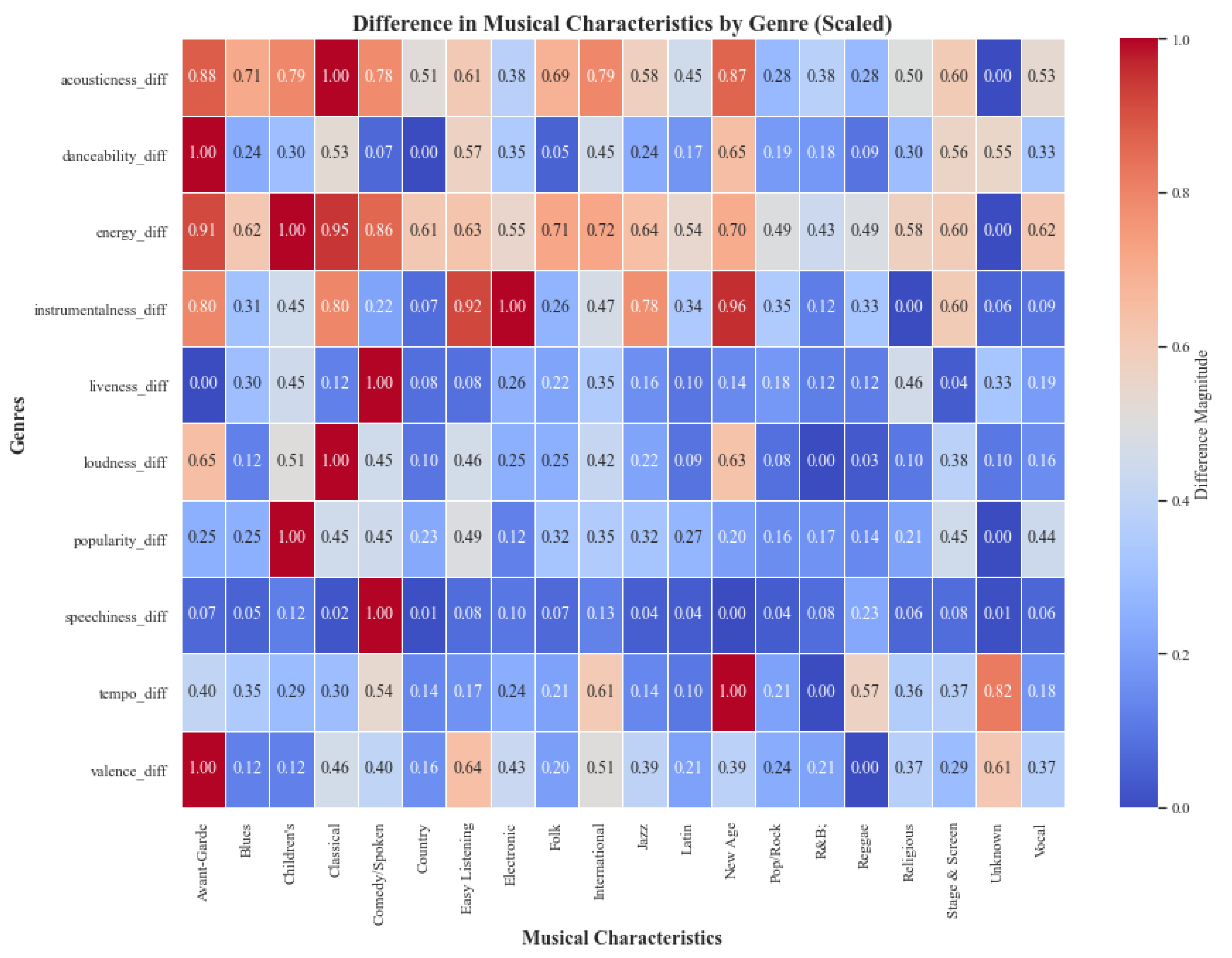
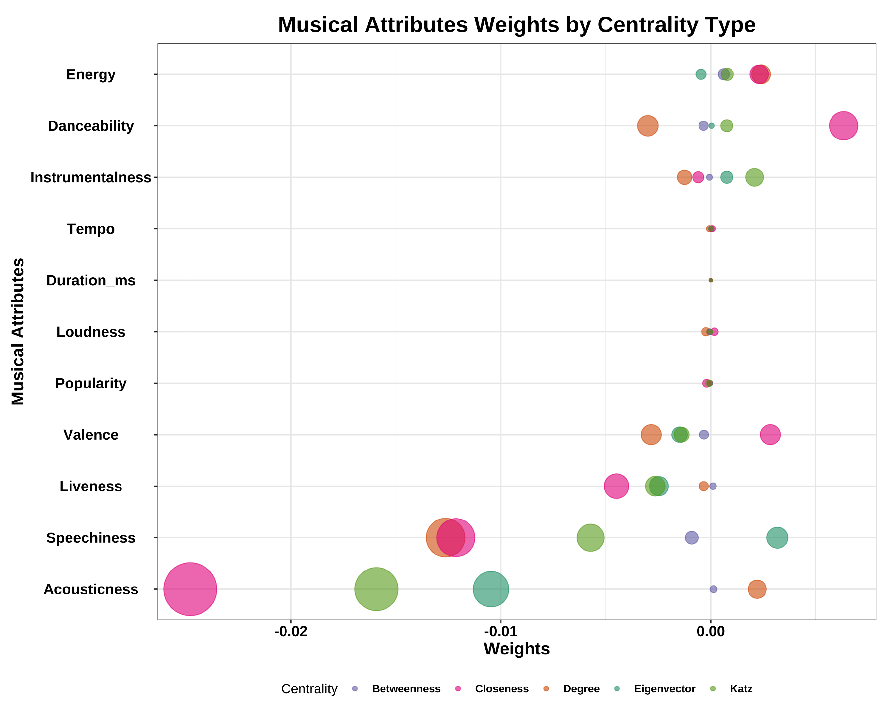
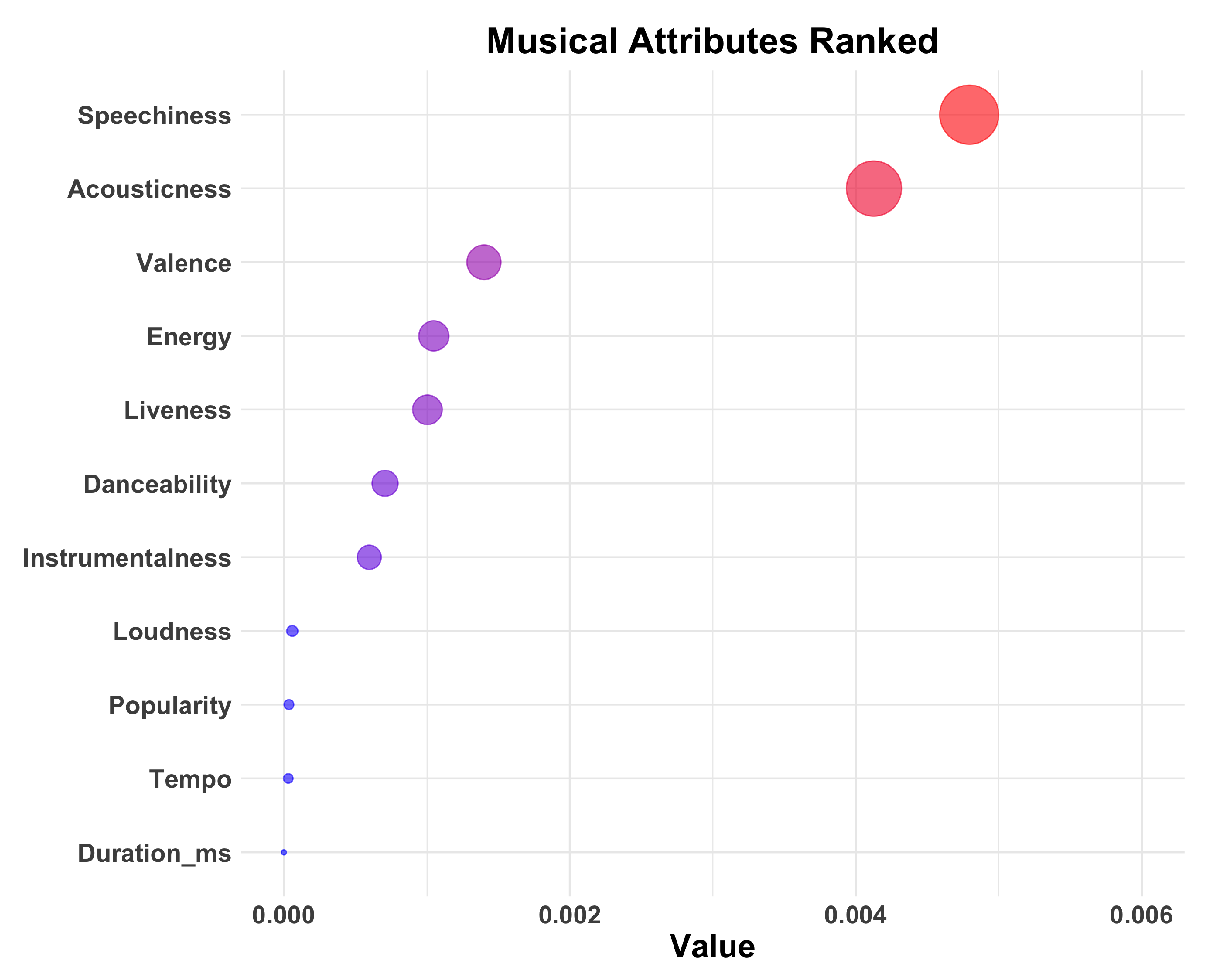
4.3. Impact of Musical Characteristics on Influence

Lasso regression resulted in the lowest MSE overall. However, for the eigenvector centrality the lowest MSE was obtained with Bayesian Ridge regression, and the lowest MSE for Katz centrality was obtained with the linear regression model. Table 12 shows the MSE obtained for all different models.
In Table 12, we obtained the least MSE with a lasso regression model for all centrality types, except for eigenvector and Katz centrality. The idea behind training a model with a centrality type was to understand how each musical characteristic relates to the influence. As we used the centrality measure as the response variable, we trained the model to find the best coefficients for all musical attributes as the explanatory variables. In our model, we trained regression models to predict the centrality scores with the respective centrality of the nodes on either end of an edge in the network, using the difference in attribute weights between the nodes as features. This allowed us to capture the musical attributes’ impact on the importance of the artists.
We obtained five different coefficients for each musical characteristic with respective centrality scores from the regression analysis. While the rankings for each centrality score were not precisely the same, we still noticed some exciting insights; for the most part, we noticed that the order was somewhat preserved. Figure 6 shows that musical attributes are relatively close for each centrality score. For most centrality types, acousticness and speechniess are the essential attributes. Having bigger circles in the visuals implies they are the most important, followed by liveness and valence. Similarly, the least essential attributes were duration, loudness, popularity, and tempo for all centrality types. This provides us with an exciting insight that, regardless of centrality measures, influential artists’ music has a typical trend itself. This leads us to find a score considering each centrality type’s result.
The geometric mean of all the musical attribute coefficients for each centrality type was taken to obtain a grand rank. The intuition behind the geometric mean was motivated by several critical properties that a regular arithmetic mean would have overlooked. These properties included the multiplicative nature, robustness to outliers, scale invariance, interpretability, and preservation of relative importance in accurately combining the measures to represent overall importance. Figure 7 introduces our grand rank.
Figure 7 shows musical attributes that are the most important to the least important with our grand rank. We used centrality scores for our response variable, which helped us determine the influence of the artists; this helped us with characteristics of music that an artist should have to become more influential in most cases. Our grand rank explicitly shows that speechiness, acousticness, and valence are the most critical factors for an artist to become influential. It is also noticeable that duration and tempo are the least important attributes. After that, popularity is also one of the least important attributes, which may be counter-intuitive, as popularity is often seen as a measure of influence. However, as we have used centrality measures to determine the coefficients, this tells us that an artist may be influential without popular songs. This tells us that artists’ general popularity is more impactful than their song’s popularity individually.

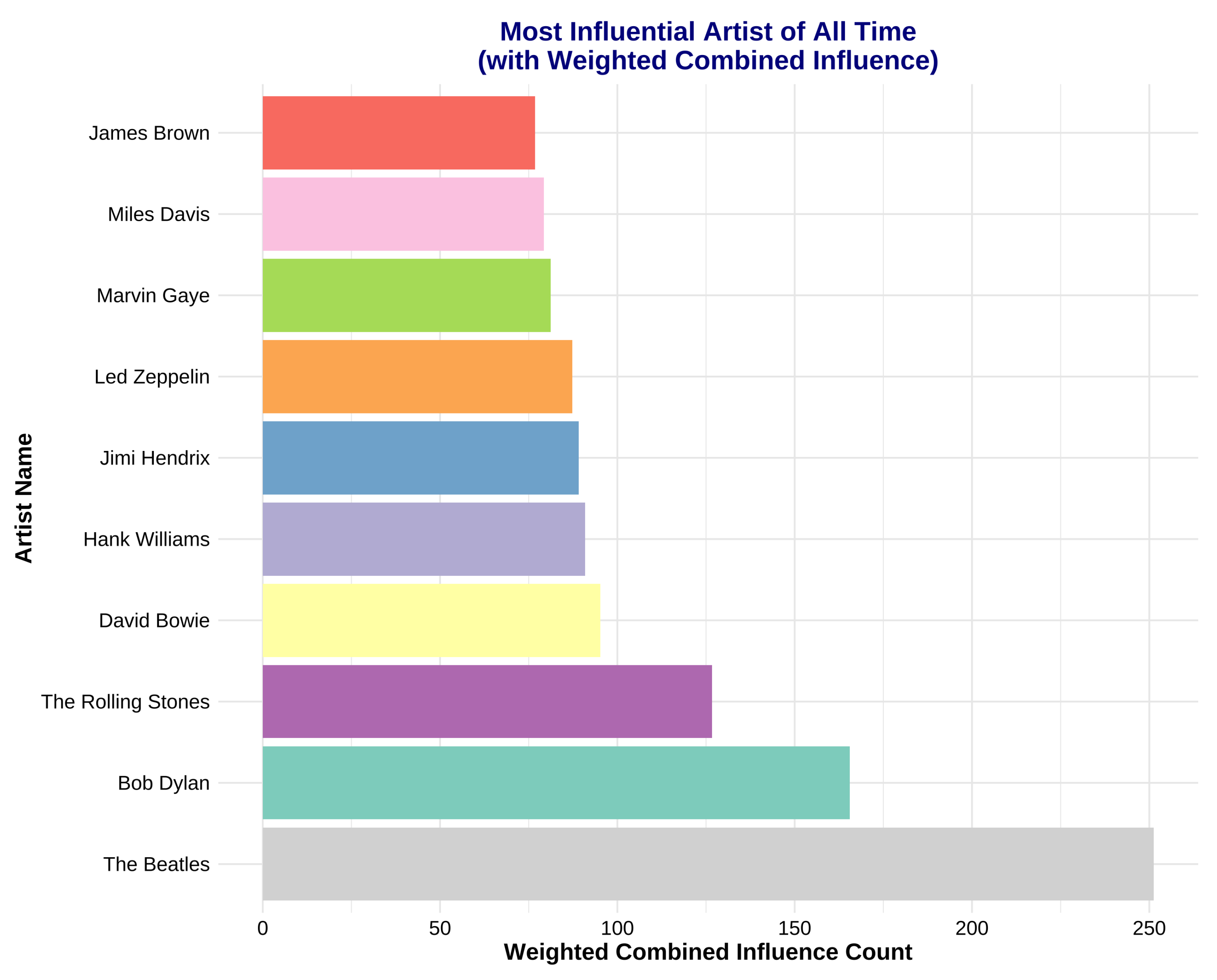
4.4. Dominating Influencers

IRDI scores give us artists that are not just influencers but also dominating influencers. The Beatles led the ranking, followed by Bob Dylan and the Rolling Stones. The Beatles are among the top three influencers with 192 followers, the top two influencers with 130 followers, and the top influencer with 65 followers. The top artists identified from the algorithm include the Beatles, Bob Dylan, the Rolling Stones, the Kinks, Ray Charles, Muddy Waters, Chuck Berry, Sam Cooke, Miles Davis, the Beach Boys, Little Richard, James Brown, Jimi Hendrix, the Yardbirds, Usher, Johnny Cash, The Byrds, Billie Holiday, Thelonious Monk, Madonna, Green Day, the Who, Wilson Pickett, Howlin’ Wolf, and Frank Zappa. Artists such as the Beatles, Bob Dylan, and the Rolling Stones consistently rank at the top in most rankings, highlighting their dominance and significant role in music history, redefining the notion that influence extends beyond mere popularity.

4.5. Propagation Time Analysis

The IC model simulation used seed sets compiled from different sources. These sources include ranking based on various centrality measures, like degree centrality, closeness centrality, betweenness centrality, and eigenvector centrality. Additionally, the simulation used seed sets generated by the IRDI algorithm and a reference set containing the top influencers listed in Zhang et al.’s [6] work. Each seed set comprises the top five most influential nodes for the specific strategy. Table 13 below presents the average time to reach all nodes for various seeding strategies:
A closer examination of the results indicates that the eigenvector centrality seeding strategy yields the fastest propagation with an average of 2.00 steps, followed by closeness centrality with an average of 3.00 steps. These strategies potentially facilitate a quicker influence spread due to the position of the seeds in the network. In the case of eigenvector centrality, the seeds are likely part of a dense subnetwork where the influence can rapidly cascade through highly interconnected nodes. Similarly, the seeds chosen based on closeness centrality are likely positioned in a manner that minimizes the distance to all other nodes, thereby speeding the propagation process.
On the contrary, the betweenness centrality strategy displayed the slowest propagation, averaging 15.24 steps. This approach identifies seeds that serve as bridges between different network segments. As a result, the influence must traverse through these bridge nodes to reach other parts of the network, potentially causing a delay in propagation. Degree centrality and the IRDI algorithm showed similar propagation times of 10.88 and 10.22 steps, respectively. It is possible that the nodes selected as seeds in these strategies, while influential, may not be optimally positioned to expedite the spread of influence across the entire network. They are likely central nodes but may lack connections that span diverse network communities, necessitating more steps for the influence to propagate across the entire network.

5. Discussion

Music has had an ubiquitous presence throughout the world since time immemorial. In one form or another, to this day, music has remained a medium that allows expressions of the seemingly inexpressible and helps an artist convey the extremes and changes in human emotions. This necessitates carefully studying music, its creators, the different forms or genres, and its inspirations and impacts.
Our study comprehensively analyzes the musical influence network from multiple perspectives. Through centrality measures, we identified influential artists, like the Beatles, Bob Dylan, and the Rolling Stones, who consistently ranked at the top. However, centrality alone does not fully capture influence. In addition, in-genre and out-genre data were used to determine influential artists within and outside the genre, and Hank Williams was found to be the most influential artist to impact other genres. This provides a new perspective to analyze today’s music industry and surmise which artists have the most influence to attract an audience outside of their genre. The results presented about the most influential artist of all time with weighted combined influence has an important implication for understanding an artist’s musical impact and influence over different genres. A weighted balanced count presented a comprehensive outlook on artist influence compared to in-genre and out-genre influence counts. Examining the impact of musical characteristics through regression analysis revealed critical attributes, like speechiness, acousticness, and valence.
The IRDI algorithm reveals a different angle into the landscape of musical influence by adding a layer of subtle shade when compared to existing methodologies. Zhang et al. [6] utilize a directed network model along with four different models to investigate musical influence. They used the “NI” metric that combines both network reach and authoritative evaluations to rank influential musicians. Their top influential artists are the Beatles, Chuck Berry, Bob Dylan, Hank Williams, and Little Richard.
Incorporating the weights emphasized artists like Ray Charles, Miles Davis, and Billie Holiday, who have made considerable contributions outside their respective genres. Ray Charles contributed to integrating country music, rhythm and blues, and pop music [34]. Artists like Madonna and Green Day are also highlighted by modified algorithms due to the recognition of their out-genre and subculture influence [35].
This study also provides a different perspective in ranking the top influential artists. The Beatles, Bob Dylan, the Rolling Stones, the Kinks, and Ray Charles are our top influential artists. This result includes several observations in common with Zhang et al.’s [6] work. Predominantly, both studies identified the Beatles and Bob Dylan as extremely influential artists. In addition, the IRDI highlights artists like the Rolling Stones, the Kinks, and Ray Charles. These artists are universally recognized but not highlighted in Zhang et al. [6]’s top five list. Our algorithm considered various musical attributes, including the influence and specific musical characteristics that contribute to an artist’s influence.
The incorporation of genres into the algorithm also gave us artists like Green Day and Madonna, both of whom have made valuable contributions in their respective genres while influencing many. The independent cascade model further classified the robustness of the algorithm, offering perception into the spread dynamics of influence, highlighting artist qualities and their importance in shaping the music industry.

6. Conclusions

This study offers a comprehensive exploration into the fascinating realm of musical influence networks using a balanced mix of network science, machine learning, and statistical techniques. Key insights are highlighted through network analysis, identifying influential artists and emphasizing the role of cross-genre artists, such as Hank Williams. Crucial musical features, like speechiness, acousticness, and valence, have been identified as major drivers of influence through regression analysis. A significant contribution includes the IRDI algorithm, quantifying dominance and capturing intricate details. This study also uses the independent cascade model to shed light on influence propagation. Importantly, the research emphasizes the effectiveness of a multidisciplinary approach in understanding musical influence, and the proposed IRDI algorithm paired with musical attributes carves a promising path forward for future exploration into musical styles and listener preferences.
Music today is not merely an art form but an integral part of human reality; it is an essential nourishment to the body and mind. From making sense of the lows in one’s life to accompanying unrestrained happiness, music has become necessary for meaningful living. This paper conducted a nuanced analysis of several aspects of music in its contemporary fashion by deploying concepts of centrality analysis, in-genre and out-genre influence, and inverse rank dominance influence. This analysis establishes that artists who strive to reach a more significant influence impact the trajectories of other artists as well. In the future, it would be interesting to see whether the social environment is the main factor that influences new music development or if it is the other way around.

Author Contributions

Conceptualization, B.L., A.K.S. and S.D.; methodology, B.L., A.K.S., S.D. and U.D.; software B.L., A.K.S., S.D., U.D. and S.S.; validation, C.D.; formal analysis, B.L., A.K.S. and S.D.; investigation, B.L., A.K.S., S.D., U.D. and S.S.; writing—original draft preparation, B.L., A.K.S. and S.D.; writing—review and editing B.L., A.K.S., S.D., U.D., S.S. and C.D.; funding acquisition, C.D. All authors have read and agreed to the published version of this manuscript.

Funding

This research received no external funding.

Institutional Review Board Statement

Not applicable.

Informed Consent Statement

Not applicable.

Data Availability Statement

The data are freely available on COMAP’s website [24].

Acknowledgments

We are deeply grateful to John R. Sullins for motivating us to embark on this study and for his insightful feedback. We also acknowledge Willson Basyal for his thorough review and suggestions for improving the clarity and coherence of our manuscript. Our thanks extend to Joseph Palardy for his review and invaluable suggestions for improvement. We would also like to acknowledge Nathan Myers for proofreading this manuscript and providing feedback to improve the overall quality of this manuscript. Additionally, we appreciate the assistance of Suprinsa Paudyal for her help with graphical suggestions.

Conflicts of Interest

The authors declare no conflict of interest.

Appendix A. Data Variables

Definitions of variables used in this study.
Danceability: A measure of how suitable a track is for dancing based on a combination of musical elements, including tempo, rhythm stability, beat strength, and overall regularity. A value of 0.0 is the least danceable, and 1.0 is the most danceable.
Energy: A measure representing a perception of intensity and activity. A value of 0.0 is the least intense/energetic, and 1.0 is the most intense/energetic. Typically, energetic tracks feel fast, loud, and noisy.
Valence: A measure describing the musical positiveness conveyed by a track. A value of 0.0 is the most negative, and 1.0 is the most positive.
Tempo: The overall estimated tempo of a track in beats per minute (BPM). In musical terminology, tempo is the speed or pace of a given piece and derives directly from the average beat duration.
Loudness: The overall loudness of a track in decibels (dB). Values typically range between −60 and 0 db. Loudness values are averaged across the entire track and are useful for comparing the relative loudness of tracks. Loudness is the quality of a sound that is the primary psychological correlate of physical strength (amplitude).
Acousticness: A confidence measure of whether the track is acoustic (without technology enhancements or electrical amplification). A value of 1.0 represents high confidence the track is acoustic.
Instrumentalness: Predicts whether a track contains no vocals. “Ooh” and “aah” sounds are treated as instrumental in this context. Rap or spoken word tracks are clearly “vocal.” The closer the instrumentalness value is to 1.0, the greater the likelihood the track contains no vocal content. Values above 0.5 are intended to represent instrumental tracks, but confidence is higher as the value approaches 1.0.
Liveness: Detects the presence of an audience in a track. Higher liveness values represent an increased probability that the track was performed live. A value above 0.8 provides a strong likelihood that the track is live.
Speechiness: Detects the presence of spoken words in a track. The more exclusively speechlike the recording (e.g., talk show, audiobook, poetry), the closer to 1.0 the attribute value.
Duration_ms: The duration of the track in milliseconds (integer).
Popularity: The popularity of the track. The value will be between 0 and 100, with 100 being the most popular. The popularity is calculated by algorithm and is based, in the most part, on the total number of plays the track has had and how recent those plays were (integer).
Influencer_ID: A unique identification number given to the person listed as an influencer (string of digits).
Influencer_name: The name of the influencing artist as given by the follower or industry experts (string).
Influencer_main_genre: The genre that best describes the bulk of the music produced by the influencing artist (if available) (string).
Influencer_active_start: The decade that the influencing artist began their music career (integer).
Follower_ID: A unique identification number given to the artist listed as a follower (a string of digits).
Follower_name: The name of the artist following an influencing artist (string).
Follower_main_genre: The genre that best describes the bulk of the music produced by the following artist (string).
Follower_active_start: The decade that the following artist began their music career (integer).

References

  1. Lipe, A.W. Beyond Therapy: Music, Spirituality, and Health in Human Experience: A Review of Literature. J. Music Ther. 2002, 39, 209–240. [Google Scholar] [CrossRef] [PubMed]
  2. Maryprasith, P. The effects of globalization on the status of music in Thai society. Master’s Thesis, Institute of Education, University of London, London, UK, 2000. [Google Scholar]
  3. Manolios, S.; Hanjalic, A.; Liem, C.C.S. The influence of personal values on music taste: Towards value-based music recommendations. In Proceedings of the 13th ACM Conference on Recommender Systems, Copenhagen, Denmark, 16–20 September 2019; pp. 501–505. [Google Scholar]
  4. Welch, G.F.; Biasutti, M.; MacRitchie, J.; McPherson, G.E.; Himonides, E. The impact of music on human development and well-being. Front. Psychol. 2020, 11, 1246. [Google Scholar] [CrossRef] [PubMed]
  5. Hong, J.; Deng, H.; Yan, Q. Tag-based artist similarity and genre classification. In Proceedings of the 2008 IEEE International Symposium on Knowledge Acquisition and Modeling Workshop, Wuhan, China, 21–22 December 2008; pp. 628–631. [Google Scholar]
  6. Zhang, X.; Ren, T.; Wang, L.; Xu, H. Music Influence Modeling Based on Directed Network Model. arXiv 2022, arXiv:2204.03588. [Google Scholar]
  7. Bryan, N.J.; Wang, G. Musical Influence Network Analysis and Rank of Sample-Based Music. In Proceedings of the 12th International Society for Music Information Retrieval Conference (ISMIR 2011), Miami, FL, USA, 24–28 October 2011; pp. 329–334. [Google Scholar]
  8. Wu, H.; Zhang, C. Influence between Music Based on Big Data Analysis. In Proceedings of the 2021 17th International Conference on Computational Intelligence and Security, CIS 2021, Chengdu, China, 19–22 November 2021; Institute of Electrical and Electronics Engineers Inc.: Piscataway, NJ, USA, 2021; pp. 338–342. [Google Scholar] [CrossRef]
  9. Park, D.; Park, J. Bipartite network analysis of sample-based music. J. Korean Phys. Soc. 2023, 82, 719–729. [Google Scholar] [CrossRef]
  10. Mu, W. Influence measurement and similarity research Mathematical model based on data analysis and Smart Computing. In Proceedings of the 2021 3rd International Conference on Artificial Intelligence and Advanced Manufacture, Manchester, UK, 23–25 October 2021; pp. 2315–2320. [Google Scholar]
  11. Raglio, A.; Imbriani, M.; Imbriani, C.; Baiardi, P.; Manzoni, S.; Gianotti, M.; Castelli, M.; Vanneschi, L.; Vico, F.; Manzoni, L. Machine learning techniques to predict the effectiveness of music therapy: A randomized controlled trial. Comput. Methods Programs Biomed. 2020, 185, 105160. [Google Scholar] [CrossRef] [PubMed]
  12. Carlson, E.; Saari, P.; Burger, B.; Toiviainen, P. Dance to your own drum: Identification of musical genre and individual dancer from motion capture using machine learning. J. New Music Res. 2020, 49, 162–177. [Google Scholar] [CrossRef]
  13. Manaktala, A.; Kumar, Y. Measuring fuzzy domination in fuzzy weighted directed social networks. In Proceedings of the International Conference on Computing, Communication & Automation, Greater Noida, India, 5–16 May 2015; pp. 237–241. [Google Scholar]
  14. Rui, X.; Meng, F.; Wang, Z.; Yuan, G. A reversed node ranking approach for influence maximization in social networks. Appl. Intell. 2019, 49, 2684–2698. [Google Scholar] [CrossRef]
  15. Engsig, M.; Tejedor, A.; Moreno, Y.; Foufoula-Georgiou, E.; Kasmi, C. DomiRank Centrality: Revealing Structural Fragility of Complex Networks via Node Dominance. 2023. Available online: https://api.semanticscholar.org/CorpusID:258715008 (accessed on 20 August 2023).
  16. Mandyam Kannappan, S.; Sridhar, U. A Flow-Based Node Dominance Centrality Measure for Complex Networks. SN Comput. Sci. 2022, 3, 379. Available online: https://api.semanticscholar.org/CorpusID:250595899 (accessed on 19 July 2023). [CrossRef]
  17. Kempe, D.; Kleinberg, J.; Tardos, É. Maximizing the Spread of Influence through a Social Network. 2003. Available online: https://api.semanticscholar.org/CorpusID:7214363 (accessed on 18 August 2023).
  18. Ding, J.; Sun, W.; Wu, J.; Guo, Y. Influence maximization based on the realistic independent cascade model. Knowl. Based Syst. 2020, 191, 105265. Available online: https://api.semanticscholar.org/CorpusID:211830346 (accessed on 12 July 2023). [CrossRef]
  19. Feng, S.; Chen, W. Causal Inference for Influence Propagation—Identifiability of the Independent Cascade Model. arXiv 2021, arXiv:2107.04224. Available online: https://api.semanticscholar.org/CorpusID:235790641 (accessed on 20 July 2023).
  20. Wang, B.; Ma, L.; He, Q. IDPSO for Influence Maximization under Independent Cascade Model. In Proceedings of the 2022 4th International Conference on Data-driven Optimization of Complex Systems (DOCS), Chengdu, China, 28–30 October 2022; pp. 1–6. [Google Scholar]
  21. Spotify—Web Player: Music for Everyone. Available online: https://open.spotify.com/ (accessed on 14 June 2023).
  22. AllMusic. Record Reviews, Streaming Songs, Genres & Bands. Available online: https://www.allmusic.com/ (accessed on 14 June 2023).
  23. Kaggle: Your Machine Learning and Data Science Community. Available online: https://www.kaggle.com/ (accessed on 14 June 2023).
  24. COMAP. The Influence of Music. 2021. Available online: https://www.mathmodels.org/Problems/2021/ICM-D/index.html (accessed on 15 June 2023).
  25. Networks—Mark Newman—Google Books. Available online: https://books.google.com/books?hl=en&lr=&id=YdZjDwAAQBAJ&oi=fnd&pg=PP1&dq=newman+networks+an+introduction&ots=V-N06Medou&sig=1i7U_bJ4isCTuPkUBhfuOGNOhjc#v=onepage&q=newman%20networks%20an%20introduction&f=false (accessed on 14 June 2023).
  26. Bloch, F.; Jackson, M.O.; Tebaldi, P. Centrality Measures in Networks. arXiv 2021, arXiv:1608.05845. [Google Scholar]
  27. Chen, W.; Lakshmanan, L.V.S.; Castillo, C. Information and Influence Propagation in Social Networks; Springer: Cham, Switzerland, 2013. [Google Scholar]
  28. Luo, Z.; Chen, Y. A Novel Exploration of Potential Music Influence Based on Graph Theory. J. Phys. Conf. Ser. 2022, 2253, 12017. [Google Scholar] [CrossRef]
  29. Salavaty, A.; Ramialison, M.; Currie, P.D. Integrated Value of Influence: An Integrative Method for the Identification of the Most Influential Nodes within Networks. Patterns 2020, 1, 100052. [Google Scholar] [CrossRef] [PubMed]
  30. Oleszak, M. Regularization in R Tutorial: Ridge, Lasso & Elastic Net Regression. 2019. Available online: https://www.datacamp.com/tutorial/tutorial-ridge-lasso-elastic-net (accessed on 10 August 2023).
  31. Hastie, T.; Tibshirani, R.; Friedman, J. The Elements of Statistical Learning: Data Mining, Inference, and Prediction, 2nd ed.; Springer: New York, NY, USA, 2009; ISBN 978-0-387-84857-0. [Google Scholar] [CrossRef]
  32. Joshi, R.D.; Dhakal, C.K. Predicting type 2 diabetes using logistic regression and machine learning approaches. Int. J. Environ. Res. Public Health 2021, 18, 7346. [Google Scholar] [CrossRef] [PubMed]
  33. Grizzly Rose Blog. Why Country Music Is the Best. Available online: https://grizzlyrose.com/why-country-music-is-the-best/ (accessed on 15 June 2023).
  34. Ray Charles Biography. Available online: https://www.swingmusic.net/Ray_Charles_Biography.html?fbclid=IwAR3_fQNS2yEg5d1dT5URRwW9_AquLvF5-aOQY0Rz7bh1OKMbFeHIwVVZUuI (accessed on 8 September 2023).
  35. Ben Vaughn. Madonna: The Cultural Icon Who Has Influenced Subcultures for Decades. Available online: https://www.benvaughn.com/madonna-the-cultural-icon-who-has-influenced-subcultures-for-decades/ (accessed on 21 July 2023).
Figure 1. Schematic representation of the structured methodology employed in this study. Note: IRDI represents inverse rank-dominant influence.
Bdcc 07 00180 g001
Figure 2. Graphical Representation of the musical network. Node colors represent genres.
Bdcc 07 00180 g002
Figure 3. In-degree and out-degree distribution.
Bdcc 07 00180 g003
Figure 4. Heat map showing the mean difference for each musical characteristic with respect to the genre.
Bdcc 07 00180 g004
Figure 5. Most influential artist of all time with weighted combined influence.
Bdcc 07 00180 g005
Figure 6. Musical attribute weights by centrality type.
Bdcc 07 00180 g006
Figure 7. Grand rank.
Bdcc 07 00180 g007
Table 1. Notation table.
SymbolDescription
GGraph representing the musical network
VSet of nodes in graph G
ESet of edges in graph G
IRDIInverse rank-dominant influence
ICIndependent cascade
p ( u , v ) Probability of influence propagation from node u to node v
S 0 Initial set of seed nodes
S t Set of active nodes at time t
N ( v ) Set of neighbor nodes that can influence node v
max _ norm Maximum possible norm difference used for normalization
d i ( g ) Number of edges of node i in graph g
ρ g ( i , j ) Network distance between node i and node j
ν g ( i : j , k ) Number of geodesic paths between nodes j and k passing through node i
ν g ( j , k ) Total number of geodesic paths between nodes j and k
c deg i ( g ) Degree centrality of node i
c cls i ( g ) Closeness centrality of node i
c KB i ( g , δ ) Katz–Bonacich centrality of node i
c bet i ( g ) Betweenness centrality of node i
c Eig i ( g ) Eigenvector centrality of node i
λ Proportionality factor used in Eigenvector centrality
δ Discount factor in Katz–Bonacich centrality
Length of walks in the Katz–Bonacich centrality
ϵ Error term in regression models
MSEMean Squared Error, a metric to evaluate the regression model’s performance
λ reg Regularization parameter in various regressions
α Mixing parameter between Ridge and Lasso in ElasticNet regression
β 0 , β 1 Intercept and slope coefficients in regression models
O ( · ) Big O notation, denoting computational upper bounds
Table 2. Summary of centrality measures [26].
MeasureDefinitionEquation
DegreeMeasures the number of edges of the node i, reflecting its connectivity or “popularity”. c deg i ( g ) = d i ( g ) n 1
ClosenessBased on the network distance between a node and each other node, extending degree centrality by considering neighborhoods of all radii. c cls i ( g ) = n 1 j i ρ g ( i , j )
EigenvectorThe prestige of node i is related to the prestige of its neighbors. λ c i = j g i j c j
Katz–BonacichA measure of prestige based on the number of walks from node i. Shorter walks are valued more. c KB i ( g , δ ) = δ j g i j
BetweennessMeasures a node’s role as an intermediary in connecting other nodes in the network. c bet i ( g ) = 2 ( n 1 ) ( n 2 ) ( j , k ) , j i , k i ν g ( i : j , k ) ν g ( j , k )
Table 3. Centrality measures of various artists grouped by centrality type.
Degree CentralityCloseness CentralityBetweenness CentralityEigenvector Centrality
The BeatlesJonas BrothersWillie NelsonParamore
Bob DylanAvril LavigneUncle TupeloWe the Kings
The Rolling StonesHilary DuffPhosphorescentDisturbed
David BowieMeghan TrainorHoyt AxtonFlyleaf
Led ZeppelinDemi LovatoThe Kingston TrioThirty Seconds to Mars
Table 4. Regression models summary [30,31].
ModelDescriptionEquation
LinearBasic linear model. y = β 0 + β 1 x + ϵ
RidgePenalizes the sum of squared coefficients (L2 penalty). y = β 0 + β 1 x + λ β 2 + ϵ
LassoPenalizes the sum of absolute values of the coefficients (L1 penalty). y = β 0 + β 1 x + λ | β | + ϵ
ElasticNetA convex combination of Ridge and Lasso. y = β 0 + β 1 x + λ ( ( 1 α ) β 2 + α | β | ) + ϵ
Bayesian RidgeLinear with Bayesian regularization.Varies by priors.
Table 5. The most influential artist for musical characteristics with the least differences.
CharacteristicsMost Influential Artist
AcousticnessMastodon
DanceabilityZedd
Duration (ms)Caron Wheeler
EnergyBappi Lahiri
InstrumentalnessGavin DeGraw
LivenessMiles Davis Quintet
LoudnessEaston Corbin
PopularityEd Bruce
SpeechinessDavid Foster
TempoMartin Gore
ValanceFreda Payne
Table 6. Differences between musical characteristics for each influencer pair.
Musical CharacteristicsAbsolute Difference
Speechiness0.028
Liveness0.084
Danceability0.097
Instrumentalness0.124
Energy0.149
Valance0.150
Acousticness0.188
Loudness3.109
Popularity9.774
Tempo14.137
Duration58,797.095
Table 7. Musical characteristics with the lowest difference in different genres.
Musical CharacteristicsLowest Difference Genre
DanceabilityCountry
EnergyUnknown
ValenceReggae
TempoR&B
LoudnessR&B
AcousticnessUnknown
InstrumentalnessReligious
LivenessAvant-garde
SpeechinessNew age
DurationUnknown
PopularityUnknown
Table 8. Most influential artists influencing outside of their genre.
ArtistIn-GenreOut-Genre
Hank Williams9787
Muddy Waters3380
Miles Davis8377
Kraftwerk3177
James Brown7876
Howlin’ Wolf2574
Billie Holiday3472
Marvin Gaye9970
Ray Charles4469
Bob Dylan32267
Table 9. Most influential artists influencing their genre.
ArtistIn-GenreOut-Genre
The Beatles55361
Bob Dylan32267
The Rolling Stones30415
David Bowie22414
Led Zeppelin2138
The Kinks1910
The Beach Boys1796
The Velvet Underground1756
Black Sabbath1692
The Byrds1535
Table 10. In-genre and out-genre weights for different centrality measures.
Centrality MeasureIn-Genre WeightOut-Genre Weight
Eigenvector centrality0.390.61
Betweenness centrality0.340.66
Closeness centrality0.560.44
Degree centrality0.560.44
Katz centrality0.350.65
Table 11. Top ten artists using combined weights for each centrality measure.
EigenvectorBetweennessKatzDegreeCloseness
The BeatlesThe BeatlesThe BeatlesThe BeatlesThe Beatles
Bob DylanBob DylanBob DylanBob DylanBob Dylan
The Rolling StonesThe Rolling StonesThe Rolling StonesThe Rolling StonesThe Rolling Stones
David BowieHank WilliamsHank WilliamsDavid BowieDavid Bowie
Hank WilliamsDavid BowieDavid BowieLed ZeppelinLed Zeppelin
Jimi HendrixJimi HendrixJimi HendrixThe KinksThe Kinks
Led ZeppelinMarvin GayeMarvin GayeJimi HendrixJimi Hendrix
Marvin GayeMiles DavisLed ZeppelinThe Beach BoysThe Beach Boys
Miles DavisLed ZeppelinMiles DavisThe Velvet UndergroundThe Velvet Underground
James BrownJames BrownJames BrownBlack SabbathBlack Sabbath
Table 12. Node level characteristics with best machine learning model for least MSE.
CharacteristicsMean Squared ErrorRegression Model
Eigenvector centrality1.10 × 10 5 Bayesian Ridge regression
Degree centrality7.82 × 10 5 Lasso regression
Betweenness centrality3.79 × 10 6 Lasso regression
Closeness centrality3.49 × 10 4 Lasso regression
Katz centrality1.17 × 10 4 Linear regression
Table 13. Performance comparison among different rankings.
Seed SetAverage Time to Reach All Nodes (Steps)
Degree centrality10.88
Closeness centrality3.00
Betweenness centrality15.24
Eigenvector centrality2.00
IRDI algorithm10.22
Zhang et al. [6]10.52
Disclaimer/Publisher’s Note: The statements, opinions and data contained in all publications are solely those of the individual author(s) and contributor(s) and not of MDPI and/or the editor(s). MDPI and/or the editor(s) disclaim responsibility for any injury to people or property resulting from any ideas, methods, instructions or products referred to in the content.

