Evaluation of Short-Term Rockburst Risk Severity Using Machine Learning Methods

Abstract

In deep engineering, rockburst hazards frequently result in injuries, fatalities, and the destruction of contiguous structures. Due to the complex nature of rockbursts, predicting the severity of rockburst damage (intensity) without the aid of computer models is challenging. Although there are various predictive models in existence, effectively identifying the risk severity in imbalanced data remains crucial. The ensemble boosting method is often better suited to dealing with unequally distributed classes than are classical models. Therefore, this paper employs the ensemble categorical gradient boosting (CGB) method to predict short-term rockburst risk severity. After data collection, principal component analysis (PCA) was employed to avoid the redundancies caused by multi-collinearity. Afterwards, the CGB was trained on PCA data, optimal hyper-parameters were retrieved using the grid-search technique to predict the test samples, and performance was evaluated using precision, recall, and F1 score metrics. The results showed that the PCA-CGB model achieved better results in prediction than did the single CGB model or conventional boosting methods. The model achieved an F1 score of 0.8952, indicating that the proposed model is robust in predicting damage severity given an imbalanced dataset. This work provides practical guidance in risk management.

1. Introduction

Deep underground engineering is becoming more common in mine production, tunnel construction, and the construction of various subsurface structures. This trend has led to more frequent encounters with highly stressed geological conditions [1]. As a result, the seismically triggering environment has led to numerous geological hazards, such as rockbursts. A rockburst is a progressive failure process wherein a rock mass ruptures due to the sudden release of a large quantity of stored elastic energy in highly stressed rocks. Casualties and the failure of engineering structures then result from the sudden ejection of surrounding rocks [2]. Rockbursts are becoming more prevalent worldwide as mines delve deeper; as a result, accidents are becoming more common [3]. In central Europe, 42 seismically active mines reported approximately 190 rockbursts that caused 122 casualties over the last two decades [4]. Deep gold fields in western Australia and the Beaconsfield mine in Tasmania have also experienced fatalities [3]. The Taiping head-race tunnels in China have experienced over 400 rockburst incidents, resulting in several casualties and the destruction of mechanical equipment [5]. Numerous countries have faced rockburst problems in mines, tunnels, shafts, and caverns [6,7]. To ensure the safety of personnel, various approaches have been implemented for the real-time monitoring of short-term rockburst risk.

Microgravity, electromagnetic radiation, acoustic emissions, and microseismic monitoring (MS) methods are commonly employed to generate early warnings of short-term rockburst risk [8,9]. Among these techniques, the MS technique has been extensively used in deep engineering excavation to warn of short-term rockburst risks by studying the results of various multi-parameter MS methods using experimental, probabilistic, and fractal-theory approaches [10,11,12]. For instance, Feng et al. examined the fractal behaviour of the energy distribution of microseismic events during the development of immediate rockbursts. The results indicated that, as the rockburst approached, the daily energy fractal dimension for MS events increased [11]. Additionally, Yu et al. investigated the fractal behaviour of the time distribution of MS events for different intensities of rockbursts. The result indicated that time-fractal characteristics could be used to estimate rockburst intensity and that a smaller time-fractal dimension means a lower intensity [13].

Further, using the MS technique, Chen et al. collated 133 rockburst cases and established a relationship between radiated energy and burst intensity. Based on their criteria, rockburst grades were divided into five types: none, slight, moderate, intense, and highly intense [14]. Feng et al. utilised six MS parameters from real-time monitoring and established an early warning method. The proposed method was able to successfully identify the strain and strain-structure slip burst of the Jinping II hydropower project [10]. Additionally, Alcott et al. established performance criteria for MS source parameters and thresholds for daily decision-making on the ground control. Those criteria were used to help identify seismically affected areas [15]. Lastly, Liu et al. observed that, before more significant events, MS apparent volume and spatial correlation length increased, while the energy index, fractal dimension, and b value decreased [6].

All the aforementioned approaches achieved significant results for the early recognition of rockbursts and could be used in early-warning systems. However, the identification of a globally accepted threshold value for rockburst risk that could apply to different site conditions and the choice of MS parameters indicating the various risk levels without the aid of computer models both remain challenging. As a result, some researchers have used a machine learning (ML) approach to predict rockburst risk. The value of ML methods is that they do not require knowledge of input and output, so they can predict outcomes by studying underlying data patterns without human involvement.

Feng et al. proposed an optimised probabilistic neural network (PNN) method to predict rockburst intensity using real-time MS information. The model integrated two other algorithms to improve performance, which increased the model’s accuracy in predicting test samples by 20% compared to the standard PNN model [16]. Additionally, Liang et al. developed boosting and stacking ensemble methods using real engineering datasets. Those researchers achieved significantly higher accuracy in predicting short-term rockbursts [17,18]. Further, Liu et al. presented an artificial neural network (ANN) for the dynamic updating of short-term rockburst predictions. The model was further optimised by embedding a genetic algorithm (GA), which was employed to predict 31 actual cases. The results showed that the model could correctly estimate 83.9% of rockburst cases [19]. Further, Zhao et al. built a decision tree (DT) model to predict the exact rank of the rockburst using MS information. The relationship between the MS features and rockbursts was investigated using the DT classifier, and the results showed that the model could accurately predict risk and provide insights regarding rockbursts using MS data [20]. Toksanbayev and Adoko collected 254 samples from seismically active mines and established a damage-scale classification model based on multinational logistic regression (LR). The proposed work used regression equations to create probabilistic models for the assessment of seismic hazards in mines [21]. Lastly, Ullah et al. integrated K-means clustering with extreme gradient boosting (XGBoost) [22]. The original data were relabelled through a clustering method, and XGBoost was trained and tested to validate the model.

All the above-mentioned models have contributed significantly to improving the accuracy of prediction. Neural networks have an advantage in dealing with complex nonlinear problems; however, some neural-network models are susceptible to problems caused by irrelevancies in the data and prone to suboptimal local minima. Although the integration of multiple hybrid and complex ensemble models improves prediction accuracy, the resultant models are often difficult to understand and execute. LR and DT are simple and easy to use but have less accuracy in highly complex, nonlinear rockburst problems. Most applied methods have focused on achieving higher accuracy in predicting risk, and the microseismic dataset is comparatively small. The proportions of different intensity levels in datasets are often unequal. However, accurately classifying each risk level is crucial when classes are imbalanced. One previous study [23] shows that the boosting method (CGB) is more efficient for analysing multi-class imbalanced data in small and large datasets than are other boosting algorithms. However, the feasibility of employing CGB in short-term rockburst prediction has never been studied before, and it is necessary to develop a simple and easy-to-use classification model with promise for predicting each class level effectively.

Therefore, this work proposes a PCA-CGB classification model to create a simple and reliable approach to predicting the intensity of rockbursts. The advantage of this proposed work over the previous approach is that more data have been gathered for the study; additionally, variable redundancies are managed through unsupervised learning. Also, to precisely classify each majority or minority class, a simple model is built and performance is comprehensively evaluated using various metrics.

2. Materials and Methods

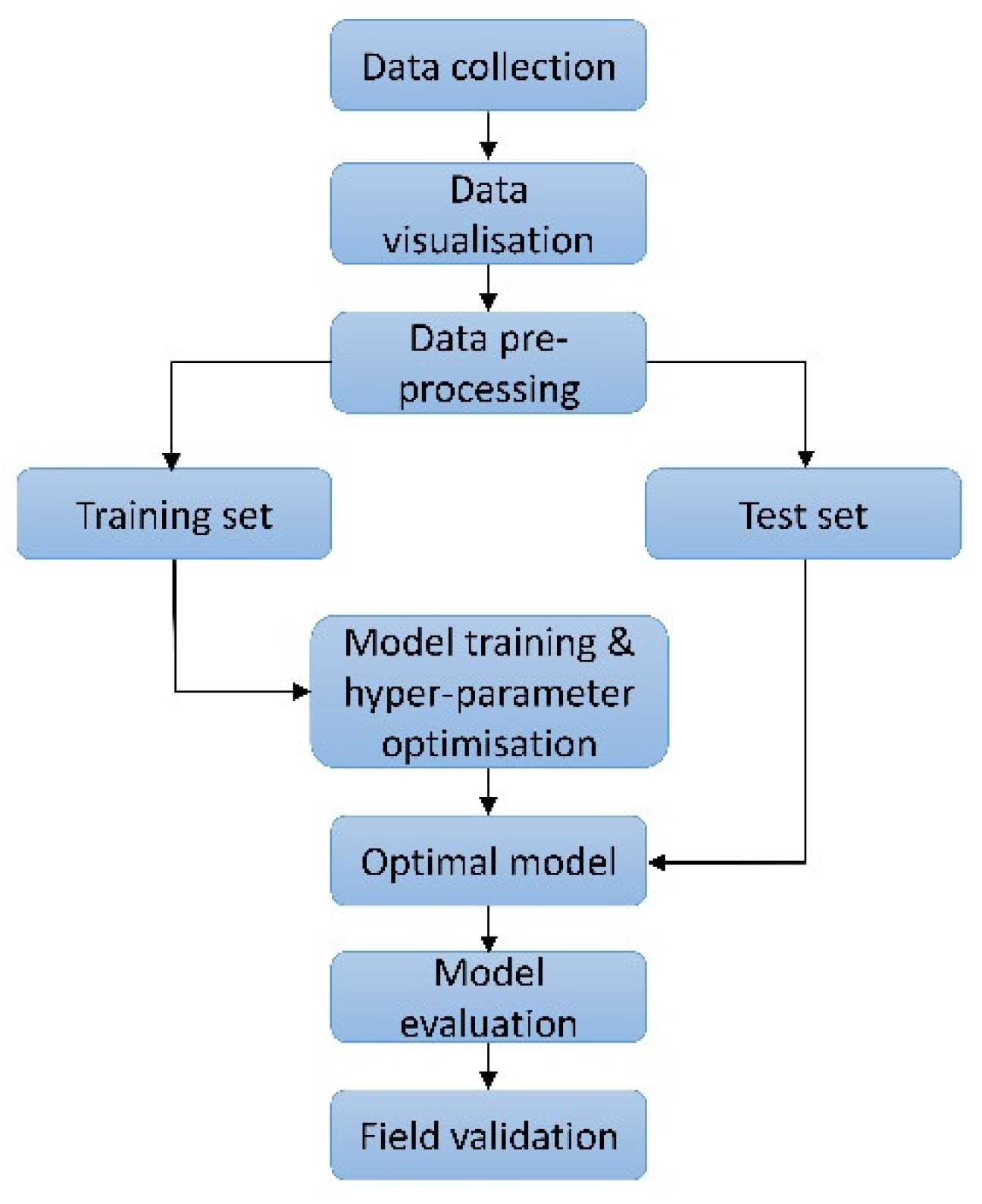
The flowchart of the proposed method is shown in Figure 1.

2.1. Data Collection

Rockburst data were extracted from [19,24] as a supportive database based on microseismic information. All data were obtained from underground tunnelling works and include the following six MS parameters as the feature variables: cumulative MS events (PN), logarithm of cumulative MS energy (PE), logarithm of cumulative apparent volume (PV), event rate (PNR), logarithm of energy rate (PER), and logarithm of apparent volume rate (PVR). Rockburst intensity was the output variable. The output variable has four intensity classes: none (N), slight (S), moderate (M), and intense (I). The classes of the output-variable are described in

Table 1. Descriptions of target-variable classes. Authors’ own work based on [14].

Rockburst Intensity	Characteristics
None	Crack appears inside rock mass; no obvious failure on the surface of rock mass; construction and supports are unaffected
Slight/Weak	Failure is accompanied by slight spalling and slabbing, with slight ejection of rock fragments of size 10–30 cm; failure depth is less than 0.5 m; no harm to the support system and construction if supports are provided at the time
Moderate	Failure of surrounding rock mass followed by severe slabbing and spalling; ejected-fragment size of 30–80 cm; failure sound resembles detonator blasting and lasts for some time; failure depth is more than 0.5 m and less than 1 m; shotcrete lining among rock bolts could be damaged
Intense	Extensive failure range with an ejected-fragment size of 80–150 cm; failure zone with fresh fracture plane; burst sound like an explosive with an impact wave; failure depth between 1–3 m; damage system fully destroyed and severe impact on construction

.

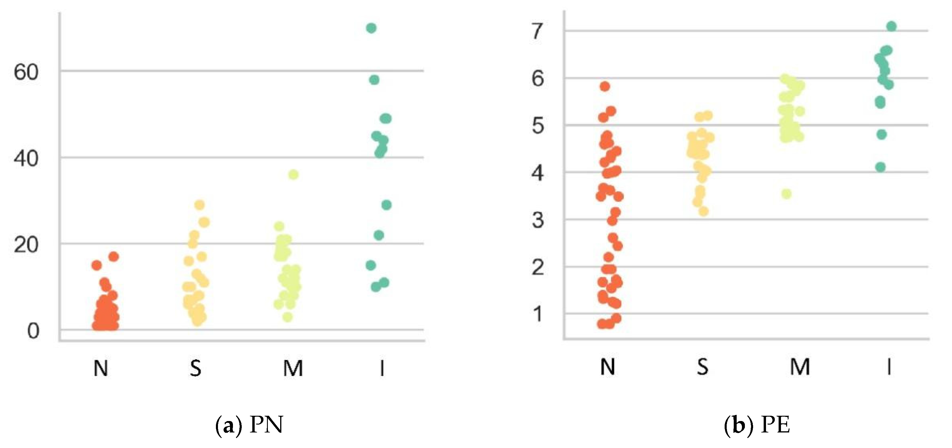
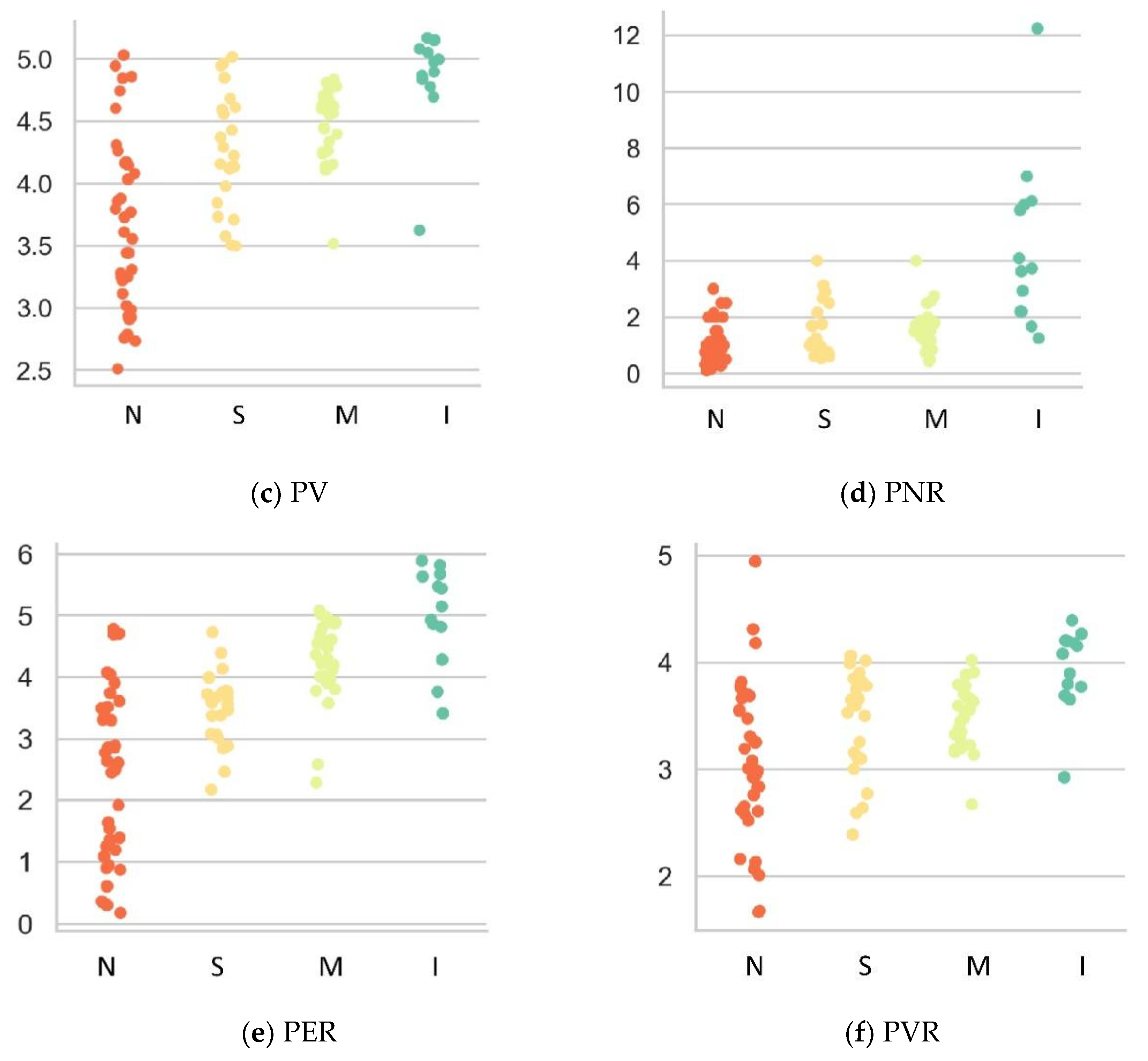
Figure 2 shows the six different features and the distribution of the four intensity levels. In Figure 1, PN represents the density of microfractures. Similarly, PE and PV represent the fracture strength and the degree of damage to the rock mass, respectively. These three parameters are basic parameters that reflect characteristics of microfractures during rockburst development [10]. To account for temporal characteristics in the mechanism, three parameters pertaining to time are considered: PNR, PER, and PVR. PNR reflects the frequency of microseismicity, the failure process of the rock mass, and the average evolutionary law of the response over time. PER represents the microseismic radiation energy of the rock mass per unit of time, and PVR is the volume of the rock in the inelastic zone of deformation per unit of time. The PE, PV, PER, and PVR values are in common logarithmic form to ensure it does not change the correlation of the data variables; the form also compresses the scale of the predictors and reduces the absolute values of the datapoints [17]. The data-acquisition method is reported in [10]. Figure 2 demonstrates that all features contain a degree of discreteness in their characteristic values. For example, we can see that the characteristic values for some intensity class in PN, PV, PNR, and PVR show some discreteness and differ marginally in magnitude. This result arises because some microseismic activity was silent during rockburst development and the microseismic behaviour was stable and low. The precursors of the rockburst were thus not noticeable. When a rockburst occurs, microseismic activity increases suddenly and sharply, so this type of rockburst is not easy to accurately predict in an early-warning system because it is often dispersed [24], reflecting the complex mechanisms of rockburst formation.

2.2. Data Visualisation and Pre-Processing

Data visualisation, analysis, and pre-processing are critical in data science to understanding statistical information, the distribution of variables, the pattern between multivariate features and targets, and the correlation among predictors. This dataset contains 37 none, 26 slight, 23 moderate, and 13 intense rockburst cases. As we can see, the dataset is imbalanced, as the distribution of the four classes is not equal. The classes are in categorical form and, for convenience, are converted into ordinal form by assigning values of 0, 1, 2, and 3 for none, slight, moderate, and intense rockbursts, respectively. The statistical descriptions of each intensity level are summarised in

Table 2. Statistical description of intensity levels across different predictors.

Intensity Class	Predictor Variables
	Statistical Description	PN	PE	PV	PNR	PER	PVR
0	Minimum	1	0.78	2.51	0.11	0.17	1.66
	Maximum	17	5.82	5.03	3.00	4.78	4.94
	Mean	4.16	3.08	3.68	0.98	2.46	3.06
	Standard deviation	3.812	1.47	0.70	0.75	1.35	0.72
1	Minimum	2	3.17	3.49	0.53	2.17	2.39
	Maximum	29	5.20	5.01	4.00	4.72	4.06
	Mean	11.61	4.31	4.25	1.58	3.48	3.42
	Standard deviation	7.96	0.52	0.47	0.97	0.58	0.49
2	Minimum	3	3.54	3.51	0.42	2.28	2.67
	Maximum	36	5.98	4.83	4.00	5.07	4.01
	Mean	14.62	5.24	4.46	1.63	4.22	3.48
	Standard deviation	6.95	0.53	0.29	0.75	0.68	0.29
3	Minimum	70	4.11	3.62	1.25	3.41	2.92
	Maximum	10	7.09	5.16	12.2	5.89	4.39
	Mean	37.31	5.93	4.86	4.52	5.00	3.93
	Standard deviation	18.59	0.80	0.40	2.98	0.78	0.38

Note: PE, PV, PER and PVR are in common logarithmic form.

. Table 2 contains the statistical parameters mean, standard deviation, minimum, and maximum for each of the four classes, and it is possible to determine how their value distribution varies across six different features. For instance, for classes 0 and 3, the minimum and maximum MS energy values range from 0.78 to 5.82 and from 4.11 to 7.09, respectively. Similar comparisons can also be made for other variables using data from the table below.

2.3. Histogram and Parallel Plot

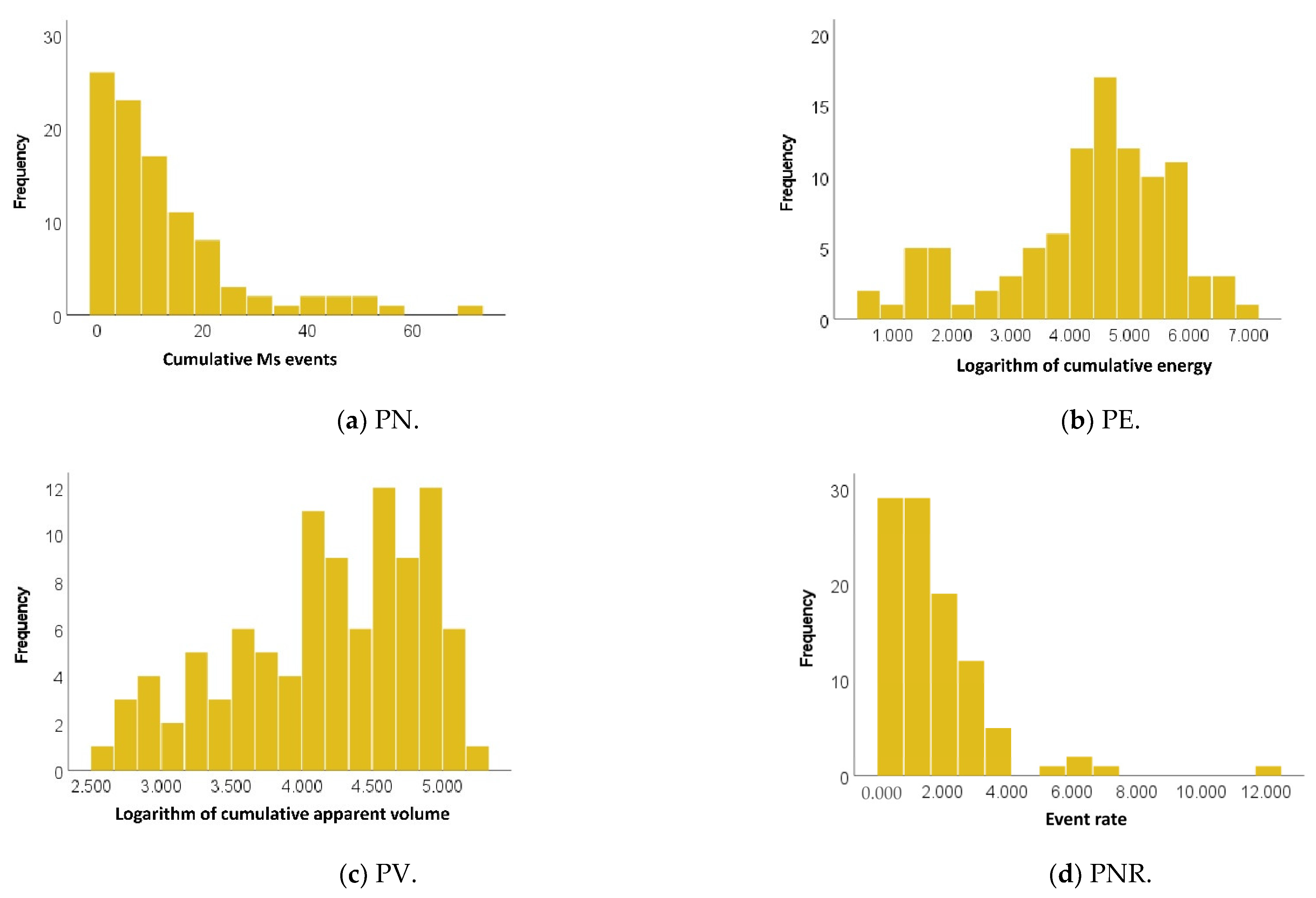
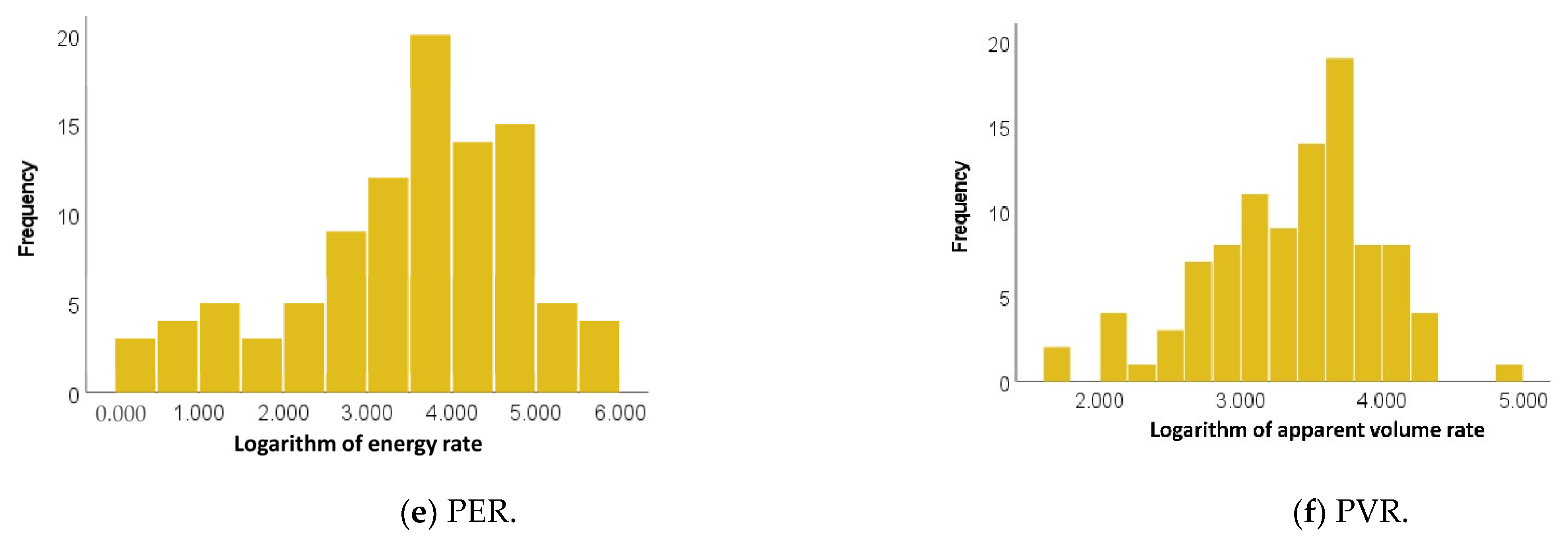
A histogram provides insights into how variables are distributed or whether they are positively or negatively skewed or distorted. According to Figure 3, the values of PE, PER, and PVR resemble a Gaussian distribution, but all are slightly negatively skewed. PN and PNR are positively skewed, and PV is marginally negatively skewed. The scaling of such features often increases the performance of models.

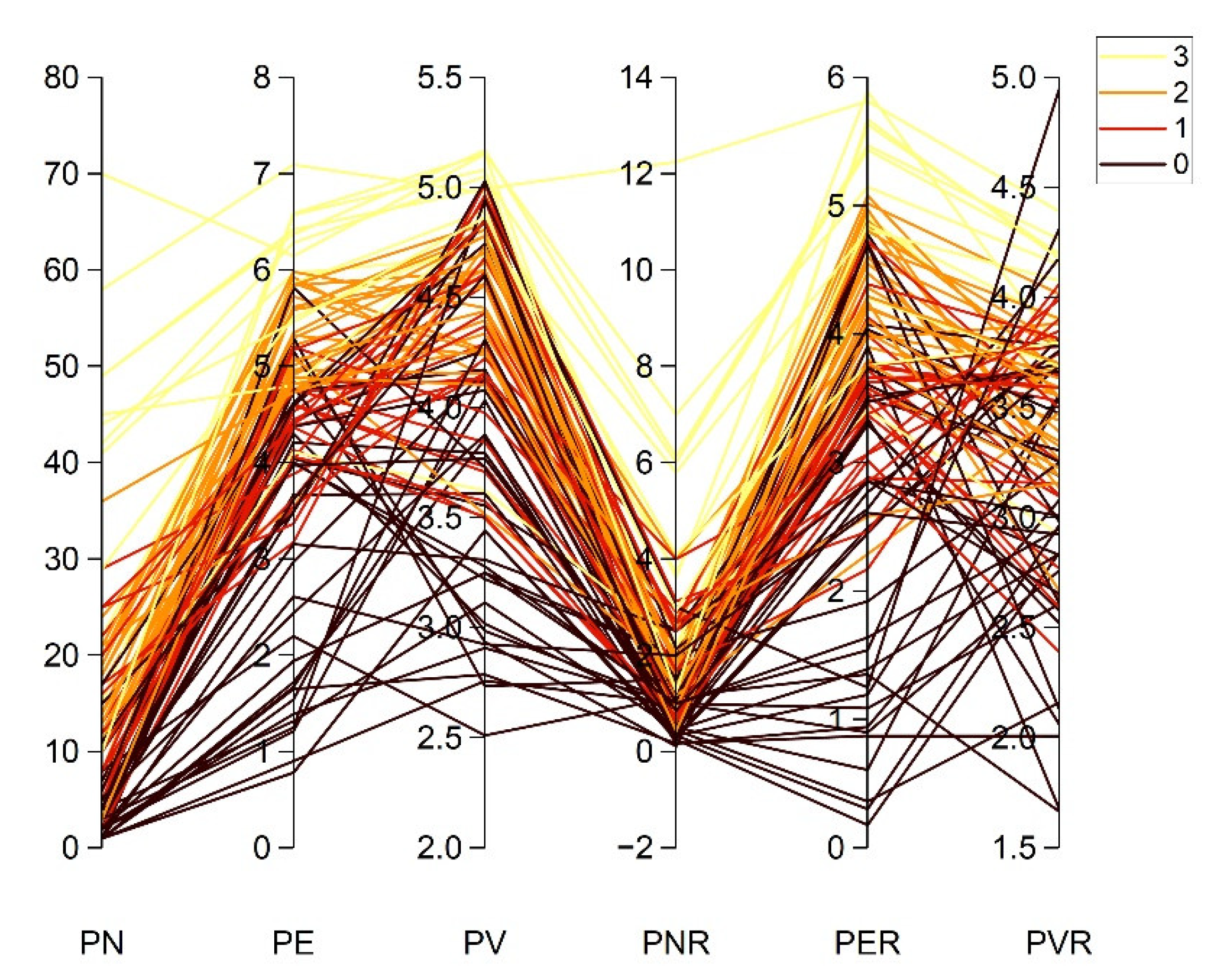
After the descriptions of target and feature variables were individually examined, a parallel plot was used to visualize the underlying relationship between input and output variables, as shown in Figure 4. Parallel coordinate plots aid in comprehending the graphical representation of multivariate MS information [19]. The vertical axis represents each independent variable, and line graphs of different colours represent rockburst grades. Based on the plot, the following conclusions can be reached:

• There is no rockburst when PN and PNR values are low and PE, PV, PER, and PVR values are low-to-medium (dark brown lines).
• Slight and moderate grades have overlapping lines, indicating that medium PN and PNR values and medium-to-high PE, PV, PER, and PVR values are often associated with slight or moderate rockbursts (red and orange lines).
• Medium-to-high PN and PNR values and high PE, PV, PER and PVR values correspond to intense rockbursts (yellow lines).

Figure 4. Parallel plot for MS parameters and rockburst grades.

Figure 4. Parallel plot for MS parameters and rockburst grades.

Overall, it is evident that the relationship between MS parameters and rockburst risk is very complex. It can also be seen that there is some overlap in feature values between slight and moderate rockbursts.

2.4. Correlation Examination

Correlation represents the dependencies between two variables and measures the degree to which one fluctuates in relation to the other. Correlation analysis can categorise into three groups: positively correlated, uncorrelated, and negatively correlated. The Pearson correlation coefficient is often used to compute correlations among variables and is expressed in the following form:

$$r=\frac{\sum (x_i-\overline{x})(y_i-\overline{y})}{\sqrt{\sum {(x_i-\overline{x})}^2\sum {(y_i-\overline{y})}^2}}$$

(1)

Simply, $r$ is a Pearson correlation coefficient and $x_i$ and $y_i$ are the $X$ and $Y$ variable samples. Likewise, $\overline{x}$ and $\overline{y}$ denote the mean values of the $X$ and $Y$ variables, respectively. The $r$ value ranges from ‘−1’ to ‘+1’, and different coefficient values indicate the various degrees of correlation, as depicted in

Table 3. Measure of correlation strength based on Pearson correlation coefficient. Authors’ own work based on [26].

Pearson Correlation Coefficient as an Absolute Value	Correlation Strength
0–0.19	Very weak correlation
0.20–0.39	Weak correlation
0.40–0.59	Moderate correlation
0.60–0.79	Strong correlation
0.80–1.00	Very strong correlation

[25].

2.5. Dimensional Reduction

Principal component analysis (PCA) is a dimensionality-reduction technique that maps higher-dimensional data to a lower-dimensional space through mathematical transformation. The procedure used to conduct PCA follows the standard below [26]:

• Construct the original data matrix $M={\left(x_{ij}\right)}_{m\times n}$, which contains $m$ samples with $n$ variables. $x_{ij}$ is the value of the $j$ predictor for observation $i$.
• Standardise the data to eliminate the effect of varying magnitudes of variables:

  $$x_{ij}^{\ast }=\frac{x_{ij}-{\overline{x}}_j}{s_j}$$

  (2)

  where the mean and standard deviation of the $j$ predictor are denoted by ${\overline{x}}_j$ and $s_j,$ respectively.
• Afterwards, use the standardised data to compute the correlation coefficient matrix $CM={\left(r\right)}_{n\times n}$, where $r$ stands for the Pearson correlation coefficient.
• Compute the eigenvalues and eigenvectors of the $CM$ matrix.
• Choose the appropriate principal components to reduce the original dimension into a lower dimension. Generally, criteria for the first few principal components are eigenvalues greater than 1 and cumulative contribution rate above 80% are elected [26].

The formula provided is used to calculate the contribution rate of the first $p$ principal components:

$${\eta }_p=\frac{{\lambda }_1+{\lambda }_2+\cdots \cdots {\lambda }_p}{{\lambda }_1+{\lambda }_2+\cdots \cdots {\lambda }_n}$$

(3)

where $\lambda$ stands for eigen value.

2.6. Categorical Gradient Boosting Classifier

CGB was initially proposed by [27] because of its usefulness in both classification and regression. CGB has demonstrated superiority over other leading boosting variants that have been applied to different problems. For instance, CGB demonstrated better performance than extreme gradient boosting (XGboost) and light gradient boosting (LGBM) in the work of [27]. Most recently, a comparative study from Wu et al. found that CGB has remarkable predictive capabilities compared with existing boosting methods [28]. It also performed particularly well in some geotechnical areas, such as uniaxial compressive-strength prediction [29] and prediction of the elastic modulus of rocks. Some recent studies have also verified that CGB is superior to other boosting classifiers when applied to multi-class imbalanced data [23].

The working strategy of CGB is to learn many weak learners and integrate them to form a stronger learner. This approach is similar to the strategies of all other boosting methods. It implements gradient boosting with binary decision trees as weak learners [27]. For data with samples $D={\left\{\right(X_j,y_j\left)\right\}}_{j=1,\dots m,}$, $X_j=\left(x_j^1,x_j^2,\dots \dots ,x_j^n\right)$ represents the vector of n number of features and target $y_j\in \mathbb{R}$, which is either binary or a numerical response. Samples ($X_j,y_j$) are independently distributed according to some unknown distribution $P(.,.)$. The objective of the learning task is to train a function $H:{\mathbb{R}}^n\to \mathbb{R}$ that minimises the expected loss, which is provided in Equation (4).

$$\mathcal{L}\left(H\right)≔\mathbb{E}L(y,H\left(X\right))$$

(4)

where $L(.,.)$ represents a smooth loss function and $(X,y)$ represents validation data sampled from $D$.

The process for all iterative gradient boosting constructs a sequence of approximations $H^t:{\mathbb{R}}^m\to \mathbb{R},t=\mathrm{0,1},\dots \dots$. From the previous approximation, $H^{t-1}$, $H^t$ is acquired in an additive process, as $H^{t-1}$+${\alpha g}^t$, with a step size $\alpha$ and function $g^t:{\mathbb{R}}^n\to \mathbb{R}$, which is a base predictor and is chosen from a group of functions G to minimise the expected function defined in Equation (5).

$$\begin{array}{}{g}^t=\arg {min}_{g\in G}\mathcal{L}(H^{t-1}+g)\hfill & =\arg {min}_{g\in G}\mathbb{E}L(y,H^{t-1}\left(X\right)+g(X\left)\right)\hfill \end{array}$$

(5)

The Newton method often deals with the minimisation problem using a second-order approximation of $\mathcal{L}(H^{t-1}+g^t)$ at $H^{t-1}$ or with the help of a gradient step. Further detailed information can also be obtained in [27].

2.7. Evaluation Metrics

Generally, evaluation metrics evaluate the model’s performance in assessing the test sample and whether the classifier can appropriately classify the new observations. Although there are various performance metrics for evaluating classifier robustness, this study adopts three metrics: precision, recall, and F1 score. The primary reason for selecting these metrics is that they are useful for evaluating performance when the dataset has a class-imbalance problem. As mentioned in Section 2.2, the numbers of datapoints in the four classes are not equal, making the classes imbalanced; in this case, the F1 score aids in addressing such problems by weighting precision and recall equally. The accuracy, precision, recall, and F1 score for any classifier is calculated using the following formula:

$$\mathrm{Accuracy}=\frac{\mathrm{T}\mathrm{P}+\mathrm{T}\mathrm{N}}{\mathrm{T}\mathrm{P}+\mathrm{F}\mathrm{P}+\mathrm{F}\mathrm{N}+\mathrm{T}\mathrm{N}}$$

(6)

where true positive (TP) indicates the number of positively predicted observations that are actually positive; false negative (FN) represents the number of negatively predicted observations that are actually positive; false positive (FP) denotes the number of predicted positives that are actually negative; and true negative (TN) is the number of predicted negatives that are actually negative.

Precision measures the correctness of a model’s positive predictions [30]. It is the fraction of predicted positive examples that were actually positive and is provided by:

$$\mathrm{Precision}=\frac{\mathrm{T}\mathrm{P}}{\mathrm{T}\mathrm{P}+\mathrm{F}\mathrm{P}}$$

(7)

In contrast, recall measures the completeness of a model’s positive predictions [30]. It is the fraction of actual positive examples that were predicted positive, which is expressed as:

$$\mathrm{Recall}=\frac{\mathrm{T}\mathrm{P}}{\mathrm{T}\mathrm{P}+\mathrm{F}\mathrm{N}}$$

(8)

A high-performing model should have both high precision and high recall because both measure the accuracy and completeness of positive predictions. Nevertheless, simultaneously achieving a high value for both is complex because trade-offs exist, meaning that when one increases, the other tends to decrease. Hence, the F1 score gives equal weight to both metrics by computing the harmonic mean of precision and recall [30]. The value of the F1 score ranges between 0 and 1 for any particular classifier. An F1 score of 1 or nearly 1 indicates a perfect model. The F1 score is computed using the expression below:

$$\mathrm{F}1=\frac{2 \mathrm{p}\mathrm{r}\mathrm{e}\mathrm{c}\mathrm{i}\mathrm{s}\mathrm{i}\mathrm{o}\mathrm{n}\times \mathrm{r}\mathrm{e}\mathrm{c}\mathrm{a}\mathrm{l}\mathrm{l}}{\mathrm{p}\mathrm{r}\mathrm{e}\mathrm{c}\mathrm{i}\mathrm{s}\mathrm{i}\mathrm{o}\mathrm{n}+\mathrm{r}\mathrm{e}\mathrm{c}\mathrm{a}\mathrm{l}\mathrm{l}}$$

(9)

3. Results

3.1. Correlation Result

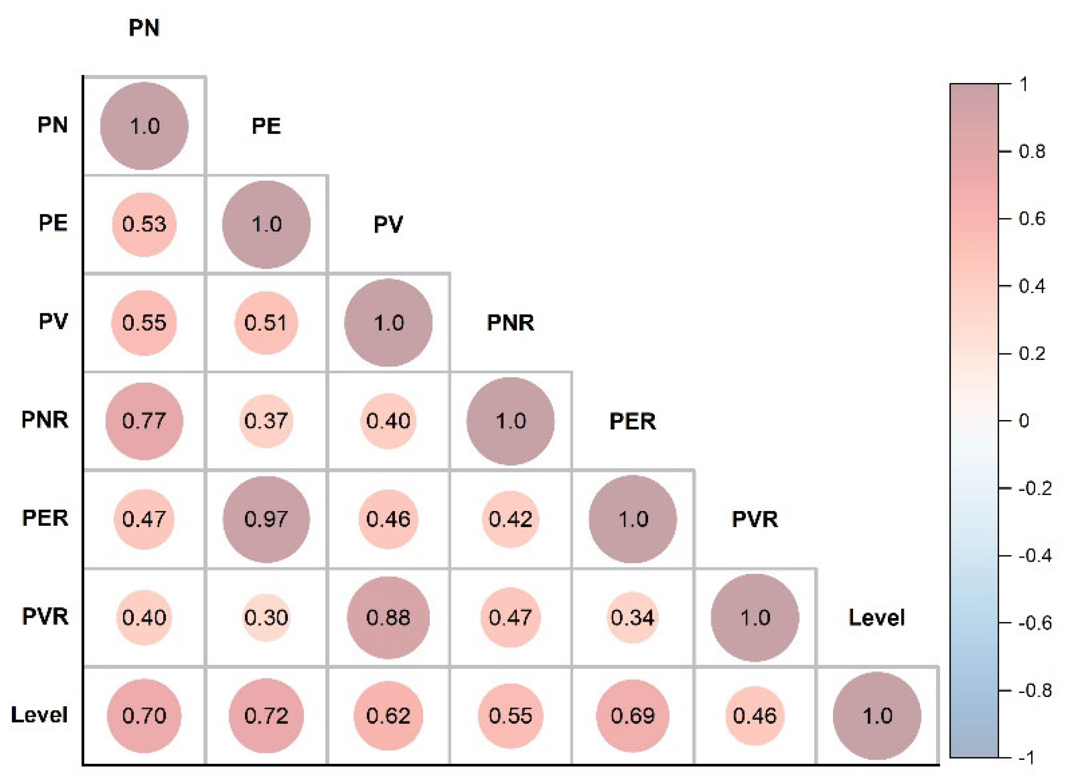
The computed correlation for the given dataset is shown in a correlation-matrix plot in Figure 5. From Figure 5, it can be seen that all indicators positively correlate with intensity levels to different extents. Four indices, PN, PE, PV, and PER, strongly correlate with targets, having correlation values above 60%, whereas PNR and PVR are moderately correlated at only 55% and 46%, respectively. In addition, some predictor-variable pairs are also strongly correlated with each other. For instance, the correlation of PE and PER is 97%, and PV and PVR follow with a correlation of 88%. Similarly, a correlation of 77% can be seen for PN and PNR. As a correlation between predictor variables becomes stronger, the redundancy of information increases and may impact the training process and prediction. Therefore, a good combination of variables should have features highly correlated with the target, yet uncorrelated with each other [31].

Depending upon the correlation analysis, a highly correlated variable can be dropped to reduce the multi-collinearity of the analysis [32]. When two variables possess a high degree of association, one can be predicted from the other. However, determining which should be removed is complicated, as the indicators selected define the rockburst based on two aspects: microfracture characteristics (PN, PE, PV) and temporal evolution characteristics (PNR, PER, PVR). Hence, if all features are dropped from either of these categories, information regarding that aspect will be lost. As a result, considering the negative consequences of one-sided feature removal, the data are further handled by implementing the dimensional-reduction technique to retain original information in low dimensions.

3.2. Dimensional Reduced Data

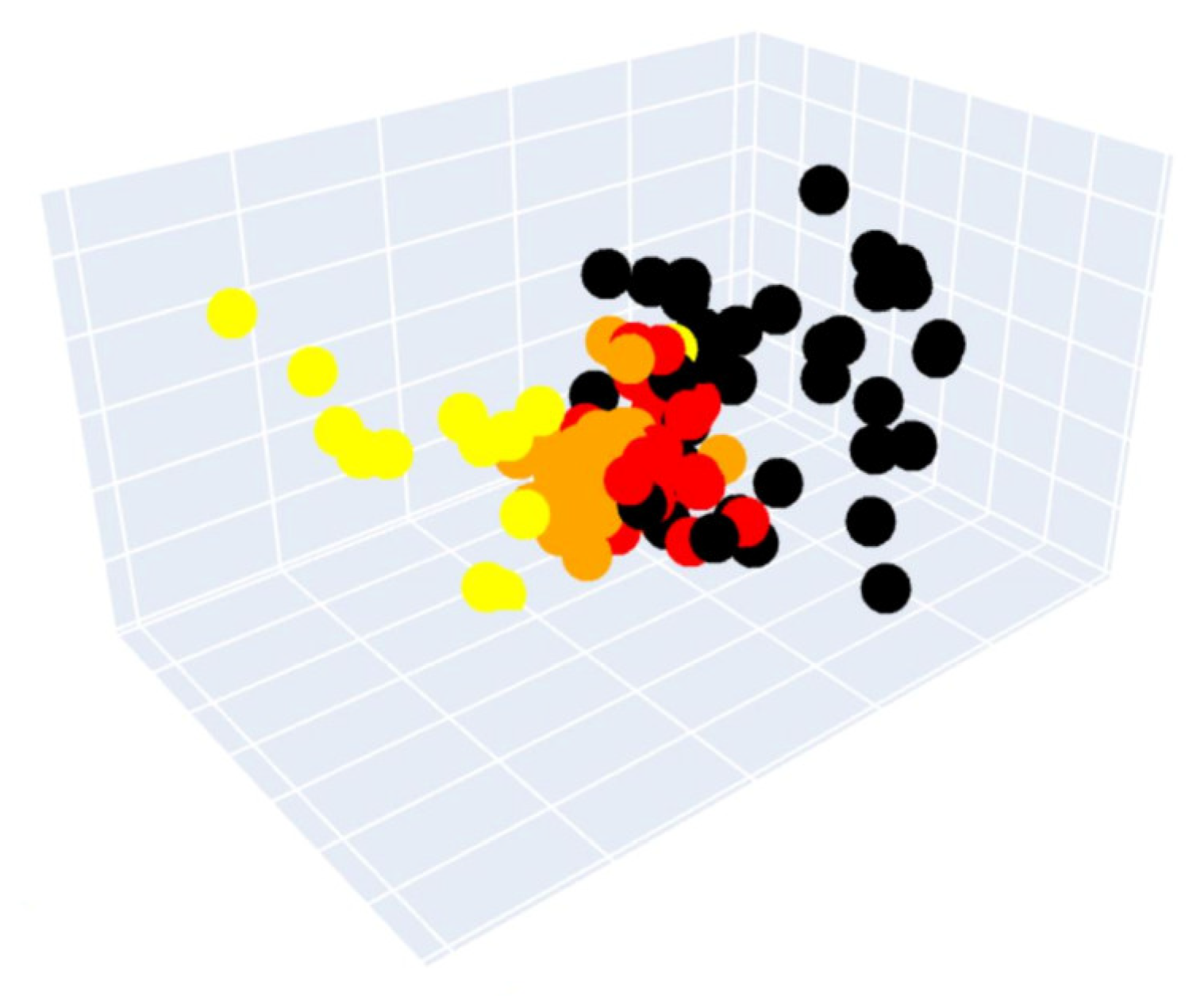
PCA was used to approach the correlated variables discussed here. PCA was implemented using the Sklearn module [33] to reduce the impact of high correlation, and the first three components to achieve the cumulative contribution rate above 80% were chosen. The individual contribution rates for the first components are 60.41%, 19.00%, and 14.82%, respectively, with a cumulative contribution rate of 94.26%. The shape of the data in the 3D space is pictured in Figure 6. It can be seen that, after scaling and PCA, the data points for each cluster are not scattered and are close to each other. The four different colours indicate the different intensity levels.

3.3. Model Training and Hyper-Parameter Optimisation

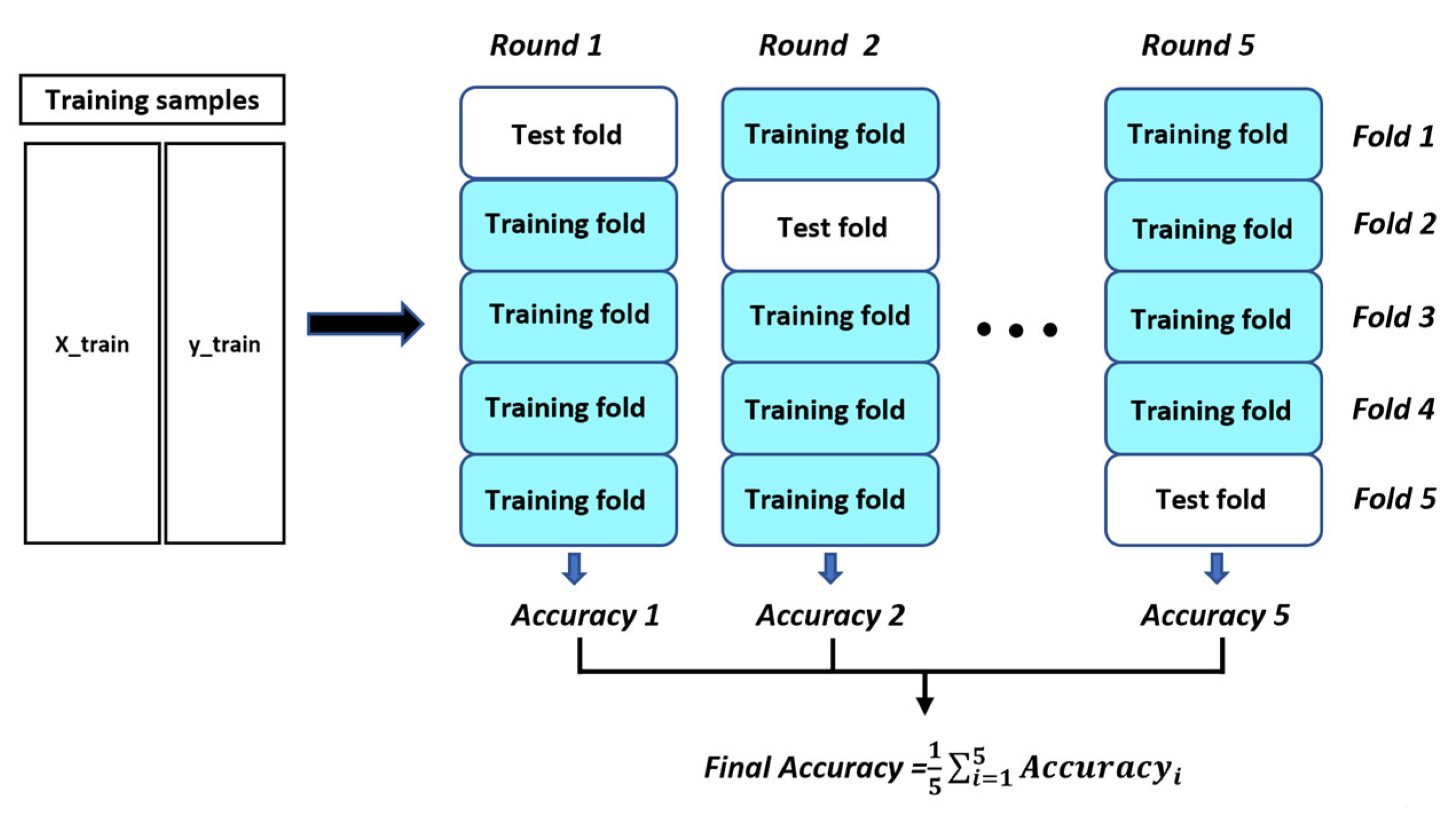
The dataset remaining after pre-processing was used to create the predictive model. The training and testing set is formed by randomly splitting the dataset into two parts, generally in an 80:20 ratio. The larger portion (79 samples) was used as the training set and was fed to the model to train it. The remaining 20 samples were used as a testing set to evaluate the model. While training the model, hyper-parameter tuning was essential and significantly increased performance. Therefore, hyper-parameters were tuned using a grid-search method that embeds the cross-validation (CV) method. The general architecture of cross-validation with five folds is portrayed in Figure 7.

Five-fold CV starts with partitioning the training dataset into five portions and training the model five times. In each round, four portions of the data act as a training set, while the remaining one acts as a test set. The results obtained from all five rounds are then averaged to obtain the final prediction [34].

To build a simple and easy-to-use model, two important hyper-parameters, depth and n_estimators, were chosen, and optimal values for each were identified. The depth is the maximum depth of the tree, and n_estimators is the total number of trees in the forest. Hyper-parameter tuning is computationally expensive. Therefore, considering the computational cost during hyper-parameter selection, values between 2 and 15 were chosen using the range function in Python to select the appropriate value for depth. Likewise, the same range function was also applied for n_estimators, and a range between 10 and 200 was specified with an interval of 10. As for the learning rate, the default setting was used.

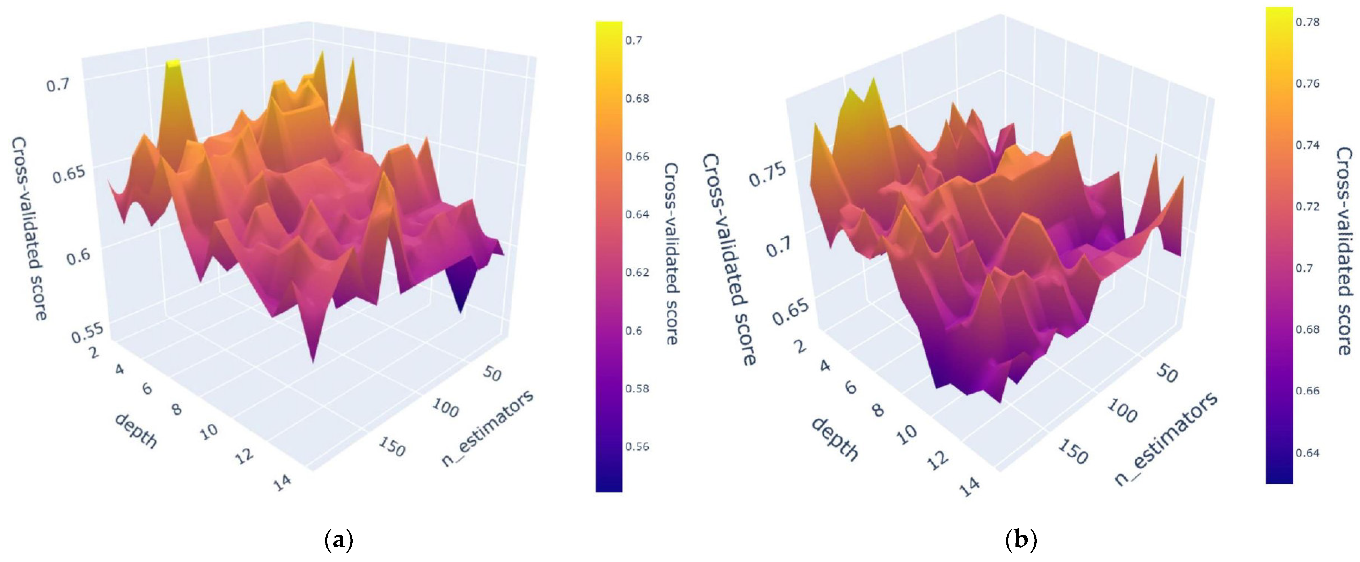
To optimise the hyper-parameters, the grid-search CV (GS-CV) method using stratified k-fold CV was adopted. This method divides the dataset into k segments such that each segment contains approximately the same percentage of samples of each target class as the complete set does. This approach is beneficial when target classes are unbalanced because it ensures that the model does not overfit to the majority class and that it is able to learn to accurately predict the minority class. GS-CV tunes the parameters by methodically building and evaluating a model for each combination of algorithm parameters, as specified in a grid [35]. Estimator and param grid are two key terms involved in using GS-CV. The estimator is a classifier that is being trained. The param grid indicates the list of parameter settings specified above. Every parameter combination is validated to seek the best accuracy, and of the possible combinations of pairs and parameter values, those that are closer to optimum are selected to yield a more precise model. The hyper-parameter optimisation results for the PCA-CGB and single CGB model that was trained on the original data are shown in Figure 8 respectively.

In Figure 7, the different colours inside the plot indicate the average accuracy for various combinations, and the taller the peak, the higher the accuracy. As illustrated, the accuracy varies significantly for different pairs of combinations. The hyper-parameter tuning range and the optimal values obtained after optimisation for PCA-CGB and CGB are given in

Table 4. Hyper-parameters and tuning range.

Classifier	Hyperparameters	Parameter Range	Interval	Optimal Value
PCA-CGB	depth	(2, 15)		3
	n_estimators	(10, 200)	10	140
CGB	depth	(2, 15)		2
	n_estimators	(10, 200)	10	130

. The optimal values acquired through the GS-CV optimisation process differ between classifiers. For PCA-CGB, the optimal depth and n_estimators are 3 and 140, respectively. Similarly, CGB has a depth value of 2 and an n_estimators value of 130.

After the best hyper-parameters were derived using GS-CV optimisation, the optimal models were used to predict the test set that was initially separated from the rest of the data and that had not been used during the training process. The confusion matrix in

Table 5. Confusion matrix for PCA-CGB and CG.

Predicted
		PCA-CGB					CGB
		0	1	2	3		0	1	2	3
True	0	9	0	1	0		8	2	0	0
	1	0	2	1	0		0	2	1	0
	2	0	0	5	0		1	1	3	0
	3	0	0	0	2		0	0	0	2

shows that, among 20 observations, the PCA-CGB predicted 18 cases correctly, only misidentifying two samples. The single CGB, by contrast has five incorrect predictions. Considering the available dataset size, the PCA-CGB has a better accuracy, at 90%. However, accuracy alone cannot reflect the overall strength of the model when the dataset has an unequally distributed class. Therefore, their strength is determined by analysing precision and recall for each class and computing the F1 score.

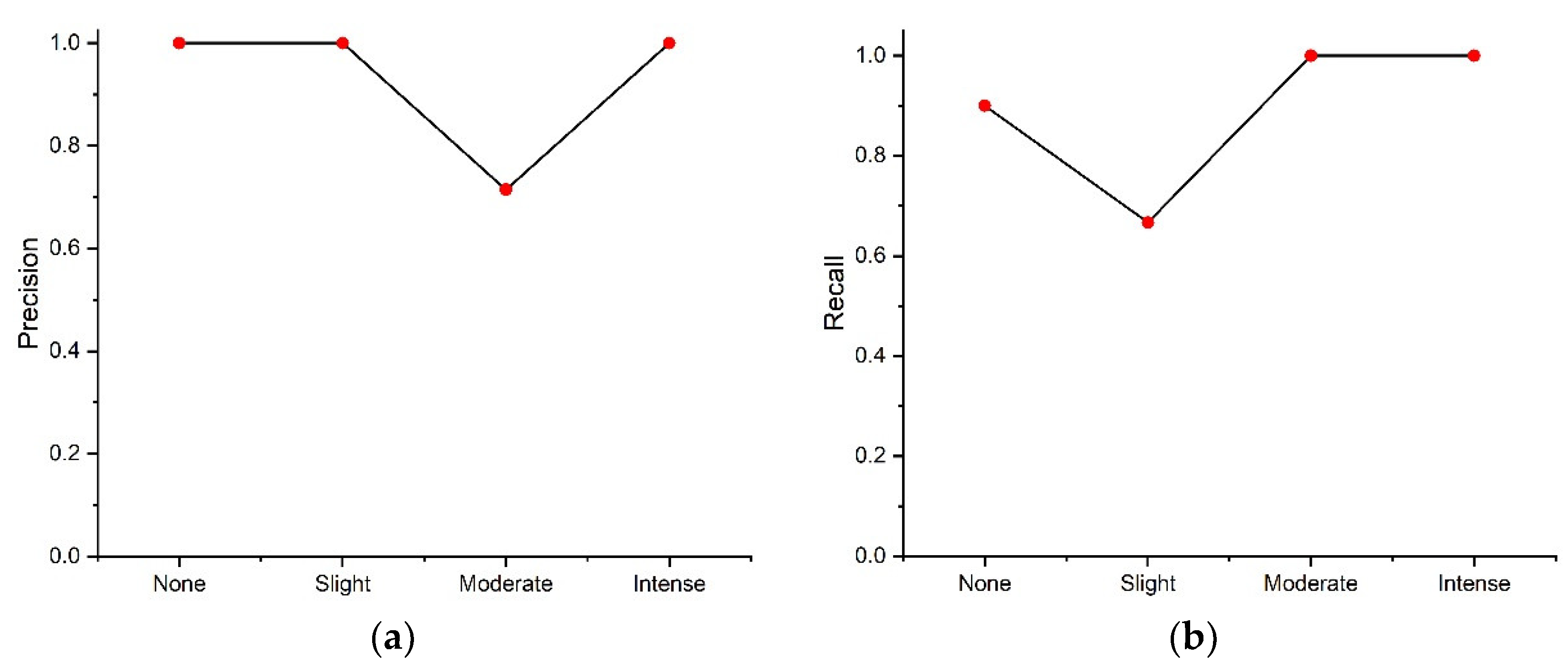
Depending on the requirements, some sectors prefer high-recall models and some sectors demand high-precision models. However, the prediction of rockburst hazards is very sensitive and focuses on two primary aspects: minimising unnecessary controlling costs and the safety of personnel and the project. If moderate and intense rockbursts are treated as high-risk and none and slight are treated as low-risk, then a model should precisely classify high-risk and low-risk cases. This should be prioritised because classifying high-risk cases as low-risk threatens human life and project safety; similarly, classifying low-risk cases as high-risk increases economic losses to control and support measures even though the high-risk event is unlikely. From this logic, it can be concluded that rockburst-hazard risk prediction is vital in accurately identifying low-risk and high-risk cases because it is equally important to minimise costs and to ensure the safety of human life and projects. Therefore, in rockburst prediction, precision and recall have equal importance. The precision and recall for the proposed work at each intensity grade are illustrated in Figure 9.

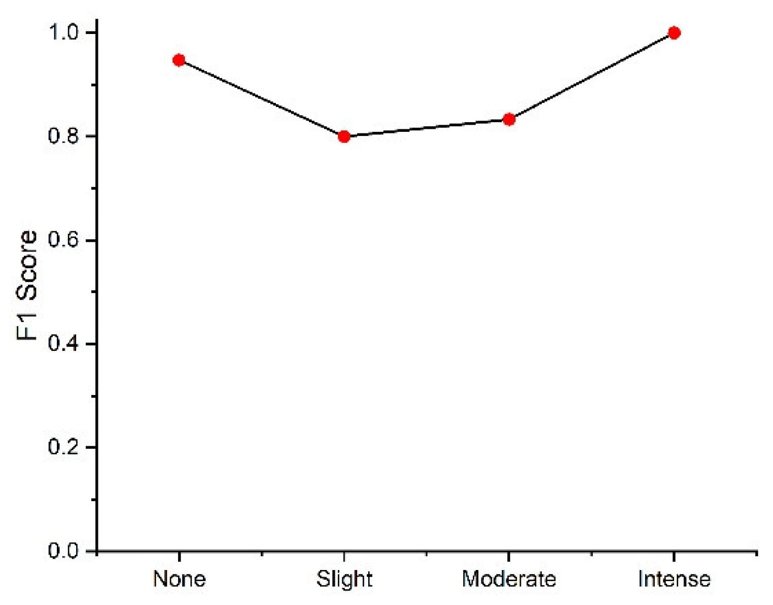
As shown in Figure 9a, PCA-CGB has high precision for none, slight, and intense rockbursts, but the precision is slightly lower for moderate rockbursts. Regarding the recall score, the values for none, moderate, and intense are greatest, whereas that for slight risk is comparatively low (Figure 8b). Overall, the model achieved precision and recall of 0.9286 and 0.8917, respectively. For any optimal model, higher precision and recall are desirable, but practically, it is difficult to maintain high precision and recall simultaneously because there is a trade-off; when one increases, another decreases. As shown in Figure 9, recall decreases when precision increases and vice versa. Hence, the F1 score determines the classifier’s strength using the harmonic mean of precision and recall. The F1 score for a single class is derived in the chart in Figure 10, and

Table 6. Description of model performance based on F1 score. Created by author based on https://stephenallwright.com/good-f1-score/ (accessed on 11 August 2023).

F1 Score	Performance Measure
Above 0.9	Very good
0.8–0.9	Good
0.5–0.8	Ok
Below 0.5	Not good

describes the general rule of thumb for determining classifier strength according to the F1 score (https://stephenallwright.com/good-f1-score/, accessed on 11 August 2023). The bar chart shows that, overall, PCA-CGB has the best F1 score for the none and intense levels, with a slightly lower score for the slight and moderate levels. It had an F1 score of 0.8952, which is considered to indicate a good classifier, according to Table 6.

4. Performance Comparison

To check the feasibility of using the PCA-CGB, its performance was compared with those of three conventional boosting classifiers on the same dataset. These other classifiers have often been utilised in rockburst prediction [17,36], and the comparison checked for improvements. The three boosting classifiers were the gradient boosting classifier (GBC) [37], adaptive boosting (AdaBoost) [38], and light gradient boosting machine (LGBM) [39]. All three models were trained on the same data after PCA, and their hyper-parameters were also optimised using the GS-CV method with the same process used for PCA-CGB. For GBC and LGBM, two crucial parameters, max_depth and n_estimators, were adopted with the same tuning range as that used for PCA-CGB. However, the parameters used for AdaBoost were slightly different; therefore, n_estimators and learning_rate were selected. The selected hyper-parameter range and obtained values are shown in

Table 7. Parameter selection for GBC, AdaBoost and HGBT.

Classifier	Hyperparameters	Parameter Range	Interval	Optimal Value
GBC	max_depth	(2, 15)		5
	n_estimators	(10, 200)	10	30
Adaboost	learning_rate	0.1–1, 0.001, 0.01, 0.005, 0.03		0.6
	n_estimators	(10, 200)	10	130
LGBM	max_depth	(2, 15)		2
	n_estimators	(10, 200)	10	100

.

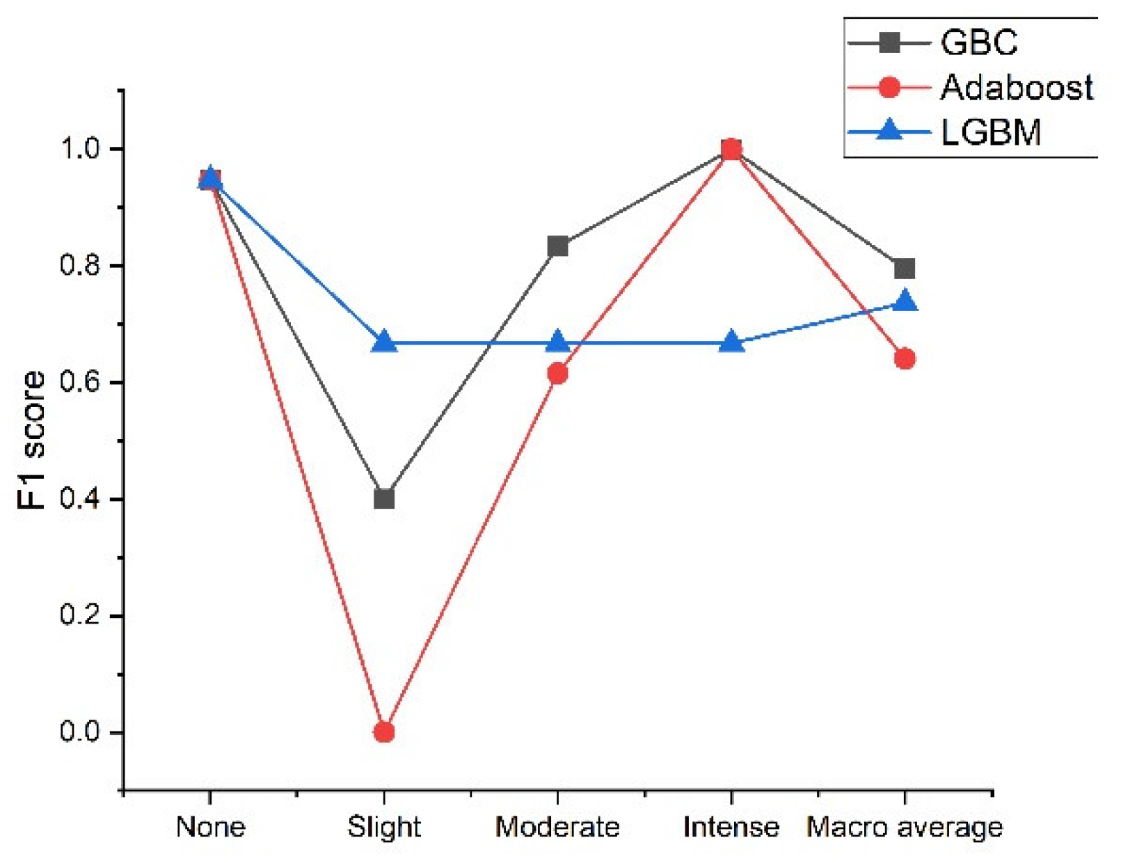
Once the optimal hyper-parameters were tuned, classifiers with optimal hyper-parameters were employed to predict the previously unseen test samples.

Table 8. Confusion matrices for GBC, AdaBoost, and LGBM.

Predicted
		GBC					AdaBoost					LGBM
		0	1	2	3		0	1	2	3		0	1	2	3
True	0	9	1	0	0		9	0	1	0		9	0	1	0
	1	0	1	2	0		0	0	3	0		0	2	1	0
	2	0	0	5	0		0	1	4	0		0	1	4	0
	3	0	0	0	2		0	0	0	2		0	0	1	1

shows the confusion matrices for GBC, AdaBoost, and LGBM. Among the three classifiers, GBC and LGBM show better results than AdaBoost. GBC misclassified one none as slight risk and two slight risks as moderate risk, whereas LGBM and AdaBoost incorrectly classified some other intensity classes as moderate risk. The F1 scores of the three classifiers are shown in Figure 11. The figure indicates that all classifiers yield better results for none/no risk and intense risk; however, all have very low scores for slight and moderate risk. GBC, AdaBoost, and LGBM generated F1 scores of 0.7952, 0.6407, and 0.7368, respectively.

Finally, the results of PCA-CGB were compared with those of these three classifiers. In various ways, the predictive performance of the proposed work is better than those of other traditional boosting classifiers when used for imbalanced rockburst data. Although GBC, AdaBoost, and LGBM seem reasonably accurate, their F1 scores are relatively low, meaning they are less robust to the above problem of class imbalance. However, the overall performance of PCA-CGB is superior concerning precision, recall, and F1 score measure, indicating that it is more reliable and possesses greater predictive power than the other boosting classifiers.

Further, in terms of F1 scores, we can discuss the performance in relation to previous work on the subject, including [18,22,40], which acquired F1 scores of 0.66, 0.8779, and 0.8631, respectively. However, the results are not directly comparable due to differences in the dataset sizes because samples for training and variables that appear in the different studies vary marginally. However, to make class distribution more diverse in this study, more cases were gathered to expand the dataset size, and a larger dataset was used compared to those in other studies. When the data are more complex, feeding a lower quantity of data for training may cause an underfitting problem, and the model loses generalisation. Therefore, more samples were used during training to ensure the model obtained enough records to learn the pattern between inputs and output. Overall, the final result for the previously unseen test set reveals that in unequally distributed data, the F1 score of the proposed approach still yields better results for all types of risk severity compared to other works, which have a low error rate even for the datasets that are mostly complex and consist of relatively few data points for particular class.

5. Field Data Validation

After the model’s reliability in prediction was verified, the model was employed to predict new engineering data extracted from [24]. The data were obtained from the underground hydropower tunnelling project after the MS activities of rockbursts were examined. After transformation using PCA, this dataset is provided as input to the model. The prediction and actual results are shown in

Table 9. Prediction of events in a new sample by PCA-CGB.

S. N	PN	PE	PV	PNR	PER	PVR	Actual	Predicted
1.	7	5.269	4.817	0.7	4.269	3.817	1	1
2.	9	1.723	4.993	1.28	0.877	4.147	1	1
3.	23	4.408	4.873	2.556	3.454	3.918	2	2

. Cases include a slight rockburst and a moderate rockburst, and the model also predicted the correct level, confirming that this classifier effectively classifies events from new, previously unseen samples.

6. Discussion and Limitations

Prediction of rockbursts in underground engineering using intelligent models should focus on correctly classifying each class equally. Generally, classical ML methods assume that all classes are equally distributed. However, when a dataset has a problem of class imbalance, relying on a single accuracy measure could be misleading because the model may correctly classify members of the majority class but fail to identify members of the minority class. In this scenario, relying on a single measure of accuracy may not be entirely reliable. For the purposes of controlling economic losses and promoting safety, the prediction of each intensity class is equally important. Section 3.3 shows that the model is highly accurate for the majority class (none/no risk) and minority class (intense risk). However, there are some inaccurate outcomes for two other minority classes, slight risk and moderate risk. If we rely on accuracy alone, the model may seem highly accurate. However, the model may fail to classify other minority classes equally, and the misclassification of these types of low-risk events as high-risk rockburst events could have serious implications. Most previous approaches that used classical ML methods relied on a single accuracy measure to evaluate the classifier’s performance. Rather than depending on a single metric, this study used precision, recall, and F1 scores because they indicate how robust the classifier is when applied to imbalanced classes. If the model’s performance is compared using the F1 score, it is reasonable and acceptable to suggest that it is not susceptible to performance problems associated with imbalanced cases and has greater power to distinguish among classes. The model’s performance can also be confirmed when it is applied to rockburst classes that constitute a less extreme minority, as it can accurately identify events in such classes. Nevertheless, the model yields a slightly lower F1 score for slight and moderate rockbursts, the primary reason for which might be uncertainties and overlap between the two cases, which in turn might have led to misclassifications. Despite this issue, PCA-CGB is still more powerful than traditional boosting classifiers because while they seem accurate, they have lower scores in other metrics, indicating that their performance in predicting rockburst data is weak.

Although the proposed method yielded satisfactory results, the dataset size is still relatively small compared to those seen in common ML tasks. In common practice, ML methods rely heavily on huge datasets for better generalisation. Very small datasets can significantly lower performance by underfitting or overfitting the model. Thus, future research should focus on enhancing the model’s robustness by developing a model from larger datasets.

7. Conclusions

Predicting short-term rockburst risk accurately has always been important, as it directly threatens the safety of personnel, equipment, and subsurface structures. Equally, classifying risk severity is essential to allowing the adoption of efficient control measures to avoid economic loss and ensure personnel safety. However, reliably distinguishing among risk levels is often challenging due to class-imbalance issues. Most existing work relies on models with high accuracy, but some of them cannot perform well with imbalanced data. Hence, this work proposes a simple, intelligent predictive method combining unsupervised learning, principal component analysis (PCA), and supervised categorical gradient-boosting (CGB) approaches to intelligently predict rockburst risk levels. The value of this method is that it can generate predictions on unequally distributed classes more efficiently than classical ML models can. The real engineering data based on microseismic information were as assembled into a supportive database comprising six features. The variables have high correlation; therefore, PCA reduces redundancy among variables. After reducing the original dimension into three components, the CGB is adopted to create a PCA-CGB model to predict rockburst risk. To ensure that the optimal model is produced, hyper-parameters are tuned to obtain the best output. The model’s predictive performance was evaluated using precision, recall, and F1 score and further compared with three traditional boosting techniques to check for feasibility. The results showed that, regarding multiple performance measures, CGB with PCA data surpassed all conventional techniques and achieved precision, recall, and F1 scores of 0.9286, 0.8917, and 0.8952, respectively. In particular, when dataset have higher degree of correlation and classes are unevenly distributed, the output of PCA-CGB is more stable and effectively identifies majority and minority classes at higher rates than do the conventional methods. The final model also predicts new cases collected from the underground engineering project, accurately matching the corresponding actual events. The proposed work supports the management of rockburst risk because it can categorise and classify various risk levels with a degree of accuracy.

References

1. Heal, D. Observations and Analysis of Incidences of Rockburst Damage in Underground Mines; University of Western Australia: Crawley, Australia, 2010. [Google Scholar]
2. Liu, F.; Ma, T.; Chen, F. Prediction of rockburst in tunnels at the Jinping II hydropower station using microseismic monitoring technique. Tunn. Undergr. Space Technol. 2018, 81, 480–493. [Google Scholar] [CrossRef]
3. Bruning, T.D. A Combined Experimental and Theoretical Investigation of the Damage Process in Hard Rock with Application to Rockburst; University of Adelaide: Adelaide, Australia, 2018. [Google Scholar]
4. Ortlepp, W. RaSiM comes of age—A review of the contribution to the understanding and control of mine rockbursts. In Proceedings of the Sixth International Symposium on Rockburst and Seismicity in Mines, Perth, Australia, 10–14 September 2005; pp. 9–11. [Google Scholar]
5. Hong, K.; Zhou, D. Rockburst characteristics and control measures in Taipingyi tunnels. Chin. J. Rock Mech. Eng. 1995, 14, 171–178. [Google Scholar]
6. Liu, J.; Feng, X.; Li, Y.; Xu, S.; Sheng, Y. Studies on temporal and spatial variation of microseismic activities in a deep metal mine. Int. J. Rock Mech. Min. Sci. 2013, 60, 171–179. [Google Scholar] [CrossRef]
7. Ortlepp, W.D.; Stacey, T.R. Rockburst mechanisms in tunnels and shafts. Tunn. Undergr. Space Technol. 1994, 9, 59–65. [Google Scholar] [CrossRef]
8. He, H.; Dou, L.; Gong, S.; He, J.; Zheng, Y.; Zhang, X. Microseismic and electromagnetic coupling method for coal bump risk assessment based on dynamic static energy principles. Saf. Sci. 2019, 114, 30–39. [Google Scholar] [CrossRef]
9. Li, N.; Huang, B.; Zhang, X.; Yuyang, T.; Li, B. Characteristics of microseismic waveforms induced by hydraulic fracturing in coal seam for coal rock dynamic disasters prevention. Saf. Sci. 2019, 115, 188–198. [Google Scholar] [CrossRef]
10. Feng, G.L.; Feng, X.T.; Chen, B.R.; Xiao, Y.X.; Yu, Y. A Microseismic Method for Dynamic Warning of Rockburst Development Processes in Tunnels. Rock Mech. Rock Eng. 2015, 48, 2061–2076. [Google Scholar] [CrossRef]
11. Feng, X.; Yu, Y.; Feng, G.; Xiao, Y.; Chen, B.; Jiang, Q. Fractal behaviour of the microseismic energy associated with immediate rockbursts in deep, hard rock tunnels. Tunn. Undergr. Space Technol. 2016, 51, 98–107. [Google Scholar] [CrossRef]
12. Mendecki, A. Seismic Monitoring in Mines; Springer: Berlin/Heidelberg, Germany, 1997. [Google Scholar]
13. Yu, Y.; Geng, D.; Tong, L.; Zhao, X.; Diao, X.; Huang, L. Time Fractal Behavior of Microseismic Events for Different Intensities of Immediate Rock Bursts. Int. J. Geomech. 2018, 18, 06018016. [Google Scholar] [CrossRef]
14. Chen, B.; Feng, X.; Li, Q.; Luo, R.; Li, S. Rock Burst Intensity Classification Based on the Radiated Energy with Damage Intensity at Jinping II Hydropower Station, China. Rock Mech. Rock Eng. 2015, 48, 289–303. [Google Scholar] [CrossRef]
15. Alcott, J.M.; Kaiser, P.K.; Simser, B.P. Use of Microseismic Source Parameters for Rockburst Hazard Assessment. Pure Appl. Geophys. 1998, 153, 41–65. [Google Scholar] [CrossRef]
16. Feng, G.; Xia, G.; Chen, B.; Xiao, Y.; Zhou, R. A Method for Rockburst Prediction in the Deep Tunnels of Hydropower Stations Based on the Monitored Microseismicity and an Optimized Probabilistic Neural Network Model. Sustainability 2019, 11, 3212. [Google Scholar] [CrossRef]
17. Liang, W.; Sari, A.; Zhao, G.; McKinnon, S.D.; Wu, H. Short-term rockburst risk prediction using ensemble learning methods. Nat. Hazards 2020, 104, 1923–1946. [Google Scholar] [CrossRef]
18. Liang, W.; Sari, Y.A.; Zhao, G.; McKinnon, S.D.; Wu, H. Probability Estimates of Short-Term Rockburst Risk with Ensemble Classifiers. Rock Mech. Rock Eng. 2021, 54, 1799–1814. [Google Scholar] [CrossRef]
19. Liu, G.; Jiang, Q.; Feng, G.; Chen, D.; Chen, B.; Zhao, Z. Microseismicity-based method for the dynamic estimation of the potential rockburst scale during tunnel excavation. Bull. Eng. Geol. Environ. 2021, 80, 3605–3628. [Google Scholar] [CrossRef]
20. Zhao, H.; Chen, B.; Zhu, C. Decision Tree Model for Rockburst Prediction Based on Microseismic Monitoring. Adv. Civ. Eng. 2021, 2021, 8818052. [Google Scholar] [CrossRef]
21. Toksanbayev, N.; Adoko, A. Predicting rockburst damage scale in seismically active mines using a classifier ensemble approach. IOP Conf. Ser. Earth Environ. Sci. 2023, 1124, 012102. [Google Scholar] [CrossRef]
22. Ullah, B.; Kamran, M.; Yichao, R. Predictive Modeling of Short-Term Rockburst for the Stability of Subsurface Structures Using Machine Learning Approaches: T-SNE, K-Means Clustering and XGBoost. Mathematics 2022, 10, 449. [Google Scholar] [CrossRef]
23. Tanha, J.; Abdi, Y.; Samadi, N.; Razzaghi, N.; Asadpour, M. Boosting methods for multi-class imbalanced data classification: An experimental review. J. Big Data 2020, 7, 70. [Google Scholar] [CrossRef]
24. Feng, X.; Chen, B.; Zhang, C.; Li, S.; Wu, S. Mechanism, Warning and Dynamic Control of Rockburst Development Process; Science Press Beijing: Beijing, China, 2013. [Google Scholar]
25. Mohamed Salleh, F.H.; Arif, S.M.; Zainudin, S.; Firdaus-Raih, M. Reconstructing gene regulatory networks from knock-out data using Gaussian Noise Model and Pearson Correlation Coefficient. Comput. Biol. Chem. 2015, 59 Pt B, 3–14. [Google Scholar] [CrossRef]
26. Yin, X.; Liu, Q.; Pan, Y.; Huang, X.; Wu, J.; Wang, X. Strength of Stacking Technique of Ensemble Learning in Rockburst Prediction with Imbalanced Data: Comparison of Eight Single and Ensemble Models. Nat. Resour. Res. 2021, 30, 1795–1815. [Google Scholar] [CrossRef]
27. Prokhorenkova, L.; Gusev, G.; Vorobev, A.; Dorogush, A.V.; Gulin, A. CatBoost: Unbiased boosting with categorical features. In Proceedings of the 32nd Conference on Neural Information Processing Systems (NeurIPS 2018), Montréal, QC, Canada, 3–8 December 2018. [Google Scholar]
28. Wu, T.; Zhang, W.; Jiao, X.; Guo, W.; Hamoud, Y.A. Comparison of five Boosting-based models for estimating daily reference evapotranspiration with limited meteorological variables. PLoS ONE 2020, 15, e0235324. [Google Scholar] [CrossRef] [PubMed]
29. Shahani, N.M.; Kamran, M.; Zheng, X.; Liu, C.; Guo, X. Application of Gradient Boosting Machine Learning Algorithms to Predict Uniaxial Compressive Strength of Soft Sedimentary Rocks at Thar Coalfield. Adv. Civ. Eng. 2021, 2021, 2565488. [Google Scholar] [CrossRef]
30. Goutte, C.; Gaussier, É. A Probabilistic Interpretation of Precision, Recall and F-Score, with Implication for Evaluation. In Proceedings of the European Conference on Information Retrieval, Santiago de Compostela, Spain, 21–23 March 2005. [Google Scholar]
31. Hall, M.A. Correlation-Based Feature Selection for Machine Learning. Ph.D. Thesis, The University of Waikato, Hamilton, New Zealand, 1999. [Google Scholar]
32. Midi, H.; Sarkar, S.K.; Rana, S. Collinearity diagnostics of binary logistic regression model. J. Interdiscip. Math. 2010, 13, 253–267. [Google Scholar] [CrossRef]
33. Pedregosa, F.; Varoquaux, G.; Gramfort, A.; Michel, V.; Thirion, B.; Grisel, O.; Blondel, M.; Prettenhofer, P.; Weiss, R.; Dubourg, V.; et al. Scikit-learn: Machine Learning in Python. J. Mach. Learn. Res. 2012, 12, 2825–2830. [Google Scholar]
34. Liu, L.; Zhao, G.; Liang, W. Slope Stability Prediction Using k-NN-Based Optimum-Path Forest Approach. Mathematics 2023, 11, 3071. [Google Scholar] [CrossRef]
35. Ranjan, G.S.K.; Verma, A.K.; Radhika, S. K-Nearest Neighbors and Grid Search CV Based Real Time Fault Monitoring System for Industries. In Proceedings of the 2019 IEEE 5th International Conference for Convergence in Technology (I2CT), Pune, India, 29–31 March 2019; pp. 1–5. [Google Scholar]
36. Ge, Q.; Feng, X. Classification and prediction of rockburst using AdaBoost combination learning method. Rock Soil Mech. 2008, 29, 943–948. [Google Scholar]
37. Aler, R.; Galván, I.M.; Ruiz-Arias, J.A.; Gueymard, C.A. Improving the separation of direct and diffuse solar radiation components using machine learning by gradient boosting. Sol. Energy 2017, 150, 558–569. [Google Scholar] [CrossRef]
38. Freund, Y.; Schapire, R.E. A Decision-Theoretic Generalization of On-Line Learning and an Application to Boosting. J. Comput. Syst. Sci. 1997, 55, 119–139. [Google Scholar] [CrossRef]
39. Ke, G.; Meng, Q.; Finley, T.; Wang, T.; Chen, W.; Ma, W.; Ye, Q.; Liu, T. LightGBM: A Highly Efficient Gradient Boosting Decision Tree. In Proceedings of the 31st Conference on Neural Information Processing Systems (NIPS 2017), Long Beach, CA, USA, 4–9 December 2017. [Google Scholar]
40. Qiu, Y.; Zhou, J. Short-term rockburst prediction in underground project: Insights from an explainable and interpretable ensemble learning model. Acta Geotech. 2023. [Google Scholar] [CrossRef]
Figure 1. Flow chart of the proposed work.
Bdcc 07 00172 g001
Figure 2. Feature variables for rockburst prediction.
Bdcc 07 00172 g002aBdcc 07 00172 g002b
Figure 3. Histograms for all six features.
Bdcc 07 00172 g003aBdcc 07 00172 g003b
Figure 5. Correlation-matrix plot for MS indicators.
Bdcc 07 00172 g005
Figure 6. Projection of data into 3D space after PCA transformation.
Bdcc 07 00172 g006
Figure 7. The working principle of five-fold cross-validation.
Bdcc 07 00172 g007
Figure 8. Visualisation plots for hyper-parameter optimisation. (a) PCA-CGB; (b) CGB.
Bdcc 07 00172 g008
Figure 9. Precision and recall for PCA-CGB. (a) Precision; (b) recall.
Bdcc 07 00172 g009
Figure 10. F1 score for PCA-CGB.
Bdcc 07 00172 g010
Figure 11. F1 scores for GBC, AdaBoost, and LGBM.
Bdcc 07 00172 g011