Article

Semi-Supervised Classification with A*: A Case Study on Electronic Invoicing

by
Bernardo Panichi
and
Alessandro Lazzeri
*
Polaris Engineering Spa, Via Turati 29, 20121 Milano, Italy
*
Author to whom correspondence should be addressed.
Big Data Cogn. Comput. 2023, 7(3), 155; https://doi.org/10.3390/bdcc7030155
Submission received: 17 July 2023 / Revised: 14 September 2023 / Accepted: 18 September 2023 / Published: 20 September 2023
(This article belongs to the Special Issue Computational Finance and Big Data Analytics)

Abstract

:
This paper addresses the time-intensive task of assigning accurate account labels to invoice entries within corporate bookkeeping. Despite the advent of electronic invoicing, many software solutions still rely on rule-based approaches that fail to address the multifaceted nature of this challenge. While machine learning holds promise for such repetitive tasks, the presence of low-quality training data often poses a hurdle. Frequently, labels pertain to invoice rows at a group level rather than an individual level, leading to the exclusion of numerous records during preprocessing. To enhance the efficiency of an invoice entry classifier within a semi-supervised context, this study proposes an innovative approach that combines the classifier with the A* graph search algorithm. Through experimentation across various classifiers, the results consistently demonstrated a noteworthy increase in accuracy, ranging between 1% and 4%. This improvement is primarily attributed to a marked reduction in the discard rate of data, which decreased from 39% to 14%. This paper contributes to the literature by presenting a method that leverages the synergy of a classifier and A* graph search to overcome challenges posed by limited and group-level label information in the realm of electronic invoicing classification.

1. Introduction

Corporate accounting represents an area replete with numerous repetitive and highly automatable tasks, offering a fertile ground for the integration of artificial intelligence to support accounting professionals. As a matter of fact, the role of accountants is widely acknowledged as being among the most susceptible to computerization, as substantiated by a research paper [1]. In this landscape of evolving technology, our study delves into a critical facet of corporate accounting: the classification of invoice entries [2,3]. By employing innovative machine learning techniques, we aim to alleviate the burden of manual work, streamline processes, and improve overall efficiency in the realm of electronic invoicing.
Electronic invoicing, often referred to as e-invoicing, has arisen as a contemporary, dependable, and efficient approach for managing and processing invoices related to products, services, taxes, and various goods, eliminating the requirement for physical paper documents [4]. E-invoicing presents a range of compelling advantages. Firstly, it expedites transaction processes, leading to faster delivery times, shorter payment delays, and a notable reduction in human errors. Secondly, e-invoicing holds the promise of automation, particularly when a structured format is employed, streamlining the generation and seamless transfer of invoices throughout the supply chain. Additionally, it brings about cost efficiencies by reducing the need for printing and postage. For consumers, this digital approach enhances convenience, lowering the likelihood of forgetting payments and thereby reducing the risk of fines. Beyond these practical benefits, e-invoicing contributes to a greener environment by curbing paper consumption and reducing energy costs associated with the physical transportation of invoices from one location to another [5]. These benefits have prompted policymakers worldwide to enact legislation aimed at incentivizing firms to adopt this innovative technology [3].
However, it is important to note that even in this electronic landscape, significant manual work persists [2]. This persistence is attributed to several key challenges:
  • Categorization Complexity: At the heart of electronic invoicing is the categorization of invoice entries within the general book. Each entry must adhere to a specific system of categories, offering a high degree of flexibility. Individual firms often customize these categories to meet their unique needs. Consequently, the same invoice entry may yield different categorizations across different firms. Additionally, one issuer may provide multiple services or products with distinct invoice reasons, making automatic categorization a non-trivial task [6].
  • Evolving Accounting Legislation: Another layer of complexity arises from the continuously evolving accounting regulations designed to adapt to the dynamic economy. These changes can significantly impact the logic and procedures involved in the invoicing process, necessitating adaptive solutions [4].
  • Rule-Based Systems: To address these complexities, many software programs have introduced rule-based systems. While effective in simple scenarios, these systems struggle to maintain the vast array of rules required to handle complex and varied situations [7].
The challenges outlined here underscore the need for innovative solutions that can adapt to evolving regulations, handle diverse categorization scenarios, and alleviate the persistent burden of manual work on bookkeepers.
Electronic invoicing classification poses a significant challenge in the field of artificial intelligence, attracting the attention of researchers and practitioners alike [8]. Prior efforts have grappled with the computational complexity arising from the need to construct a dataset for supervised learning that combines information from two distinct documents: electronic invoices and the account journal.
One of the fundamental challenges in this context is establishing a direct correspondence between individual invoice lines (i.e., the samples to be classified) and their corresponding accounting accounts (i.e., the target variables) [8]. This challenge arises due to the granularity of invoice lines, which provide a detailed breakdown of transactions, contrasting with the broader, hierarchical categorization found in the account journal. Importantly, the account journal lacks any inherent information about which lines are categorized in a specific account, obscuring the association between them.
As a result, a substantial volume of potentially valuable data is discarded during the dataset construction phase because of the inability to match data with their respective target labels. However, these unlabeled data carry valuable information that could significantly enhance classifier performance if utilized effectively.
To address this challenge, we adopt a semi-supervised learning approach [9], where unsupervised data are coupled with pseudo-labels. In this paper, our approach distinguishes itself by mitigating a critical limitation of semi-supervised learning—the quality of pseudo-labels—by leveraging the A* search algorithm.
More precisely, the main objectives of this study can be summarized as follows:
  • Automate the Electronic Invoicing: the primary goal is to reduce the necessity of extensive and manual intervention in the accounting process.
  • Enhance Classification Accuracy: to achieve the primary goal, we need to improve the accuracy, and reduce the missclassifications and errors of the machine learning algorithm.
  • Develop a Semi-Supervised Framework: design and implement a semi-supervised learning algorithm capable of integrating supervised and unsupervised data.
  • Overcome pseudo-label generation challenges and leverage the group-instance structure: Investigate, propose and implement methodologies that effectively generate high-quality pseudo-labels for unsupervised data using a graph search algorithm (A*).
In summary, our framework offers a systematic and comprehensive semi-supervised approach to address the intricate challenges inherent in electronic invoicing classification. Each step is meticulously designed to optimize classification accuracy and efficiency within the corporate accounting domain.
The significance of this study lies in its potential to make meaningful advancements in the field of electronic invoicing classification within corporate accounting. Despite the progress made in electronic invoicing, challenges persist in accurately categorizing individual invoice entries. Through the introduction of a robust semi-supervised learning framework, in conjunction with the precision of the A* search algorithm, this research seeks to address a persistent obstacle in the field. The study aims to improve the accuracy and efficiency of electronic invoicing classification, potentially reducing the reliance on manual processes and maximizing the utility of unsupervised data. Furthermore, this research endeavors to contribute new insights to the domain and offer practical solutions that can empower corporate accountants to navigate the complexities of electronic invoicing with greater precision and efficiency, potentially marking a significant step forward in corporate accounting practices.
After introducing the research questions and goals of our study, in Section 2 we provide an overview of the most recent and significant work in the same field, then the general problem of invoice entries classification is formalized in Section 3. In Section 4 the methodological approach mentioned above is explained step by step to show how it is useful in solving the problem to a higher level of accuracy. Later, Section 5 is devoted to a discussion of our experiments and the improvements achieved through the semi-supervised approach. Finally, Section 6 contains conclusions.

2. Literature Review

In recent years, many efforts have been made to apply intelligent artificial systems to the accounting field. There are several works aimed at providing a general overview of what are the applications and results of machine learning in accounting. In Ref. [10] the authors trace some typical tasks of an accountant’s profession in which machine learning has been successfully applied, like reviewing source documents, analyzing business transactions and assessing risks, while also dwelling on the ethical implications of this; whereas, Ref. [11] focuses mainly on the main unexplored opportunities for machine learning in accounting and Ref. [4] offers a systematic literature review in the field of e-invoicing.
Historically, the first attempts to introduce technological tools to support the accountant’s work date back to the 1990s, when the first Optical Character Recognition (OCR) systems were developed. More recently, with the advent of artificial intelligence and machine learning, major strides have been made in this area. For example, the work of Tarawneh et al. aims to recognize, by training an automatic classifier, handwritten and machine-printed invoices [12], while Ha et al. propose a system for recognizing the initial page of an invoice among a series of business documents [13]. Very recently, Li developed an automatic invoice recognition system that can accurately recognize digital information from an invoice image thanks to deep learning [14]. Recent overviews about Computer Vision applications in the accounting field are [15,16].
Also thanks to the advent of machine learning, it was possible to start making accurate estimates and predictions in accounting based on historical data. Two interesting examples are the following. In Ref. [17] the authors design a method to estimate loss reserves (future customer claims) based on insurance companies’ data, whereas an accounting fraud detection system based on an AI classifier is presented by Ref. [18].

2.1. Automatic Invoice Labeling

Since the spreading of the e-invoice, many researchers are proposing innovative machine learning frameworks to support the accountants in both invoice labeling and transaction labeling tasks. In the former, the scope is to assign a label to an invoice [12,19]. In the latter, the aim is to assign a label (code) to each line of the invoice.
Our work also fits into this family, as it proposes a system for estimating the nature of a transaction, the same objective of [6,20,21]. As the best of our knowledge, Bengtsson et al. were the first ones to deal with this specific task. In their work they present some preliminary research about using machine learning for automatic invoice labeling, but still failing to outperform traditional deterministic techniques. Later, the work from Bergdorf claims the superiority of more advanced machine learning models over fixed rule-based methods when it comes to classifying the transactions reported in an invoice according to natures. In Ref. [21] the authors compared traditional term frequency models such as TF-IDF, with Convolutions models applied to text classification. The experiments show that convolutional neural networks can manage short text sentences, even with errors and typos, better achieving an overall accuracy score of 86.9 % . Ref. [22] studied the hierarchical taxonomy of the account code and reconciled bank accounts. By leveraging this structure the authors added important features to the dataset and achieved a performance with the Top-K Parent Boosting algorithm up to 95.5 % .
The context in which we operated lends itself particularly well to continuing this line of research because in Italy it was made mandatory for all business activities since January 2019 to issue electronic invoices in standardized XML format. In fact, Bardelli et al. [8] compared several machine learning algorithms (Random Forest, AdaBoost and MultiLayer Perceptron) and preprocessing (Bag of Words and Word2Vec) techniques on a large datasets of invoices (order of 300,000 lines). The authors achieved up to 98.9 and 89.8 % f1-score on sent and received invoice respectively. Within their work, Bardelli et.al. ran into the challenge of constructing a purely supervised dataset, which led them to discard 39 % of the potentially usable data.
Our contribution in this area lies precisely in the optimization of the data of received invoices, by working in a semi-supervised framework with the aim of reducing the discarded rate, and consequently improve the accuracy of the classification models.

2.2. Semi-Supervised Learning

Semi-supervised learning occupies a conceptual middle ground between supervised and unsupervised learning, enabling the utilization of substantial volumes of unlabeled data commonly found in numerous scenarios, alongside relatively smaller sets of labeled data [9].
In the landscape of semi-supervised learning, there are two primary approaches: inductive and transductive methods [9]. In the inductive approach, the focus is on constructing an initial classification model using the labeled data, which is then applied to make predictions on the unlabeled data. Conversely, transductive methods are primarily concerned with generating label predictions specifically for the provided unlabeled data points [9].
In our research, we have consciously chosen to adopt the inductive approach. This decision aligns with our overarching goal of training a classifier that can effectively categorize electronic invoicing entries.
Notably, other researchers applied inductive semi-supervised learning on document classification tasks. For instance, Ref. [23] adopted semi-supervised learning on keywords to analyze a corpus of unstructured text documents regarding accounts receivable disputes at a large corporation. According to the authors, the semi-supervised approach reduced the manual effort of labeling time by 50 % . Similarly, Ref. [24] fine-tuned a variational autoencoder base on the BERT architecture for text classification in a semi-supervised context. The authors experimented on four benchmark dataset (AG, Hatespeech, IMDB, and Yahoo!) by simulating missing labels. According to their results, such semi-supervised learning is an efficient and effective approach to text classification when data and computation are limited. Furthermore, Ref. [25] explored the application of LSTM deep neural networks for the embeddings of text regions. Such approach, which can convey complex concepts, resulted more useful than embeddings of single words in isolation. Ref. [26] evaluated the impact of adversarial and virtual adversarial training on the regularization performance in sequence models on text classification tasks. The overall performance on benchmark dataset exceeded or was on par with the state of the art performance. Moreover, the authors identified a better quality of word embeddings.
In essence, semi-supervised learning has consistently demonstrated its effectiveness and efficiency in uncovering latent knowledge within unlabeled data, all without significantly burdening domain experts with increased labeling efforts. Thus, it serves as a well-suited learning paradigm for our research context.

2.3. Graph Search

Moreover, many recent approaches for semi-supervised learning exploit regularization techniques and encourage the model to generalize better to unseen data [27]. One of this techniques are Graph-Based Methods. Generally, the labeled and unlabeled data points can be considered as nodes of a graph, and the objective is to propagate the labels from the labeled nodes to the unlabeled ones by utilizing the similarity of two nodes, which is reflected by how strong the edge between the two nodes [28]. For instance, Ref. [29] propagated the learning sequence of unlabeled data from simple to difficult examples. More in detail, the algorithm alternates between two paradigms, teaching-to-learn and learning-to-teach (TLLT). In the teaching-to-learn step, the learner conducts the propagation on the simplest unlabeled examples designated by the teacher. In the learning-to-teach step, the teacher incorporates the learner’s feedback to adjust the choice of the subsequent simplest examples. Similarly, Ref. [30] trained a deep neural network on the supervised data. Then, they iteratively build a nearest neighbor graph of the entire training set in the feature space of the current network, and propagate the labels to the unsupervised data. Finally, the network is retrained on the entire training set. More graph-based methods can be found in Ref. [28].
Differently from previous applications, our setting allow us to leverage the hierarchical structure of the invoice and the account book. This relation permits to build a very peculiar graph that differs from the typical topology of graph based methods. More precisely, we build the graph after assigning the pseudo-labels to the invoice lines: a node is a candidate solution, i.e., a set of couples {(line, pseudo-label)}, while an edge is a modification of one of the pseudo-label. Here, the scope is to navigate the graph to find a valid solution, i.e., a solution is valid if all the pseudo-labels of the invoice lines match the account book.
As several graph search algorithms can be applied, such as random walk, deep-first or breadth-first, in Section 4.4 we discuss the structure of the graph and the condition that allow the adoption of a much efficient solution: A* graph search.

2.4. Literature Summary

The comparative Table 1 offers a quick visual summary of the research work just described, showing where our work is placed.
The first column refers to works that applied Computer Vision techniques, such as OCR; the second to researches that used Machine Learning techniques to estimate quantities of interest in accounting; the third to studies that focused on the problem of determining the nature of a transaction, the fifth to works that attempted to optimise the available data by working in a semi-supervised framework and finally, the last column, to articles that coupled it with a graph search.

3. Problem Description

As anticipated, the core goal of this work is to provide an accountant with an accurate artificial intelligence classifier capable of understanding the nature of the various transactions that make up an invoice to reduce time-consuming manual intervention in labeling them.
Table A1 in the Appendix A section introduces all the variables needed to formulate our problem. Please refer to it throughout the next paragraphs.
Before doing model selection and training, it is necessary to build a dataset containing as many invoice rows as possible with their respective codes, from which the algorithm can learn the input-output relationship.
Our starting dataset D is made up of pairs (X, S). Each invoice X i has a corresponding account journal section S i , i U (more detailed explanations on the structure of electronic invoices are provided in the Appendix B). Thus, the first challenge is about combining data from two different sources:
  • On the one hand, we have a collection of invoices X i , each one with multiple lines x i j , j = 1 , . . . , N i , where N i is the number of lines in X i . The lines x i j are the inputs of the problem and must be associated to a target label y i j ;
  • On the other hand, we have the account journal, where the financial transactions are recorded, divided into corresponding sections S i , with registrations in various accounts s i k , k = 1 , . . . , M i , where M i is the number of account codes in S i . M i N i because during the transaction registration an unknown number of x i j invoice lines of the same nature are aggregated into a single s i k record. S is the document from where the target labels are extracted as described below.
The obstacle is that the match of these two different sources is possible only at document level, i.e., X i and S i , thanks to the invoice identification number that appears in both of them, but unfortunately it is not possible, when looking at journal entries, to immediately reconstruct the input-output relationship for each line x i j because of the aggregation procedure in lines s i k . In Figure 1 a simple schematic example of what the two raw documents look like is presented (Henceforth, throughout the rest of the article, the subscript i speaking of a specific invoice will be voluntarily omitted in order to lighten the notation. Thus, from now on, X i will be replaced with X).

4. Methodological Proposal

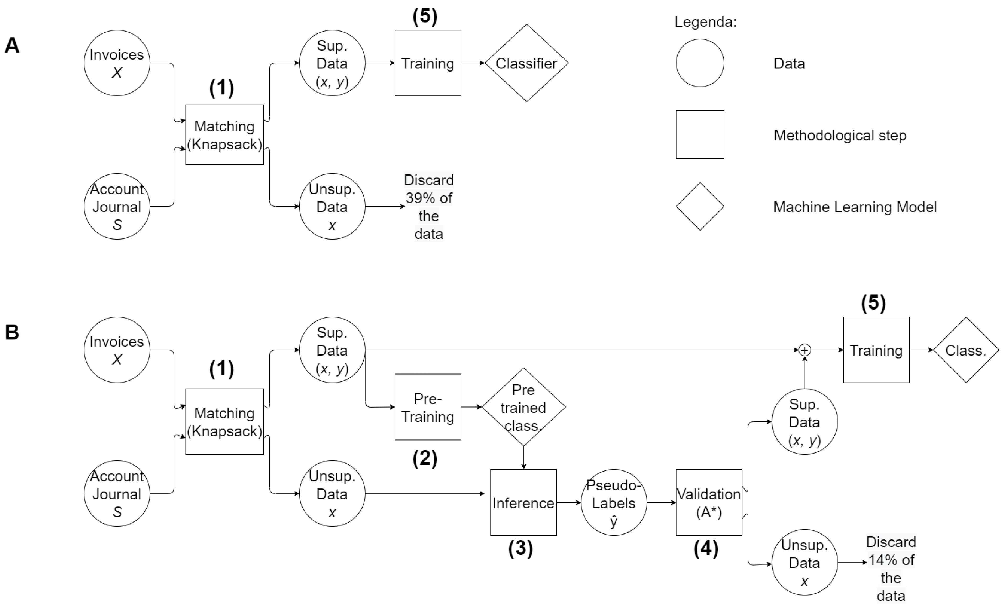
The methodological approach comprises five distinct conceptual steps:
  • Matching—Knapsack Problem: we build the dataset from invoices and journal entries. For every invoice, we set up a combinatorial knapsack problem to assign lines to accounting accounts, resulting in two datasets: a supervised one and an unsupervised one, depending if the knapsack problem is solvable or not.
  • Pre-Training: we train a first version of the Machine Learning classifier on the supervised dataset.
  • Inference: we use the previously trained classifier on the unsupervised dataset to assign a pseudo-label to each line.
  • Pseudo-Labels Validation: we exploit the journal entries to validate the pseudo-labels assigned by the initial classifier. More precisely, the initial classifier prediction is a candidate solution of the knapsack problem at step 1. If the solution solves the knapsack problem we validate the pseudo-labels, otherwise we use a search algorithm to find a valid solution to the knapsack problem.
  • Training: in the final phase, the augmented dataset, now enriched with unsupervised data complemented by pseudo-labels, serves as the foundation for the retraining of the classifier.
Figure 2 highlights how we extended a classical supervised pipeline in solving the invoice labeling problem with our five-steps method.
In this section we will discuss, point by point, the methodology proposed by our work. In fact, we have divided this section into five sub-sections, each of which is dedicated to one of the five methodological steps described by diagram B in the figure above.
Section 4.1 will model the problem of matching documents containing invoices and the account journal as a knapsack problem, highlighting its strengths and weaknesses. Then Section 4.2 will discuss what results can be obtained by training a classification model, which we will refer to as pre-trained, on the data coupled by the knapsack problem. Section 4.3, on the other hand, will introduce the first aspect of strong novelty brought by our work: it will in fact introduce into the pipeline the concept of pseudo-label, that is, the target label inferred by the pre-trained classifier for the unsupervised data. Section 4.4 is the most important in the entire paper because it introduces the A* algorithm as a tool for validating these pseudo-labels. Finally, the methodological discussion is concluded by Section 4.5 which is nothing but a new training on an augmented dataset.

4.1. Matching—Knapsack Problem

The problem of data reconstruction can be addressed exploiting the information about the amounts which are included both in the XML invoices (detailed amounts row by row in column c) and in the accounting journal entry (aggregated amounts in column b). Starting from this point, it is possible to translate the problem at hand into a combinatorial optimization task as the knapsack representation with equality constraints for each invoice [31]. Considering a single invoice X, the combinatorial optimization problem can be formulated as follows:
max j = 1 N k = 1 M z j k s . t . j = 1 N c j z j k = b k , k k = 1 M z j k = 1 , j
where c j is the detailed amount related to the j-th line of the invoice and b k is the aggregated total of the k-th journal entry. The value of the binary variable z j k is 1 if the j-th line of the invoice is associated to the k-th journal entry and in this case we assign to y j the account code of s k . This is the label associated to x j for the following training. Figure 3 shows, with the visual aid of some links representing the associations found as a result of solving the knapsack problem, how to populate the label column.
Considering the rigor of accounting legislation, the knapsack problem can be solved exactly for each invoice, but the difficulty lies in the fact that an invoice often consists of many rows (sometimes even in the hundreds), so the solution matrix Z * of the knapsack problem for the invoice X is to be found in a high-dimensionality space and the resolution is too time-consuming [8].
We will denote by V the set of matched invoices, and by W the set of invoices for which the labels could not be determined, such that V W = U and V W = . A purely supervised approach, in this case, would throw away all unmatched data. Our contribution, on the other hand, lies in being able to also use data from invoices for which the knapsack problem has not been solved, thus using both labelled and unlabelled data for learning in a semi-supervised approach.

4.2. Pre-Training

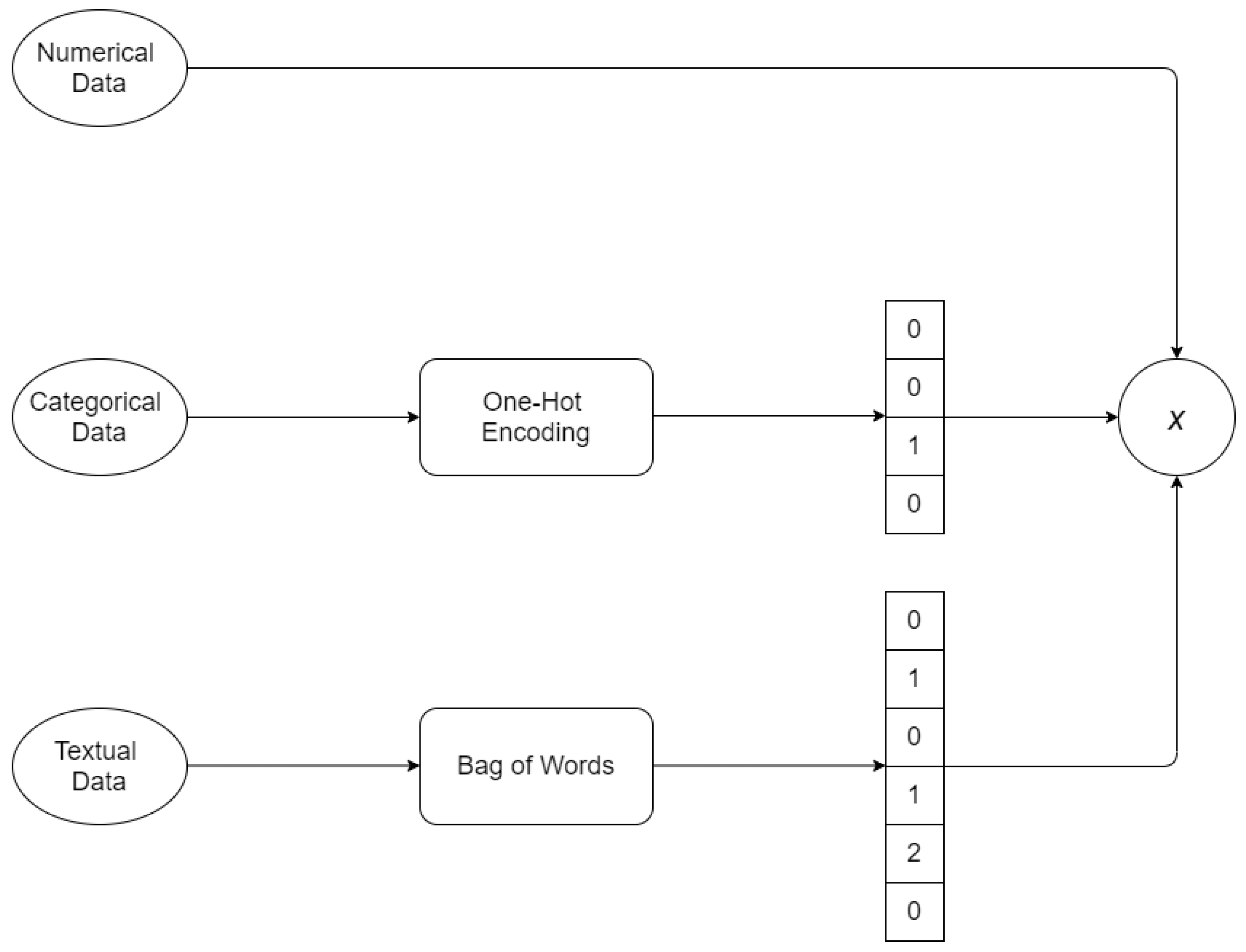
At this stage only rows x j from invoices X in V can be used for learning because they are the only ones for which the label could be determined and so they form pairs ( x j , y j ) : the framework is still fully supervised. After converting all the information in an invoice row into numerical vectors (i.e., for categorical variables the One-Hot Encoding technique was used and for textual information in the description the Bag of Words technique), these pairs were used for training a Machine Learning model. This training allows for the creation of an initial classifier, the accuracy of which will be limited to an extent equal to the number of input-output pairs that we have been able to reconstruct so far.

4.3. Inference

The pre-trained classifier is then used to infer the corresponding account y ^ j to the various rows of invoices in W. The predictions y ^ j are called pseudo-labels and allow for the extension of supervised data collection: this is the essence of semi-supervised learning. However, this positive aspect is countered by the non-absolute reliability of pseudo-labels because of the non perfect accuracy of the pre-trained classifier, which therefore limits the effectiveness of this approach in many areas [32].

4.4. Pseudo-Labels Validation—A*

This section discusses our innovative contribution aimed at eliminating the uncertainty on the pseudo-labels proposed by the pre-trained classifier. This is achieved by bringing our scenario back to the domain of graph search problems.
For each invoice X in W, for which the knapsack problem could not be solved, a vector of pseudo-labels predicted by the pre-trained classifier is now available: y ^ = ( y ^ 1 , . . . , y ^ N ) . To check the accuracy of these, one can group the rows x j according to the associated pseudo-label and calculate the total amount related to an account code, since price c is one of the features for row x j . If these amounts coincide with the aggregated ones (i.e., b) recorded in the accounting journal section S at the respective account code then the pseudo-labels proposed by the pre-trained classifier can be assumed to be correct, otherwise it means that some of them are wrong and must be changed in order not to introduce incorrect data into the dataset. Figure 4 reports, following the same toy example discussed earlier, the two possible aforementioned cases once the pseudo-labels are assigned.
The problem of modifying erroneous pseudo-labels can be traced back to a graph search problem, and thus solved with the A* search algorithm [33]. In order to create this parallelism, certain concepts must be fixed.
  • State Space Definition: the state vector of this problem is y ^ , so the generic node of the graph explored by the search algorithm during its n-th step has a state vector that is denoted by y ^ ( n ) . Each element of this state vector can be assigned to one of the M account codes present in S;
  • Goal Definition: the goal is achieved when the search leads to a node where, by grouping the invoice rows x j according to the pseudo-labels in the state vector y ^ and summing the prices, the same aggregate amounts are found in S, just as in the left-hand panel of Figure 5;
  • Initial State: the search starts from the state vector y ^ ( 1 ) proposed by the pre-trained classifier;
  • Actions: in each state, the range of possible actions is the substitution of one of the pseudo-labels in the state vector with a different account code found in S. Let M be the number of different accounts present in S, then the branching factor for the invoice X, i.e., the number of possible actions in each state, is b f = NM. By way of example only, suppose one of the accounts in S is represented by the code C, then the action modifying the j-th pseudo-label in C will be indicated by C j ;
  • Transition Model: Figure 5 below depicts how the transition from one node to another occurs following the application of an action. The action chosen is the one just presented C j with j = 2 , and therefore changes the second pseudo-label y ^ 2 ( n ) to C, leaving the others unchanged for the ( n + 1 ) -th step;
  • Path Cost: each step on the graph involves the modification of only one element and therefore has a unit cost.
Once the basic concepts are fixed, all that remains is to choose a heuristic to allow the A* algorithm to choose which nodes to explore with priority. The heuristic is a function usually denoted with h that is applied to the state vector of each node and we chose the following rule:
h ( y ^ ) = # e 2 ,
where # e stands for the number of journal entries in S that are not correctly matched by the actual pseudo-labels vector y ^ . This specific heuristic can easily be deduced from a relaxed version of the original problem [34] and is consistent, so the A* algorithm is guaranteed to be optimal in this case [34].
The graph search, which takes up many of the concepts just presented, takes place in a state space of dimension N, in which each variable in the state vector can take on M values. Therefore, the numerosity of the space in which we search for a node that satisfies the goal test is M N : it grows exponentially with the instance of the problem. Given a pre-trained classifier with p accuracy in choosing the pseudo-labels for the initial state y ^ ( 0 ) , we can set:
  • Y B i ( N , p ) stands for the random variable describing the number of rows in X correctly assigned (as a first approximation, we consider the rows x j of the same invoice X to be independent, which allows us to express the sum of Bernoulli variables as a Binomial variable);
  • d stands for the depth of the goal node, i.e., the distance in steps between the initial node and the goal node along the optimal path;
it holds that
E [ d ] = N E [ Y ] = ( 1 p ) N
because each step on the graph fixes an incorrect pseudo-label.
Depending on the value of d and the numerosity of the search space the time required for A* to reach a goal node is different. A maximum threshold waiting time must be established, and given an invoice X, if A* converges before the threshold time, the pseudo-labels are validated and become actual labels. Suppose, for example, we reach the goal for invoice X after n * steps, then certified labels can be entrusted to the invoice rows by using as target variables the last explored vector of pseudo-labels, i.e., imposing y = y ^ ( n * ) .

4.5. Training

At the end of running A* to validate the pseudo-labels for each invoice in W, new supervised data are obtained to add to those already collected and new training can be done on a larger dataset. The result of this is a classifier with greater ability to generalize to unseen data.
Instead, in the cases of invoices for which the pseudo-labels proposed by the pre-trained classifier were excessively low quality and thus the search algorithm took too long to converge the corresponding rows are discarded from the dataset, but still this waste is significantly smaller than in the baseline framework.

5. Experiments

5.1. Data Pre-Processing

Data pre-processing covers both the invoices in V and those in W because, as we said, the unsupervised data do not get thrown away. First of all, for each row x j in X only the information with predictive power on the target variable had to be selected, in what is called the feature selection phase. Then, of course, much of this information has to undergo some reworking steps in order to be used as features in a machine learning algorithm. Three types of data can be identified:
  • Numerical data: are used as they are (e.g., total price, tax rate);
  • Categorical data: are converted into a numerical vector thanks to a One-Hot Encoding procedure [35] (e.g., code of the business partner, method of payment);
  • Textual data: are transformed into a numeric vector thanks to the Bag of Words approach [36] (e.g., description of the invoice row, which contains very important information for deducing the nature of the product or service exchanged).
The result of this step is a purely numerical vector (as observed in Figure 6), and thus comprehensible to an artificial intelligence algorithm.

5.2. Pipeline Application

The previously described methodological pipeline was applied to our real case, giving the following results.
  • Matching—Knapsack Problem: for many invoices the knapsack problem described in Equation (1) is not solvable. To be precise the input-output relationship was reconstructed without any ambiguity only for 61% of the invoice rows available in the raw dataset giving pairs ( x j , y j ) , thus the discard rate is 39%;
  • Pre-Training: The multi-class classification problem that the model must learn to solve is the association of an account code y j with the vector x j . Since a large amount of data was not available, Deep Learning models, which require a lot of data to learn [37], were excluded. Several of the best models available in the literature and in the Python Scikitlearn library for multi-class classification were tried out: Support Vector Machine (SVM) [38], Naïve Bayes [39], Decision Tree [40], Random Forest [41] and AdaBoost [42]. The performances of these models were assessed by means of a 10-fold cross-validation and, of all, the models based on an ensemble of trees proved to be the best for this task. In fact, already in this initial training on a limited supervised dataset they achieved an accuracy of 91%. The quantitative results recorded during the experiments will be discussed in more detail in the next section, also with the support of tables and images;
  • Inference: the pre-trained classifier was then used to infer the pseudo-label for the lines of the invoices in W;
  • Pseudo-Labels Validation—A*: thanks to the high accuracy of the pre-trained classifier, most of the pseudo-labels were correct. As a consequence, referring to Equation (3), the search has to be done on a shallow tree and A* converged in most of the cases (out of 1156 unlabeled data, 747 got a label thanks to this procedure).
However, the reader may be interested to understand why in some cases the search algorithm does not converge. Excluding the trivial case where there are errors in the entries of amounts c or b, non-convergence can also occur when the search takes too long.
A practical example we have encountered is the following.
One of the invoices in our dataset D has N = 34 rows and the corresponding journal entry has M = 4 accounts. This means that the space in which the search for the correct labels takes place is immense: it has 4 34 nodes to explore.
Now, even if the pre-trained classifier has good accuracy and correctly estimates the accounting account for most of the 34 rows, there is still a computationally expensive exploration to be done. For example, if the classifier makes 4 errors, the goal node is 4 steps away (i.e., 4 pseudo-labels have to be modified) but in such a large space even a 4-step exploration is unfeasible. In fact, each of the swaps may involve changing one of the 34 pseudo-labels by assigning it 4 different accounts; this means that at each step 34 × 4 = 136 (branching factor) new nodes may be explored.
The following Figure 7 is only intended to visually show the exponential nature of the growth in the number of nodes explored during the search. It is a very simplified case with N = 2 and M = 3 (the 3 possible accounts are only A, B and C) but nevertheless shows the complexity of the problem (Obviously some nodes are repeated and A* explores the graph using intelligent heuristics in order to favour promising paths, so not all nodes shown in the figure would be tested. We repeat that the figure is purely illustrative to give the reader an idea of how the search space expands, especially in scenarios with large N and M values).
Lines belonging to invoices for which even A* cannot solve the matching problem are 14% and cannot be used in this automatic system. The only scenario in which information could be extracted from them would involve processing them manually under the supervision of an accountant to match them to the correct account before entering them into dataset D, but this is extremely time consuming.
5.
Training: the same model was trained and evaluated for the second time and improved the accuracy between 1% and 4%, depending on its data efficiency.

5.3. Quantitative Results

Table 2 is intended to show the improvement in accuracy (we chose this metric as a reference for its ease of interpretation) with the proposed methodology by means of an ablation test.
We report the performance of the five tested classifiers in three frameworks:
  • Supervised Framework: only data for which the knapsack problem has reconstructed the input-ouptut relation are used. This is the baseline method with which this problem has been approached so far in the literature [8]. It basically consists in applying only steps 1 and 5 of the entire pipeline: refer to diagram A in Figure 2.
  • Standard Semi-Supervised Framework: in a classic semi-supervised approach, pseudo-labels are inferred by the pre-trained classifier and may not be correct, introducing noise into the dataset D. This method corresponds to steps 1, 2, 3 and 5.
  • Semi-Supervised Framework + A*: this is the innovative framework we propose in which only data with certified labels are used, visually described by diagram B in Figure 2.
This triple test highlights the importance of introducing the pseudo-label validation step with A*. In fact, note that, without A*, accuracy remains unchanged for tree-based models while it even worsens for SVM and Naïve Bayes as the positive effect of increasing the dataset is offset by the introduction of erroneous labels.
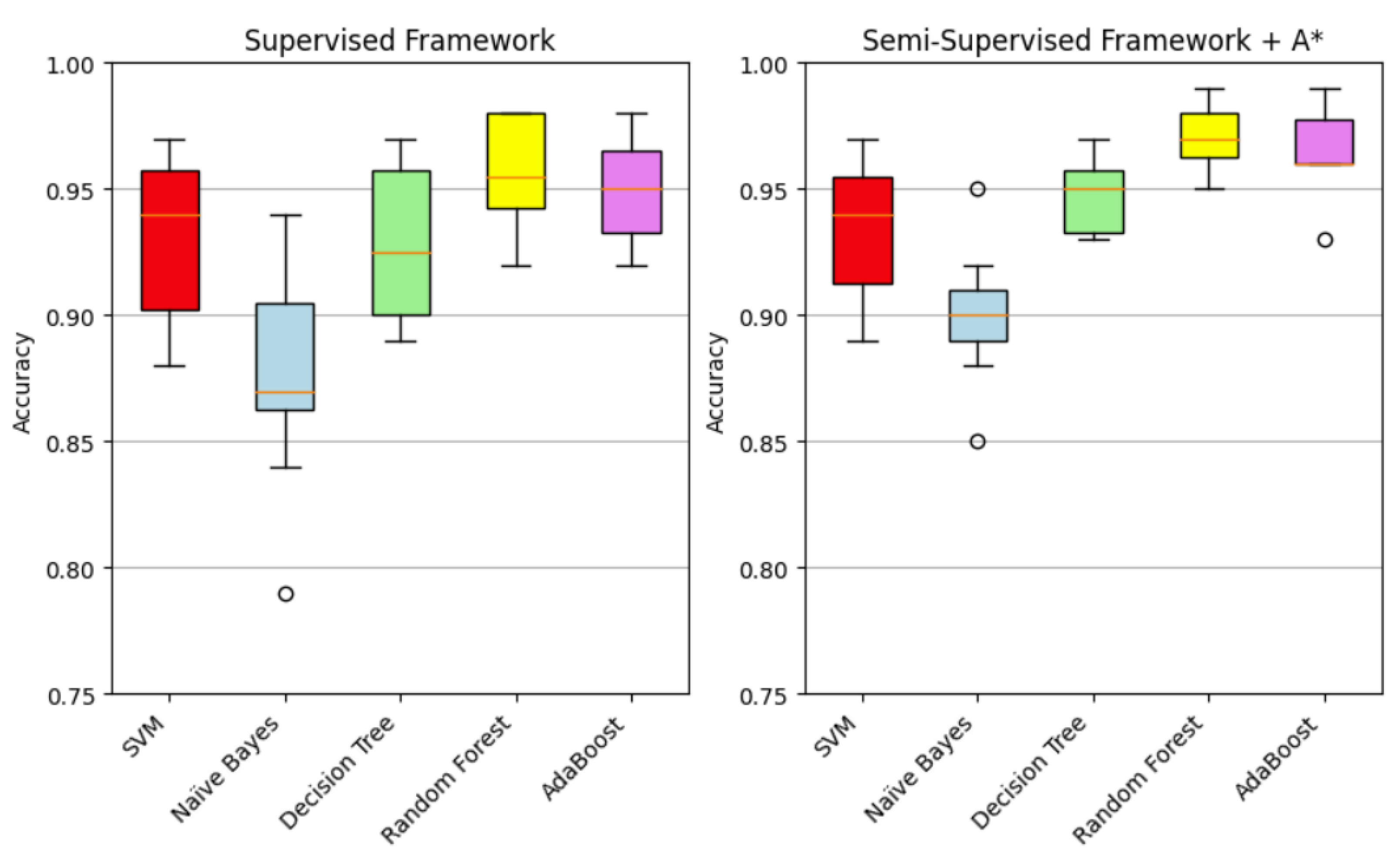
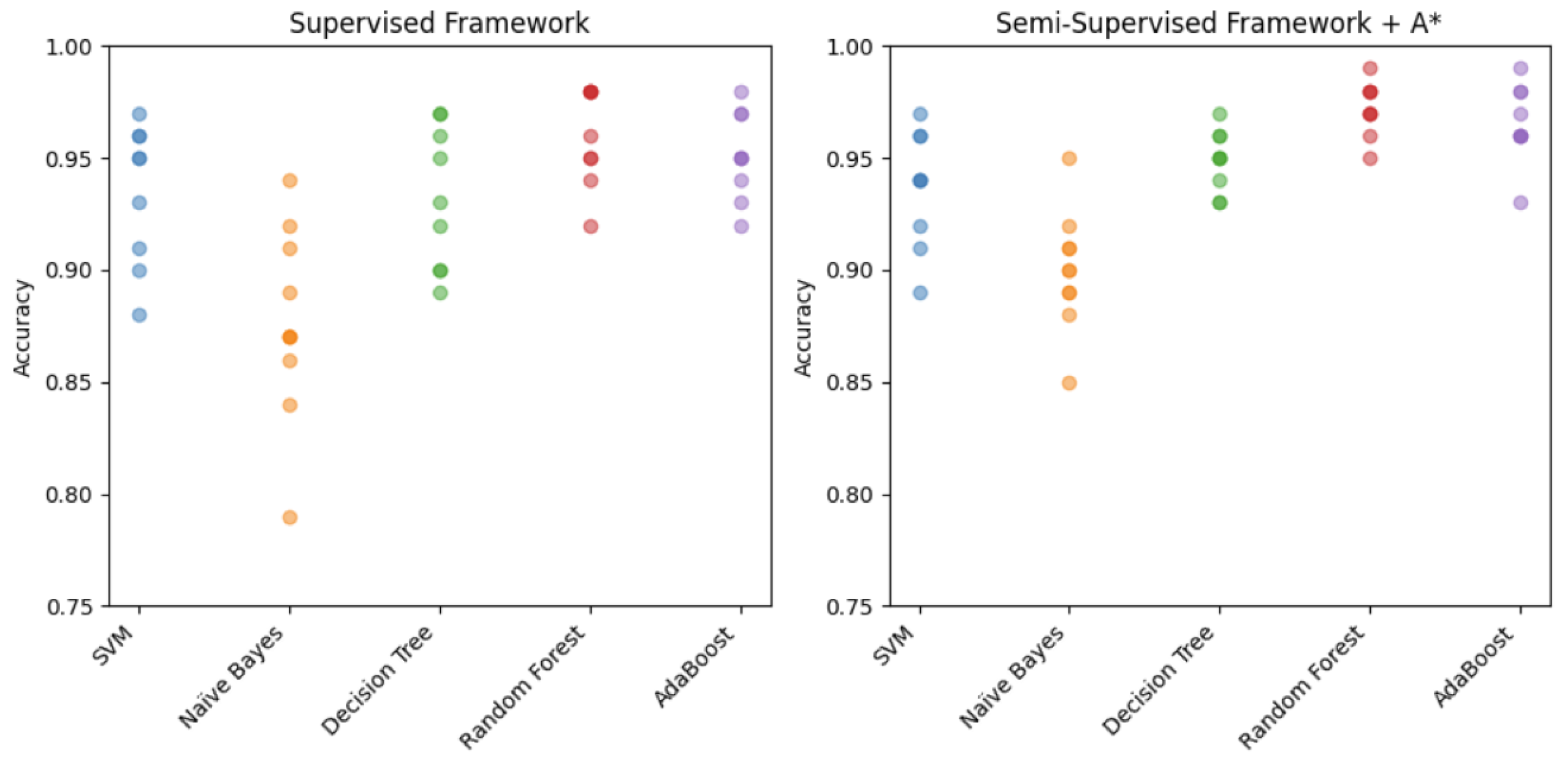
Figure 8 and Figure 9 refer to the first and third frameworks presented. By means of boxplots and scatter plots respectively, these two figures show the increase in accuracy recorded for each of the models tested with a 10-folds cross-validation.
It quickly becomes apparent that all models perform better in the semi-supervised framework we introduced in this work, which is not surprising since it allows training on a larger reliable dataset. Some models benefit more from the enlargement of the supervised dataset and others less, with an increase in accuracy between 1% (SVM) and 4% (Decision Tree). As anticipated, the models that prove to be best suited for this problem are Random Forest and AdaBoost, both of them based on an ensemble of trees.
Focusing on one of these, Table 3 is dedicated to provide broader information on the performance of Random Forest, not only under the accuracy point of view, in the proposed semi-supervised framework (What immediately jumps out at you is how the metrics are drastically lower when the test is done on Fold 1 (and the same thing happens with the other classifiers too but for visual reasons in Figure 8 and Figure 9 we have focused only on the range where most of the measurements fall). This can be explained by remembering how GroupKFold function from scikitlearn works: lines of the same invoice are not allowed to be in different folds, to avoid training and validation on entries of the same invoice. In Fold 1 there are all 125 rows of the largest invoices. These all have the same label and are the only ones with that label in the whole dataset, so the model is trained on the other nine folds and does not learn to recognise this specific label, committing many errors when validated on Fold 1. Ignoring this particular fold, the Random Forest’s accuracy would even rise to 97% on average).
Furthermore, in the key performance table of our study, denoted as Table 4, we show from a quantitative point of view the improvements achieved by the semi-supervised approach coupled with A*. On the one hand, we have an improvement in the accuracy of the classifiers, which, however, cannot be of great magnitude since the pre-trained classifiers already provided very good performance; on the other hand, we have what we think is the most important result, which is the recovery of a lot of data that could not be used without our pipeline: something that would be valuable in any machine learning problem.

6. Conclusions and Discussion

6.1. Result Discussion

The effectiveness of the presented method lies in the comparison of the purely supervised framework and the semi-supervised framework with A*. As far as we know, the best performance on a similar task are form the work of Bardelli et al. [8], which operates in the Italian accounting context just like we do, and adopts a fully supervised framework. In their work, the data discard rate is 39% and the performance on received invoice line classification is 89.8 % f1-score. In our experiment, first we replicated the same pipeline achieving a similar discard rate and f1-score. However, with our proposed method, we were able to substantially reduce the discard rate to 14%, consequently achieving a f1-score of 92 % . Additionally, our performance is quite competitive, nearing the level achieved by Ref. [22] at 95.5 % . However, direct performance comparison is challenging as we did not have access to the additional features from bank accounts that were available to them.
Then, we conducted a deeper investigation into the impact of the A* search algorithm with an ablation experiment. In this experiment, we trained all the classifiers with a standard semi-supervised procedure, excluding the A* component. Interestingly, the performance of the classifiers remains unchanged or exhibited slight deterioration compared to the performance of the supervised framework. This is a well know drawback of semi-supervised learning and it has been identified in the literature [9]. The introduction of unverified unlabeled can inadvertently introduce noise, contributing to performance degradation. The impact of the noise is different on each of the classifiers, having a larger degradation on more sensitive algorithm such the SVM [43].
Finally, it is worth noting how the quality and quantity of the dataset may impact on the performance. As far as accuracy is concerned, we achieved comparable performance while working with a dataset that has a quantity of samples in the order of thousands, compared to [8] that has in the order of hundreds of thousands. However, the experiments proved the size of the dataset is sufficiently large to represent the distribution of the data and correctly train the classifiers. On the other hand, the quality of the data is a pivotal tole to the successful application of machine learning, as underscored by our proposed ablation experiment.
Unfortunately, due to the sensitive nature of the data, there is no benchmark dataset in this area on which to compare methods. The fact that we only had access to a small amount of data is what motivated us from the start to make the best use of it, trying to label the largest fraction of it and thus be able to train an effective model.

6.2. Work Summary

Machine learning has emerged as a valuable tool for enhancing business operations, and in this article, we delved into its potential to assist in the execution of typical tasks handled by accountants. Our exploration aimed to showcase how this technology could simplify and complement the work of human operators in the field.
We started from a real-world problem: the classification of electronic invoice entries. We developed and trained a classifier to tackle this challenge. However, recognizing the potential of the vast volume of unsupervised data available, we embarked on a mission to take advantage of this resource more effectively. This led us to experiment a semi-supervised learning framework, a powerful approach that extends beyond the limitations of traditional supervised methods.
Yet, this transition came with its own set of challenges, primarily centered around the introduction of uncertainly labeled data into our dataset. To address these complexities, we designed a methodological framework that revolves around the principles of semi-supervised learning and utilizes a graph search algorithm, A*. This framework overcomes the pseudo-label generation challenges by leveraging the group-instance structure of the data, consequently impacting the accuracy of the classifiers. In fact, as we enriched our training set with new, unambiguously reconstructed input-output pairs, we witnessed significant improvements in the performance of the classifiers. This transformation allowed our model to improve SOTA accuracy in assigning account codes to the transactions encapsulated within the XML invoice rows.
In essence, our exploration showcased the potential of machine learning as a powerful ally in streamlining complex accounting tasks. It exemplified how a combination of innovative techniques, including semi-supervised learning and data refinement, can lead to substantial enhancements in classification accuracy and, ultimately, operational efficiency.

6.3. Future Works

Nonetheless, despite the promising results achieved by our work, there is a large margin for improvement regarding the application of machine learning in corporate accounting. First, in our work, we applied shallow learning techniques and feature engineering because of the size of the data available for the study. It would be interesting to evaluate deep learning algorithms and text embeddings, such as Word2Vec or LLM; these paradigms would benefit from larger datasets and lead to sensibly improving performance. Second, we should look for integrating other sources of information into the dataset, e.g., financial transaction, corporate descriptions, market data, law descriptions, and so on, because a lot of important features for the task depend on the context and are not usually available. Finally, in this study we proposed a single iteration of the algorithm, however it is possible to further refine the pseudo-labels by repeating the steps 2, 3, 4, before the final training at step 5. Moreover, it could be extremely useful to develop an active learning system that query the human expert accountant about “difficult” invoice to improve the quality of the dataset.
On the other hand, the proposed approach arose from a problem related to the accounting world but can be repurposed in a multitude of contexts. In general, the methodology illustrated brings benefits where there is unsupervised data and one wants to certify the validity of the labels proposed by a classifier. These labels to be certified can be either pseudo-labels in a semi-supervised framework, as presented in this article, or predictions on test data, as long as one can define a goal condition with which to stop the search on the state vector graph being certain that the actual labels are correct.
In this regard, an interesting future research direction would be to identify other practical problems with this structure and, after modeling them, apply the same pipeline described in the article, observing the increase in accuracy as introducing new data. A macro-category of problems in which we can find a similar structure is where the samples are grouped into groups, on which an aggregate condition can be placed (just like the amounts recorded in each account in the invoice problem described above). For example, this can be done with temporal data grouped weekly, monthly, or annually, or with spatial data grouped geographically. Another more interesting and appropriate case in which much research has been done [44] is the link prediction problems on graphs.
Concerning the latter, the aim is to use machine learning techniques to predict the existence of certain links in the graph: it is therefore a binary 0 / 1 classification problem [45]. The links can be naturally grouped according to the nodes they touch and, in cases where the number of links touching a certain node is known as the aggregate condition on the group, it is possible to swap the labels initially predicted by the classifier model by starting a search with A* until the aggregate condition is matched. Purely as an inspiration for further research in this direction, we point out concrete cases of link prediction on social networks (each node represents a person) where this condition can realistically be encountered: co-authorship in scientific publications [46], collaboration on a project within a large company, membership of a common board of directors. In all these cases, it is likely to know the number of links relative to each node in the network, but one may be wondering which of the total possible links exist.

Author Contributions

Conceptualization, A.L. and B.P.; methodology, A.L and B.P.; software, A.L. and B.P.; validation, B.P.; formal analysis, B.P.; investigation, A.L. and B.P.; resources, A.L. and B.P.; data curation, A.L. and B.P.; writing—original draft preparation, B.P.; writing—review and editing, A.L. and B.P.; visualization, B.P.; supervision, A.L; project administration, A.L.; funding acquisition, A.L. All authors have read and agreed to the published version of the manuscript.

Funding

We gratefully acknowledge the support and funding provided by Polaris Engineering Spa and Prime Office Srl for this research. Polaris Engineering Spa generously funded the research project, including the publication fees (APC—Article Processing Charges). Additionally, we would like to express our gratitude to Prime Office for providing the dataset used in this study. Their contribution was instrumental in enabling the empirical analysis and findings presented in this paper. We are grateful for their collaboration and assistance throughout the research process.

Data Availability Statement

Restrictions apply to the availability of these data. Data was obtained from Prime Office S.r.l. and are available from Polaris Engineering S.p.a. with the permission of Prime Office.

Acknowledgments

We would like to extend our sincere appreciation to Giulia and Francesca from the administration division of Polaris Engineering Spa for their invaluable support and suggestions throughout the course of this research. Their expertise and guidance played a crucial role in navigating the administrative aspects of the project and ensuring its successful execution. We are truly grateful for their dedication and assistance, which significantly contributed to the completion of this study.

Conflicts of Interest

The authors declare no conflict of interest.

Appendix A. Glossary

In this appendix, we present a comprehensive table (Table A1) that enumerates the various variables employed in our study, accompanied by detailed descriptions elucidating their roles and significance.
Table A1. Variables overview.
Variable NameVariable Description
DDataset
XInvoices
SAccount journal dedicated to invoices registration
xInvoice line
sJournal line that represents the registration in a specific account
iIndex to identify a specific invoice and the corresponding journal section
jRow index inside an invoice
kRow index inside a journal section
NNumber of lines in an invoice
MNumber of lines in a journal section
yTrue target label for an invoice line
y ^ Target label inferred by the classifier for a single invoice line
y ^ Vector with all the target labels inferred for an invoice
cNumerical value associated to an invoice line (i.e., price)
bNumerical value associated to a journal line
zBinary variable of the knapsack problem
ZMatrix collecting all the binary variables for an invoice X
USet of all the invoice indexes
VSubset of all the invoice indexes for which the knapsack problem has been
solved
WSubset of all the invoice indexes for which the knapsack problem has not
been solved
nStep of the searching algorithm
hHeuristic function
dDistance of the solution node on the graph from the initial state
# e Number of wrong predictions in y ^
n * Number of steps required to conclude the search

Appendix B. Data Description

In this appendix, we provide a quick exposition on the real data used throughout our research. These data sources form the bedrock of our analysis, and thus, understanding their structure can help for a deep understanding of the methodologies and findings presented in the main body of this work. By offering a closer look at the raw data, we hope to provide the reader with an enhanced perspective on the real-world challenges encountered and the preprocessing steps necessitated before embarking on the core analysis.
The raw data we worked with are:
Both data sources were pre-processed in order to bring them into a tabular format for later analysis. Below, in Table A2 and Table A3, is an example of an invoice and the corresponding journal entry in tabular form. Note that, for simplicity’s sake, we only show the text description and price of each line of the invoice, whereas the original document would have hundreds of fields. Furthermore, some words in the description have been darkened with asterisks because they are data of a sensitive nature. For this same reason, we cannot provide access to the entire dataset D we have used.
We have chosen as an example an invoice with 27 lines relating to 27 products sold, whose corresponding entry in the journal involves 5 accounts. Therefore, referring to the article notation, in this case N = 27 and M = 5.
Table A2. Simplified example of an invoice in tabular format.
No.DescriptionPrice
0**** LIEVITO FRESCO PAKMAYA PZ 500 GR19.80
1**** CODA ARAGOSTA–MICRO CT 7 KG COD.AK...40.13
2PAC GEL SFOGLIATA RICCIA MIGNON GR 30 CT 5 KG24.47
3PAC GEL SFOGLIATA SEMIDOLCE RUSTICA CT 4 KG17.96
4RISPO RUSTICI MIGNON CF 2.5 KG25.00
5**** TAPPI GRANDI CT 150 PZ19.61
6***** FARINA–TIPO AMERICANA CARTA CF 25 KG36.40
7****** FARINA–TIPO 00 EXTRA CF 25 KG25.95
8VANDEMOORTELE MIX GOLD CUP CROISSANT CF …61.91
9CELLOPHANE & PAPER CARTA DA FORNO 40 × 60 CF 500PZ17.84
10GOURMET LINE MIX CREAM AMIDO CF 10 KG28.48
11**** NOCCIOLATA ***** CF 13 KG COD. 101015148.35
12TORRENTE ****** CT 3X4.1 KG11.04
13******* CIGARETTES SURPRISE CT 1,5 KG21.24
14******* CANNOLI CIOCCOLATO MIGNON CT 3.5 KG31.23
15****** ANANAS MIGNON 33 FETTE CF 850 GR9.55
16IRCA **** NEUTRO CF 1KG COD.705085.85
17****** PIROTTINI TONDI COLORATI MIS. 3 H 18.5...7.10
18IRCA CHOCOCREAM ***** PISTACCHIO ***** CF KG 5...44.36
19SALVI PIATTI ALA ORO CM 26 CF 10 KG15.40
20PININ PERO ZUCCHERO VELO CF 5 KG4.79
21IRCA SCAGLIETTA ***** PURO FONDENTE ***** CF 1...5.12
22***** SEMOLA DI GRANO DURO **RIPIENO SFOGLIA...4.34
23******* PREP. VEG. HOPLA’ EASY TOP 1LT61.94
24SWEET D.e D. ZUCCHERO CF 25 KG15.41
25REVIVA PIROTTINI OVALI COLORATI MIS 3 CF 1000 PZ5.52
26Spese Varie0.30
Table A3. Example of journal registration.
CodeAccount NameAmount
66/05/006MATERIE PRIME C/ACQ. P/PROD.SERV.445.4
66/20/005MATERIE DI CONSUMO C/ACQUISTI65.47
66/25/509FARINA66.69
66/25/006MERCI C/ACQUISTI P/PROD.SERV.31.23
66/30/055SPESE ACCESSORIE SU ACQUISTI0.3
As can be seen from this example, the invoice lines are aggregated into accounts. For this reason, labels are only available at group level.

References

  1. Frey, C.B.; Osborne, M.A. The future of employment: How susceptible are jobs to computerisation? Technol. Forecast. Soc. Chang. 2017, 114, 254–280. [Google Scholar] [CrossRef]
  2. Tater, T.; Gantayat, N.; Dechu, S.; Jagirdar, H.; Rawat, H.; Guptha, M.; Gupta, S.; Strak, L.; Kiran, S.; Narayanan, S. AI Driven Accounts Payable Transformation. Proc. AAAI Conf. Artif. Intell. 2022, 36, 12405–12413. [Google Scholar] [CrossRef]
  3. Koch, B. E-Invoicing/E-Billing. Significant Market Transition Lies Ahead. Billentis. 2017. Available online: https://www.billentis.com/einvoicing_ebilling_market_report_2017.pdf (accessed on 14 September 2023).
  4. Cedillo, P.; García, A.; Cárdenas, J.D.; Bermeo, A. A Systematic Literature Review of Electronic Invoicing, Platforms and Notification Systems. In Proceedings of the 2018 International Conference on eDemocracy & eGovernment (ICEDEG), Ambato, Ecuador, 4–6 April 2018; pp. 150–157, ISSN: 2573-1998. [Google Scholar] [CrossRef]
  5. Poel, K.; Marneffe, W.; Vanlaer, W. Assessing the electronic invoicing potential for private sector firms in Belgium. Int. J. Digit. Account. Res. 2016, 16, 8517. [Google Scholar] [CrossRef] [PubMed]
  6. Bergdorf, J. Machine Learning and Rule Induction in Invoice Processing: Comparing Machine Learning Methods in Their Ability to Assign Account Codes in the Bookkeeping Process. Available online: http://urn.kb.se/resolve?urn=urn:nbn:se:kth:diva-235931 (accessed on 14 September 2023).
  7. Azman, N.A.; Mohamed, A.; Jamil, A.M. Artificial Intelligence in Automated Bookkeeping: A Value-added Function for Small and Medium Enterprises. JOIV Int. J. Inform. Vis. 2021, 5, 224–230. [Google Scholar] [CrossRef]
  8. Bardelli, C.; Rondinelli, A.; Vecchio, R.; Figini, S. Automatic Electronic Invoice Classification Using Machine Learning Models. Mach. Learn. Knowl. Extr. 2020, 2, 617–629. [Google Scholar] [CrossRef]
  9. van Engelen, J.E.; Hoos, H.H. A survey on semi-supervised learning. Mach. Learn. 2020, 109, 373–440. [Google Scholar] [CrossRef]
  10. Cho, S.; Vasarhelyi, M.A.; Sun, T.S.; Zhang, C.A. Learning from Machine Learning in Accounting and Assurance. J. Emerg. Technol. Account. 2020, 17, 10718. [Google Scholar] [CrossRef]
  11. Bertomeu, J. Machine learning improves accounting: Discussion, implementation and research opportunities. Rev. Account. Stud. 2020, 25, 1135–1155. [Google Scholar] [CrossRef]
  12. Tarawneh, A.S.; Hassanat, A.B.; Chetverikov, D.; Lendak, I.; Verma, C. Invoice Classification Using Deep Features and Machine Learning Techniques. In Proceedings of the 2019 IEEE Jordan International Joint Conference on Electrical Engineering and Information Technology (JEEIT), Amman, Jordan, 9–11 April 2019; pp. 855–859. [Google Scholar] [CrossRef]
  13. Ha, H.; Horák, A. Information extraction from scanned invoice images using text analysis and layout features. Signal Process. Image Commun. 2021, 102, 116601. [Google Scholar] [CrossRef]
  14. Li, M. Smart Accounting Platform Based on Visual Invoice Recognition Algorithm. In Proceedings of the 2022 6th International Conference on Computing Methodologies and Communication (ICCMC), Erode, India, 29–31 March 2022; pp. 1436–1439. [Google Scholar] [CrossRef]
  15. Subramani, N.; Matton, A.; Greaves, M.; Lam, A. A Survey of Deep Learning Approaches for OCR and Document Understanding. arXiv 2021, arXiv:2011.13534. [Google Scholar]
  16. Thorat, C.; Bhat, A.; Sawant, P.; Bartakke, I.; Shirsath, S. A Detailed Review on Text Extraction Using Optical Character Recognition. In Proceedings of the ICT Analysis and Applications; Lecture Notes in Networks and Systems. Fong, S., Dey, N., Joshi, A., Eds.; Springer: Singapore, 2022; pp. 719–728. [Google Scholar] [CrossRef]
  17. Ding, K.; Lev, B.; Peng, X.; Sun, T.; Vasarhelyi, M.A. Machine learning improves accounting estimates: Evidence from insurance payments. Rev. Account. Stud. 2020, 25, 1098–1134. [Google Scholar] [CrossRef]
  18. Li, Z.; Zheng, L. The Impact of Artificial Intelligence on Accounting; Atlantis Press: Sanya, China, 2018; ISSN 2352-5398. [Google Scholar] [CrossRef]
  19. Johansson, S. Classification of Purchase Invoices to Analytic Accounts with Machine Learning. Master Thesis, Aalto University, Espoo, Finland, 2022. Available online: https://aaltodoc.aalto.fi/bitstream/handle/123456789/119486/master_Johansson_Samuel_2023.pdf?sequence=1&isAllowed=y (accessed on 14 September 2023).
  20. Bengtsson, H.; Jansson, J. Using Classification Algorithms for Smart Suggestions in Accounting Systems. Available online: https://hdl.handle.net/20.500.12380/219162 (accessed on 14 September 2023).
  21. Kieckbusch, D.S.; Filho, G.P.R.; Di Oliveira, V.; Weigang, L. Towards Intelligent Processing of Electronic Invoices: The General Framework and Case Study of Short Text Deep Learning in Brazil. In Proceedings of the Web Information Systems and Technologies, Porto, Portugal, 25–27 April 2023; Lecture Notes in Business Information Processing. Marchiori, M., Domínguez Mayo, F.J., Filipe, J., Eds.; Springer: Cham, Switzerland, 2023; pp. 74–92. [Google Scholar] [CrossRef]
  22. Munoz, J.; Jalili, M.; Tafakori, L. Hierarchical classification for account code suggestion. Knowl.-Based Syst. 2022, 251, 109302. [Google Scholar] [CrossRef]
  23. Severin, K.; Gokhale, S.; Dagnino, A. Keyword-Based Semi-Supervised Text Classification. In Proceedings of the 2019 IEEE 43rd Annual Computer Software and Applications Conference (COMPSAC), Milwaukee, WI, USA, 4–8 June 2019; pp. 417–422. [Google Scholar] [CrossRef]
  24. Gururangan, S.; Dang, T.; Card, D.; Smith, N.A. Variational Pretraining for Semi-supervised Text Classification. arXiv 2019, arXiv:1906.02242. [Google Scholar]
  25. Johnson, R.; Zhang, T. Supervised and Semi-Supervised Text Categorization using LSTM for Region Embeddings. In Proceedings of the 33rd International Conference on Machine Learning, PMLR, New York, NY, USA, 19–24 June 2016; pp. 526–534, ISSN: 1938-7228. [Google Scholar]
  26. Miyato, T.; Dai, A.M.; Goodfellow, I. Adversarial Training Methods for Semi-Supervised Text Classification. arXiv 2021, arXiv:1605.07725. [Google Scholar]
  27. Berthelot, D.; Carlini, N.; Goodfellow, I.; Papernot, N.; Oliver, A.; Raffel, C.A. MixMatch: A Holistic Approach to Semi-Supervised Learning. In Proceedings of the Advances in Neural Information Processing Systems, Long Beach, CA, USA, 4–9 December 2019; Curran Associates, Inc.: Long Beach, CA, USA, 2019; Volume 32. [Google Scholar]
  28. Ouali, Y.; Hudelot, C.; Tami, M. An Overview of Deep Semi-Supervised Learning. arXiv 2020, arXiv:2006.05278. [Google Scholar]
  29. Gong, C.; Tao, D.; Liu, W.; Liu, L.; Yang, J. Label Propagation via Teaching-to-Learn and Learning-to-Teach. IEEE Trans. Neural Netw. Learn. Syst. 2017, 28, 1452–1465. [Google Scholar] [CrossRef]
  30. Iscen, A.; Tolias, G.; Avrithis, Y.; Chum, O. Label Propagation for Deep Semi-supervised Learning. arXiv 2019, arXiv:1904.04717. [Google Scholar] [CrossRef]
  31. Assi, M.; Haraty, R. A Survey of the Knapsack Problem. 2018. Available online: https://ieeexplore.ieee.org/document/8672677 (accessed on 14 September 2023).
  32. Rizve, M.N.; Duarte, K.; Rawat, Y.S.; Shah, M. In Defense of Pseudo-Labeling: An Uncertainty-Aware Pseudo-label Selection Framework for Semi-Supervised Learning. arXiv 2021, arXiv:2101.06329. [Google Scholar]
  33. Candra, A.; Budiman, M.A.; Hartanto, K. Dijkstra’s and A-Star in Finding the Shortest Path: A Tutorial. In Proceedings of the 2020 International Conference on Data Science, Artificial Intelligence, and Business Analytics (DATABIA), Medan, Indonesia, 16–17 July 2020; pp. 28–32. [Google Scholar] [CrossRef]
  34. Russell, S.J.; Norvig, P. Artificial Intelligence: A Modern Approach, 4th ed.; Pearson Series in Artificial Intelligence; Pearson: Hoboken, NJ, USA, 2021. [Google Scholar]
  35. Seger, C. An Investigation of Categorical Variable Encoding Techniques in Machine Learning: Binary versus One-Hot and Feature Hashing. Available online: https://urn.kb.se/resolve?urn=urn:nbn:se:kth:diva-237426 (accessed on 14 September 2023).
  36. Zhang, Y.; Jin, R.; Zhou, Z.H. Understanding bag-of-words model: A statistical framework. Int. J. Mach. Learn. Cybern. 2010, 1, 43–52. [Google Scholar] [CrossRef]
  37. Pasupa, K.; Sunhem, W. A comparison between shallow and deep architecture classifiers on small dataset. In Proceedings of the 2016 8th International Conference on Information Technology and Electrical Engineering (ICITEE), Yogyakarta, Indonesia, 5–6 October 2016; pp. 1–6. [Google Scholar] [CrossRef]
  38. Suthaharan, S. Support Vector Machine. In Machine Learning Models and Algorithms for Big Data Classification: Thinking with Examples for Effective Learning; Suthaharan, S., Ed.; Integrated Series in Information Systems; Springer: Boston, MA, USA, 2016; pp. 207–235. [Google Scholar] [CrossRef]
  39. Yang, F.J. An Implementation of Naive Bayes Classifier. In Proceedings of the 2018 International Conference on Computational Science and Computational Intelligence (CSCI), Las Vegas, NV, USA, 12–14 December 2018; pp. 301–306. [Google Scholar] [CrossRef]
  40. Priyanka; Kumar, D. Decision tree classifier: A detailed survey. Int. J. Inf. Decis. Sci. 2020, 12, 246–269. [Google Scholar] [CrossRef]
  41. Rigatti, S.J. Random Forest. J. Insur. Med. 2017, 47, 31–39. [Google Scholar] [CrossRef] [PubMed]
  42. Schapire, R.E. Explaining AdaBoost. In Empirical Inference: Festschrift in Honor of Vladimir N. Vapnik; Schölkopf, B., Luo, Z., Vovk, V., Eds.; Springer: Berlin/Heidelberg, Germany, 2013; pp. 37–52. [Google Scholar] [CrossRef]
  43. Schooltink, W.T. Testing the Sensitivity of Machine Learning Classifiers to Attribute Noise in Training Data; University of Twente: Twente, The Netherlands, 2020. [Google Scholar]
  44. Hasan, M.A.; Zaki, M.J. A Survey of Link Prediction in Social Networks. In Social Network Data Analytics; Aggarwal, C.C., Ed.; Springer: Boston, MA, USA, 2011; pp. 243–275. [Google Scholar] [CrossRef]
  45. Lü, L.; Zhou, T. Link prediction in complex networks: A survey. Phys. A Stat. Mech. Its Appl. 2011, 390, 1150–1170. [Google Scholar] [CrossRef]
  46. Chuan, P.M.; Son, L.H.; Ali, M.; Khang, T.D.; Huong, L.T.; Dey, N. Link prediction in co-authorship networks based on hybrid content similarity metric. Appl. Intell. 2018, 48, 2470–2486. [Google Scholar] [CrossRef]
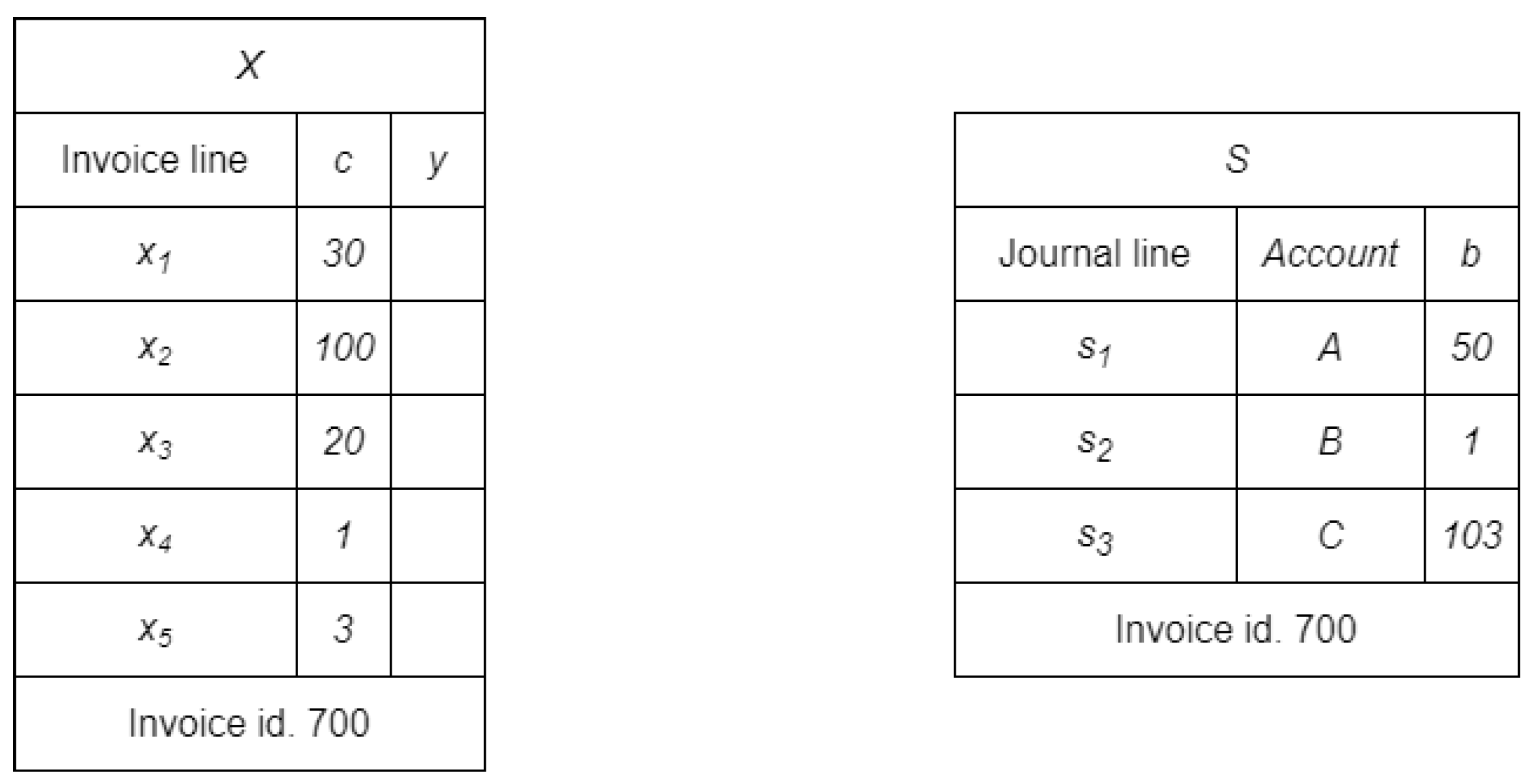
Figure 1. A toy example representing an invoice and its journal registrations before any processing.
Bdcc 07 00155 g001
Figure 2. Workflow diagram (A) describes how the problem is dealt with in a purely supervised framework. Diagram (B), on the other hand, presents the additional components in the innovative semi-supervised approach we are proposing and highlights the smaller number of discarded data.
Bdcc 07 00155 g002
Figure 3. Same example as in Figure 1 but after the label field was populated due to the resolution of the knapsack problem.
Bdcc 07 00155 g003
Figure 4. In the scheme on the left, each invoice line is assigned to the correct account via the pseudo-label and in fact the sums of the prices are matched in S. In contrast, in the scheme on the right, the second line is incorrectly classified in account A and should be changed.
Bdcc 07 00155 g004
Figure 5. Transition model: how y ^ ( n ) is transformed in y ^ ( n + 1 ) because of action C 2 . This example recalls Figure 4 and shows how one step of the search algorithm can fix the wrong situation.
Bdcc 07 00155 g005
Figure 6. Data pre-processing example: each information in an invoice line is transformed in a numerical vector and then they are concatenated in a single feature vector x.
Bdcc 07 00155 g006
Figure 7. Graph explored by A* algorithm.
Bdcc 07 00155 g007
Figure 8. Accuracy values measured over 10 folds for both the purely supervised framework and proposed one.
Bdcc 07 00155 g008
Figure 9. Same accuracy values as in Figure 8 by means of scatter plots in order to show the data distribution.
Bdcc 07 00155 g009
Table 1. Comparison of research works in accounting.
WorkComputer VisionML for EstimatesTransaction ClassificationSemi-SupervisedGraph Search
[12,13,14,15,16]
[12,17,18,19]
[6,8,20,21]
[23,24,25,26]
[27,28,29,30]
Our Proposal
Table 2. Average accuracy in three working frameworks. The percentage in bold font are the best result achieved over the compared models and frameworks.
ModelSupervised FrameworkStandard Semi-Supervised FrameworkSemi-Supervised Framework + A*
SVM89%84%90%
Naïve Bayes88%86%90%
Decision Tree88%88%92%
Random Forest91%91%93%
AdaBoost91%91%93%
Table 3. Metrics overview for Random Forest in our framework, measured with a 10-fold cross-validation.
MetricFold 1Fold 2Fold 3Fold 4Fold 5Fold 6Fold 7Fold 8Fold 9Fold 10Mean
Accuracy58%96%95%98%98%98%99%97%97%97%93%
F1 Weighted49%95%94%97%96%97%99%97%97%96%92%
F1 Macro79%97%89%88%97%96%89%86%98%94%91%
Table 4. Metrics improvement due to the coupling of the classifier with the A* graph search algorithm.
MetricSupervised FrameworkSemi-Supervised Framework + A*Improvement
Accuracy[88%, 91%][90%, 93%][+1%, +4%]
Discard Rate39%14%−25%
Supervised Data18052661+747
Disclaimer/Publisher’s Note: The statements, opinions and data contained in all publications are solely those of the individual author(s) and contributor(s) and not of MDPI and/or the editor(s). MDPI and/or the editor(s) disclaim responsibility for any injury to people or property resulting from any ideas, methods, instructions or products referred to in the content.