An Improved Link Prediction Approach for Directed Complex Networks Using Stochastic Block Modeling

Abstract

Link prediction finds the future or the missing links in a social–biological complex network such as a friendship network, citation network, or protein network. Current methods to link prediction follow the network properties, such as the node’s centrality, the number of edges, or the weights of the edges, among many others. As the properties of the networks vary, the link prediction methods also vary. These methods are inaccurate since they exploit limited information. This work presents a link prediction method based on the stochastic block model. The novelty of our approach is the three-step process to find the most-influential nodes using the m-PageRank metric, forming blocks using the global clustering coefficient and, finally, predicting the most-optimized links using maximum likelihood estimation. Through the experimental analysis of social, ecological, and biological datasets, we proved that the proposed model outperforms the existing state-of-the-art approaches to link prediction.

1. Introduction

Complex networks are used to model real-world systems such as social networks, biological entities, ecological systems, or communication networks. Citation networks, friendship networks, airline networks, mobile communication networks, and protein–protein interactions networks are a few examples of complex networks [1,2]. These systems have certain distinct characteristics. Firstly, they are very large, comprising thousands to even millions of entities. Secondly, the entities tend to interact with each other and evolve over time in ways that are difficult to predict. Thirdly, entities exhibit multiple behaviors. Lastly, entities share multiple relationships among themselves. The evolution of complex networks has been a topic of great importance since it is fundamental to correct the characterization of real-world systems. In other words, a complex network serves as a good model only to the extent that its evolution reflects the evolution of real-world systems, thereby allowing the use of the model to predict the real-world. Since the entities and their interconnections turn out to be complex in these networks, predicting the evolution of complex networks remains a challenging task. At a more fundamental level, evolution can be viewed as a series of changes within the network, wherein new entities appear, existing entities disappear, and two non-interacting existing entities start an interaction. The pace at which these changes happen also contributes to the complexity [3,4].

Graphs are fundamental data structures to represent any network. Mathematically, a graph, G = $(V,E)$, where the vertex set is denoted by V, where $V=\{v_1,v_2,\dots ,v_n\}$, and the edges are denoted by E, where $E=\{(v_i\times v_j);\{v_1,v_2,\dots ,v_n\}\in V,i\ne j\}$. The vertices represent the entities, and the edges represent the relationship between the entities. Complex networks comprise multiple subsystems, and hence, a simple graph representation is not sufficient. Consider a citation network with different kinds of entities papers, authors, citations, keywords, publication year, and several other characteristics. 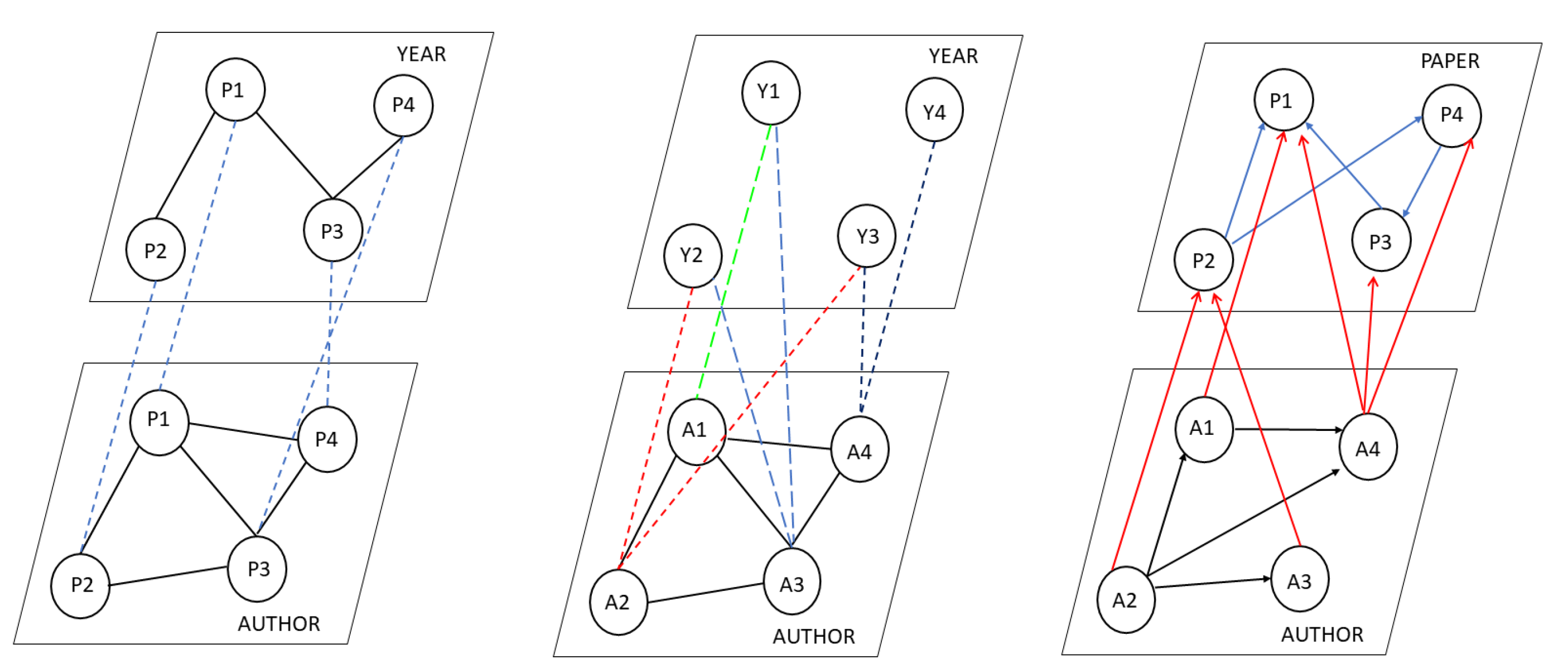Figure 1 provides three different representations of citation networks of such a network arranged hierarchically in the form of layers. For simplicity, the representations consider only a couple of characteristics. In the first representation given in Figure 1 (left), every layer consists of the same set of nodes, i.e., papers. The intra-layer links depict the relationship based on a specific aspect such as the author or publication year. For example, the link between two publications at the author layer could indicate that they share a common author. The inter-layer links depict the common aspects between the entities. It should be noted that we associate meaning with the intra- and inter-links. In the second representation given in Figure 1 (middle), each layer consists of different sets of nodes. The lower layer is the authors, and the higher layer is the publication year. Again, the meaning of intra- and inter-layer links is associated by us. Both are multilayered representations.

There needs to be more than the monoplex network representation of the objects and the relations, for instance hosting objects and relations of different scales, called multilayer networks. A multilayer network is defined as a set of nodes, edges, and layers, where the layers’ interpretation depends on the model’s implementation. Kivelä et al. [5] defined a multilayer network as a quadruple, $G_M=(V_M,E_M,V,L)$, in which the network is a collection of elementary layers $L=L_1\cup L_2\dots L_n$ stacked together. A layer is associated with a layer number and an aspect d. $V_M$ represents the set of vertices in each layer. Let $\alpha$ be a layer; the set of vertices of layer $\alpha$ is denoted as $V_{\alpha }=\{v_1^{\alpha },v_2^{\alpha },\dots ,v_n^{\alpha }\}$. The set of all vertices in the network is represented as V. Mathematically, $V_M\subseteq V\times L_1\times \dots \times L_n$. The interconnection of vertices is represented as $E_M$.

It turns out that working with directed multilayer networks requires certain additional considerations as opposed to undirected networks [6]. To appreciate this, consider the network given in Figure 1 (right). It is a directed multilayer network with two layers with the aspects being the authors and papers. The entities in the author layer denote the authors, and the entities in the paper layer denote the published paper. The links among the authors depict the author–author collaboration. A directed edge from the author layer to the paper layer depicts the paper published by the authors. The interrelationship among the papers elaborates the details of the citations. For instance, an edge from P2 to P1 means that paper P2 cites P1. The multilayer networks can represent:

• The relationship among the different nodes in the same layer;
• The relationships among the nodes that (possibly) belong to different layers;
• Each layer exhibiting a common aspect.

Complex networks, such as the WWW, airline transportation networks, and Twitter, have directed edges. The challenge in such networks is that not all nodes are reachable from a given node. Such complex networks exhibit that incoming and outgoing edges could follow different scaling laws. Studying such large-sized directed networks paves the way toward other topological structures. Detailed structural analyses of the network are crucial to obtain the out-degree distribution with a power-law behavior. The multilayer network deploys tensor algebra for representation. A multi-linear graph represents a product of two vector spaces, $V\otimes L$. It is a linear combination of $v\otimes l$, where $v\in V$ and $l\in L$:

$$\overline{a_{ij}}=\left\{\begin{array}{cc}1,\hfill & \mathrm{if}{a}_{ij}^{\alpha }=1forsome1\le \alpha \le m\hfill \\ 0,\hfill & otherwise\hfill \end{array}\right.$$

(1)

Link prediction plays a prominent role in suggesting the future or the missing links in a social–biological complex network. Link prediction also has a wide range of applications in different industries [7]. Link prediction finds its application in the domains of social networks for friend recommendation, citation networks for future citations, and the biological network for protein–protein interaction [8,9,10]. 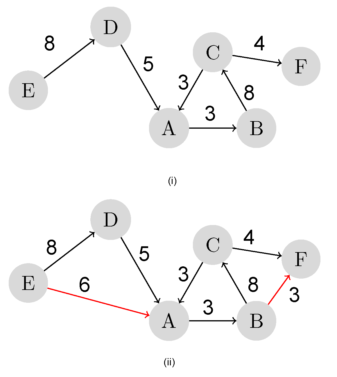Figure 2i is a snapshot of a weighted directed network, and the possible future links among the nodes are identified and established based on the least path weight, as depicted in Figure 2ii. Link prediction is an approach to detect such potential relations among individuals in social networks.

In real-time, the complex network comprises thousands of nodes. The major challenge in link prediction is retrieving the proper amount of information to perform the prediction and the enhanced algorithmic techniques to provide accurate predictions. Limitations in the availability of the attributes of the nodes redirect the link prediction algorithms to focus on the underlying network topology, which is based solely on the network structure. Most research focuses on the structural similarity indices classified as local and global.

In the local structural similarity approach, we considered the node link strengths to compute the similarity between the nodes so that they might have a link [11,12]. The local-path-based link prediction considers the structural information and the fixed distance between the nodes. The information of the nodes that lie on the set of all possible paths of a smaller length was considered [13,14]. The standard framework of link prediction methods is the similarity-based algorithm, where each pair of nodes, x and y, is assigned a score $S_{xy}$, defined as the similarity between x and y. We computed the scores between the non-observed nodes. The higher the score, the higher the likelihood of links in the future is. The local and global indices use the network properties, such as node centrality, edge count, or edge weights, among many others. Similarity measures such as the Common Neighbors (CNs) [15], Jaccard’s Coefficient (JACC), Preferential Attachment (PA) [16], Adamic–Adar index (AA) [17,18], and Cosine Similarity (CS) [19] use topological information for link prediction. As the properties of the networks vary, the link prediction methods also vary. These methods cannot be more accurate since they exploit limited information. The main drawback of local indices is that local information restricts the set of nodes’ similarity to be computed at two nodes’ distance.

Many traditional algorithms that aim to compute pairwise similarities between vertices of such a big graph need to be more accurate. Random walk utilizes a Markov chain, which describes the sequence of nodes visited by a random walker. The transition probability matrix can describe this process. Indices use the entire network’s topological information to score each link. Global indices such as the Katz index and Random Walk with Restart (RWR) can provide much more accurate predictions than the local ones. The main disadvantages of the global indices are that (i) the calculation of a global index is time-consuming, (ii) it might not be feasible for large-scale networks, and (iii) the global topological information is not available. The local and global indices are applied to undirected networks.

Extensive research is currently being carried out to overcome the drawbacks of link prediction using network structure alone. Section 2 discusses this more. New approaches utilize the statistical and probabilistic approach toward link prediction. These approaches necessitate the network structure by maximizing the likelihood of the observed structure. Then, the likelihood of any non-observed link is calculated according to the newly inferred information.

This article proposes an enhanced link prediction framework. Broadly, we considered the real-time situations of predicting the future links in the network. A link may originate in the future between two entities belonging to two different groups or block in an entire network emerging (inter-community). The term block refers to the group of nodes exhibiting a common behavior. Our framework was tailored to consider the global network structure of directed multilayered complex networks and applies a suitable probabilistic approach to predict the likelihood of the occurrence of a link. This enabled us to acquire deeper insights into the network’s organization, which cannot be gained from similarity-based algorithms. Hence, the significant contributions of this article are proposing the stochastic block modeling approach for link prediction by (i) an improvised algorithm to identify influential nodes in the directed multilayered complex network using m-PageRank, (ii) the global clustering of the influential nodes by extending the correlation to inter-layer nodes, (iii) predicting the probability of occurrence of future links in the network using the 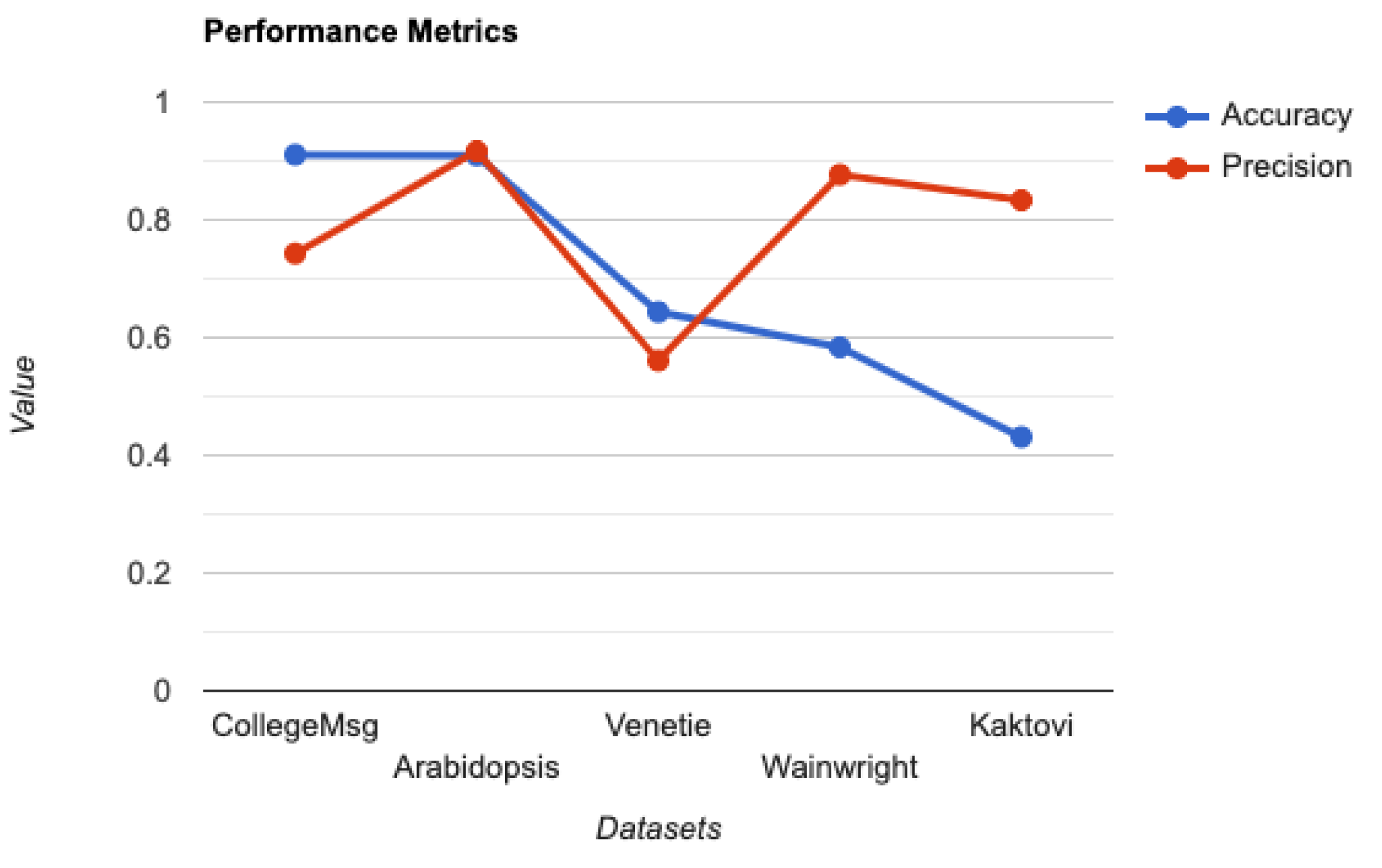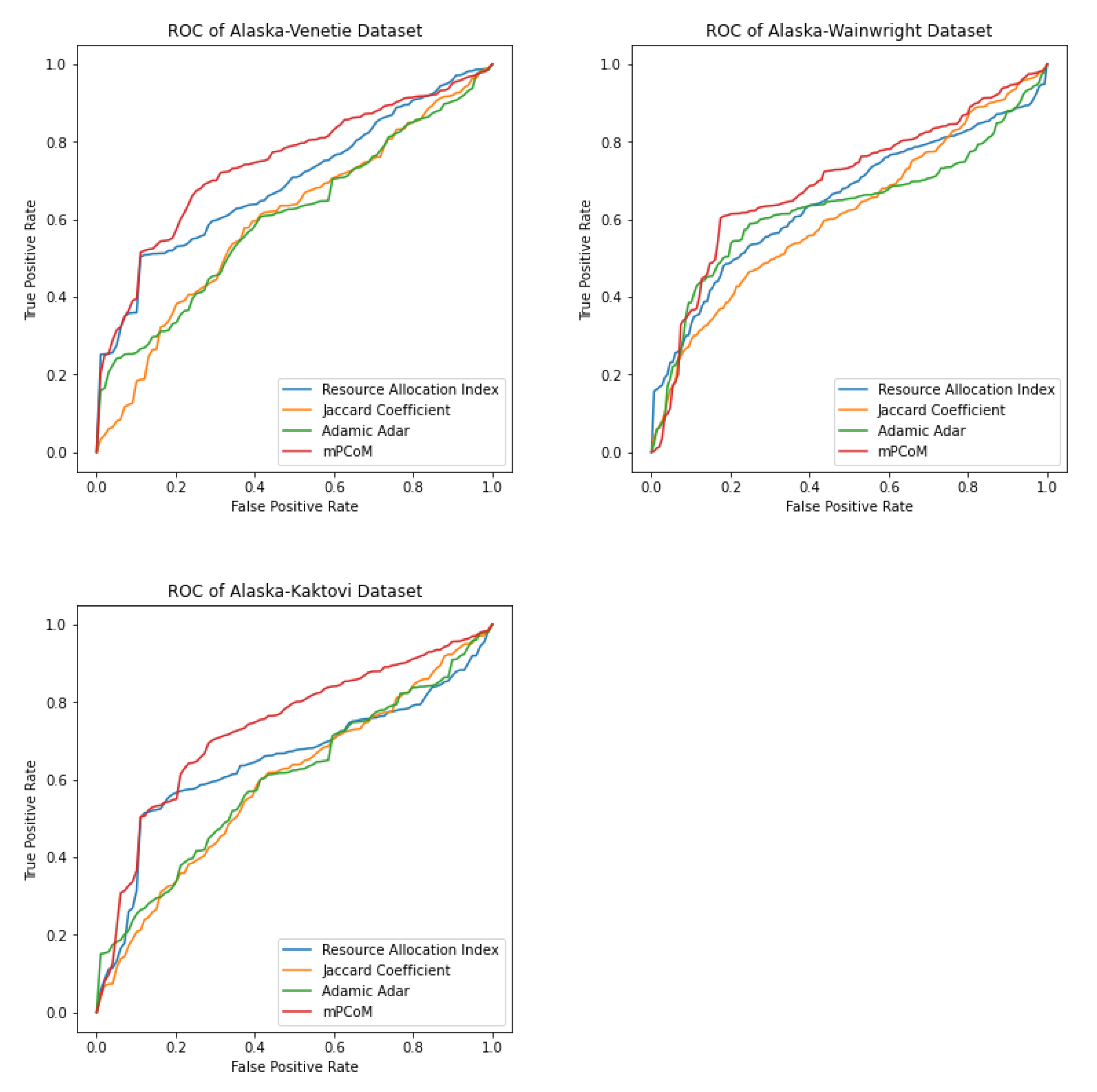maximum likelihood estimation (MLE), and (iv) empirically proving the improved accuracy and precision with social, biological, and ecological datasets. This article is organized as follows: Section 2 surveys the related work in this area. The link prediction using stochastic block modeling is illustrated in Section 3. The experimentation and implementation of the model are illustrated in Section 4. Finally, the article is concluded in Section 5.

2. Background Study

Predicting the likelihood of a link between two unconnected nodes is an interesting problem. Social network applications such as Facebook, Instagram, and Twitter require link prediction to suggest friends to a user. Link prediction also predicts missing links in a network [20,21,22].

Local indices are most suitable for undirected large-scale networks, as they consider the local information by comparing the degree of overlap among the nodes. Global indices take the properties of the whole social network into account. Random walk techniques [23,24,25,26] and PageRank techniques [27,28] are a few prominent metrics among them. On the other hand, semi-local indices omit information that makes little contribution to improving the prediction algorithm [29]. The global similarity indices depend on the amount of reachability between the nodes. Hence, the link prediction occurs only for prominent nodes and is, therefore, not wholly reliable.

In today’s era of data explosion, many large-scale social networks need to be processed and analyzed urgently, and predictions are needed based on the similarity of local nodes. Large-scale networks also demand that the algorithm be highly efficient and time-saving. The classical clustering algorithms measure local information such as Common Neighbors (CNs), the Jaccard Coefficient (JACC), and the Adamic–Adar index (AA). These algorithms mainly consider the degree or number of common neighbor nodes. The local measures such as the common neighbors, Adamic–Adar index, and resource allocation lack performance in a directed network. These algorithms are not suitable for a scale-free network. The drawbacks of local measures are:

-

The local measures based on the common neighborhood will prevent the likelihood of prediction of link establishment.

-

The local measures fail to consider the proximity of direction. Hence, prediction fails for directed graphs.

Much research has been carried out for link prediction using score-based approaches, machine learning approaches, and probabilistic approaches. Predicting the links by analyzing the topological structures of the underlying network adopts a score-based approach. This approach predicts a link by calculating the similarity score for every pair of nodes.

The researchers in [30,31] used the local main path degree index to predict the probability of a link between two nodes. The degree distribution and path strength between nodes are also used to find similarity information. In [32,33], the authors considered the entropy information of the shortest path between node pairs and proposed the Path Entropy (PE) indicator for predicting links.

The link prediction is posed as a binary classification problem. The supervised and unsupervised machine learning approaches are widely used for link prediction. In the supervised ML approach, the prediction task is carried by a classifier and uses approaches such as naïve Bayes, neural networks, decision trees, Support Vector Machine (SVM), k-nearest neighbors, bagging, boosting, and logistic regression [34,35]. On the other hand, in unsupervised machine learning, clustering techniques are used to predict the links. The probabilistic approach uses the Bayesian graphical model by considering the joint probability among the nodes in a network to predict the link. When the network sizes increase with the increase of the nodes and edges, the machine learning approach to link prediction suffers from computational complexities.

Methods such as the edge convolution operation [36], binary classification [37], and light gradient-boosted machine classification [38] approaches are adopted in deep learning models for predicting the links. To improve the link prediction performance, these deep learning models adopt more features such as the node’s interaction with neighbors, the self-degree, the out-degree, and the in-degree. Such considerations elaborate that the deep learning models also depend on the local indices. In the articles [39,40,41], the authors identified the local influencers to predict the link. The authors in [42] considered vertex ordering using the network topology information for the link predictions.

3. Stochastic Block Modeling

We propose a Stochastic Block Model (SBM) framework for solving the link prediction in directed complex networks. A block refers to a smaller group of connected nodes exhibiting a common property, which could be local or global, such as attributes and closeness. A block model or generative model refers to the collection of such blocks exhibiting some property on the data analysis performed. In the SBM, we provide a stochastic generalization of the blocks using a statistical or probabilistic approach. We formulated an estimation technique for establishing a relationship within the nodes in the network. The block model helps the distribution of the relationship between nodes. Such assumed relationships are dependent on the blocks to which the nodes belong. The relationship is established using a probabilistic estimation—the maximum likelihood estimation—to establish the relation, thereby predicting the links. It is a three-stage approach comprising:

i.

Designing an improvised algorithm to identify the influential nodes in the directed multilayered complex network using m-PageRank.

ii.

Performing global clustering of the influential nodes by extending the correlation to inter-layer nodes.

iii.

Predicting the probability of occurrence of future links in the network using the maximum likelihood estimation.

We refer to this stochastic block modeling approach as mPCoM, where mP refers to m-PageRank, Co refers to the clustering Coefficient, and M refers to the Maximum likelihood estimation. We validated the mPCoM using three different datasets from the social, biological, and ecological domains.

3.1. Identifying Influencers Using m-PageRank

An influencer in a network is a central node with more incoming edges. Influencers in the complex network help shape the network’s dynamics [43,44]. In a social network that exhibits a follower–followee relationship, the nodes may establish a relationship with a highly influential node. In a social network, the node with more incoming edges represents an influencer, since it refers to an entity (person, product, or web page) with more followers. Identifying influencers helps in various real-world tasks, such as viral marketing, epidemic outbreaks, and cascading failure. Centrality measures such as the degree, k-core, closeness, betweenness, eigenvector, and PageRank are used to identify potential influencers in complex networks.

A network or a sub-network may have one or more influencers. The nodes in a network tend to establish a link to the influencers more often than to other nodes. There needs to be more than this definition of an influencer in a multilayer network. In a multilayer network, the incoming edges of a node v can come from either the same or different layers. In the former case, v is an influencer in that layer (local influencer). In the latter case, v is an influencer globally. We focused on identifying global influencers. Furthermore, there can exist more than one influencer in a layer.

To identify the global influencer, more weight is given to an incoming edge if it comes from another layer. Furthermore, the weight of the layers differs. Since we considered a directed multilayer network, a PageRank algorithm for a multilayer network will enable us to identify the influencers. We selected the m-PageRank algorithm for this purpose [45,46]. The nodes with higher PageRank values will be the influencers. In a multilayer network, we associated a weight for the layers for computing the PageRank. The layer weight increases with an increase in active nodes. Usually, the layer weights are assumed from the ground truth of the dataset, or we assumed that, initially, all layers have equal weights.

The computation of the PageRank of a vertex $V_i$ in a multilayer network is broadly a two-phase process. (1) The PageRank of all nodes is computed considering the incoming edges from that layer only. (2) The PageRank of all nodes is re-computed by a two-step iterative process. (a) The layer weights are initialized to 1, and the PageRank of all the nodes is computed based on the layer weights and the current PageRank. (b) This PageRank is used to re-compute the layer weights. This layer weight and PageRank re-computation process is continued for all layers and nodes, respectively, until the PageRank converges. The nodes with higher ranks are higher influencers. The top influencers are picked based on the threshold specified by the user.

Now, we proceed to describe the m-PageRank computation in more detail. Initially, we establish the definitions of important terms.

Definition 1.

Let v be the node such that $v\in V$ in a network, and the PageRank of node v, $P{r}_v$, is the ratio of incoming edges of v to the total number of edges. For simplicity, we initialized the PageRank of all nodes to $\frac{1}{N}$, where N is the total number of nodes in the network.

Definition 2.

Let L represent the stack of layers in the network $G_m$ such that $L=L^1\times$ …$\times L^d$. The layer weight $L_v^l$ denotes the importance of the layer, computed by the cumulative weight of the nodes in an individual layer. We initialized the weight of all the layers to 1. The weight of the layer increases with more active nodes in the layer.

Definition 3.

The PageRank of node v in the lth layer, $P{r}_v^l$, is computed as the product of the layer weight $L_v^l$ (weight of the lth layer containing the node v) and the PageRank of v in the lth layer, $P{r}_v^l$, i.e., $\left[L_v^{l}XP{r}_v^l\right]$.

Definition 4.

We define the damping factor d, which represents the probability with the proportion of time that the vertex $v_i$ will randomly follow a vertex $v_j$. The value of the damping factor affects the convergence rate of PageRank. A low damping factor means that the relative PageRank will be determined by the PageRank received from external nodes A high damping factor will result in the node’s total PageRank growing higher. Ideally, the value of the damping factor is $0.85$.

The layers with more active nodes of a high PageRank and high in-strength are given more weights. Hence, we computed the inter-layer adjacency matrix for all V. This is again an iterative process. The adjacency matrix is computed as

$$a_{ij}^L=\sum _{j=1}^V\sum _{l=1}^L{a}_{ij}^{\left[L\right]}$$

(2)

Hence, the PageRank in a multilayer network ${\chi }_m^{\left[L\right]}\left(v\right)$ is computed iteratively considering the initial PageRank of all the vertices in the network cumulated with the product of the layer weight to the PageRank of every vertex and normalized by the damping factor. This is equated as

$${\chi }_m^{\left[L\right]}\left(v\right)=P{r}_i+(1-d)\sum _{V=1}^N\sum _{l=1}^M{a}_{ij}^{\left[L\right]}[L_j^{l_i}\times P{r}_v^l]$$

(3)

We illustrate the same with an example. Consider a multilayer network with two layers and seven nodes, as shown in Figure 3. We computed the m-PageRank for all the nodes using Equation (3). The ranking after 14 iterations is captured in

Table 1. m-PageRank computation for each node given in Figure 3.

Iteration	Node 1	Node 2	Node 3	Node 4	Node 5	Node 6	Node 7
1	0.4333	0.8533	0.15	0.567	0.789	1	0.987
2	0.1925	0.3766	0.15	0.747	0.987	1.0012	0.9899
3	0.1925	0.2768	0.15	0.435	0.989	1.0012	0.991
12	0.1925	0.27431	0.15	0.4123	0.992	1.0123	0.9934
13	0.1925	0.27431	0.15	0.390	1.003	1.1245	1.004
14	0.1955	0.27431	0.15	0.389	1.09	1.1245	1.023

. From the computation, it was observed that $Node6$ and $Node7$ have the highest PageRank. The incoming links from the above layer contributed to this.

Algorithm 1 elaborates the steps for identifying the influencers in the multilayer network.

When the m-PageRank calculations have settled down, the normalized probability distribution, which is the average m-PageRank for each node, will be $0.0\le \mathit{m}-\mathit{PageRank}\le 1.0$. The high PageRank-valued nodes above a threshold were selected as the influencers. A link is more often established from a node as an influencer.

Algorithm 1 Influencers’ identification using m-PageRank.

Input:$G=(V_M,E_M,V,L)$, $Threshold:T_p$

Output:$Influencers:I$  1: procedureinfluencer-idef(G)  2:     Initialize $P{r}_v^l\leftarrow 1,\forall {\mathrm{ł}}_i\in L,\forall v\in l$  3:     for $each{v}_i\in V_M$ do  4:         ${\chi }_m^{\left[L\right]}\left(v\right)=P{r}_i+(1-d){\sum }_{V=1}^N{\sum }_{l=1}^M{a}_{ij}^{\left[L\right]}\left[L_j^{l_i}XP{r}_v^l\right]$  5:     end for  6:     for each $l_i\in L$ do  7:         $I=I\cup \{V_j^l\parallel \forall V_j\in l,P{r}_{V_j}^l>=T_p\}$  8:     end for  9:     return I  10: end procedure

3.2. Building Blocks Using Correlation

We built the set of blocks around the influencers, I. For that, from the set of influencers, we calculated the correlation between the influencer and every pair of nodes $v\in V$ to form the blocks. This was performed using the global clustering coefficient. A clustering coefficient is a measure of the degree to which nodes in a graph tend to cluster together. At least three nodes are needed to form a cluster or block. The basic idea of forming a block is as follows.

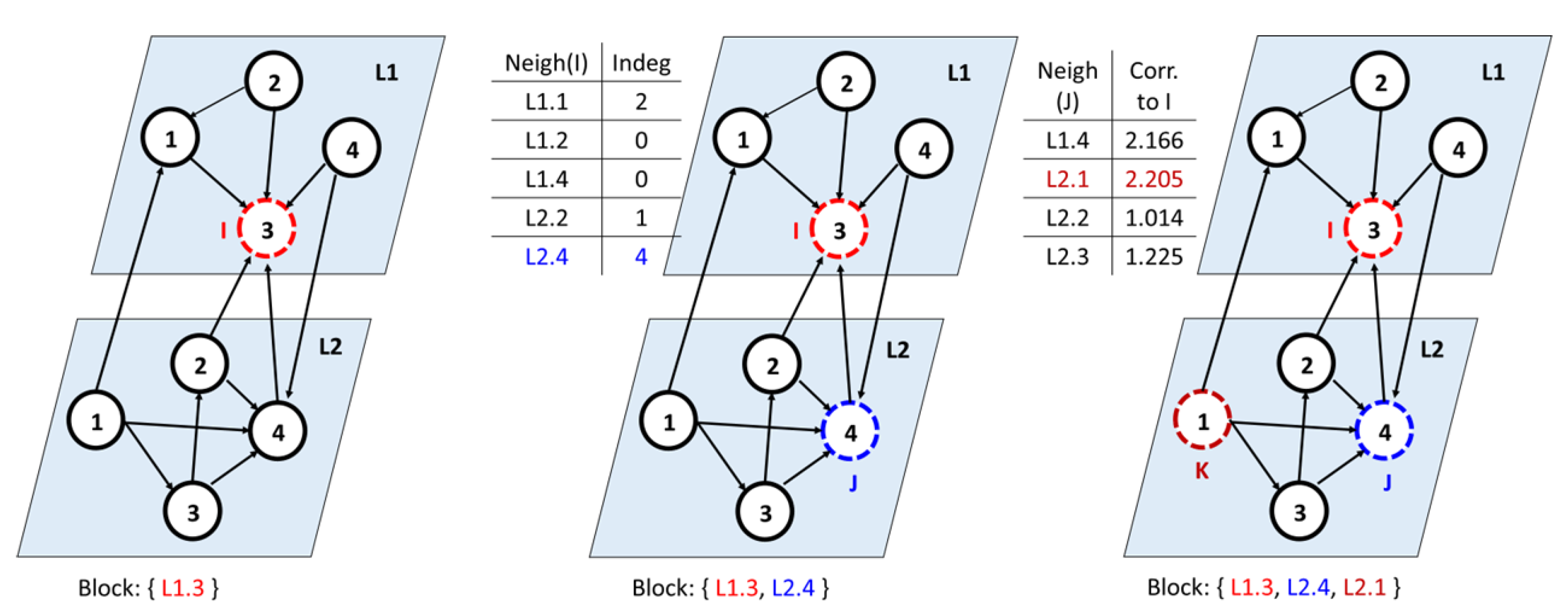
Consider the complex network with two layers, in which the nodes with the highest in-degree are an identified influencer I. Figure 4 shows an example of a multilayer network with Node 3 as the influencer from Layer 1. Among all the neighboring nodes of I, we determined a node with the highest in-degree, denoted as j. This is because in-degree(j) = 4 > in-degree($L_{1}1$). Now, j is added to I’s block. Next, for all neighbors of j, compute the correlation with I using the global clustering coefficient. To this end, we picked each neighbor k of node j and computed the correlation with I. The node k is added to the block if it has a higher correlation. Ideally, the nodes $\{I,j,k\}$ exhibit a closed triad structure, as shown in the figure. We continued with all the other influencers and constructed the blocks.

Hence, to formally define clustering coefficients in a multilayer context, we first define the triangle structure or triad structure [47].

Definition 5.

We define a triad of nodes lying up to three different layers such that the vertices in the triangles are connected by inter- or intra-layer arcs, irrespective of their orientation. This way, we can consider all possible closed triads in the inter- or intra-layer directions.

The global clustering coefficient depends on the relation between the degree of the node in the layer and the total degree of all nodes in the layer.

Definition 6.

Let L represent the stack of layers in the network $G_m$ such that $L=L^1\times$ …$\times L^d$, $D_v$ be the degree of node v, and $E_v$ represent the nodes directly connected between the neighbor nodes of node v, then the clustering coefficient, $CC\left(v\right)$, is

$$C{C}_v=\sum _{L=1}^d\frac{E_v}{\frac{D_v(D_v-1)}{2}}$$

(4)

Definition 7.

Let $S_{xy}$ be between node x and y, and let $PC\left(v\right)$ be the node centrality of v; α and β are adjustable parameters such that $\alpha +\beta =1$, $\gamma \left(v\right)$ is the set of neighbor nodes of node v, and $CC\left(v\right)$ is the clustering coefficient of v, then

$$S_{xy}=\sum _{v\in \gamma \left(x\right)\cap \gamma \left(y\right)}^{}(\alpha \frac{C{C}_v}{D_v}+\beta \frac{PC\left(x\right)PC\left(y\right)}{D_v})$$

(5)

We start by taking each influencer in its blocks and merging the highly correlated blocks. We stop the process when the desired number of clusters is formed. If the nodes in the highest correlated pair belong to different blocks, we merge these two blocks into a single one using a Merge function; otherwise, we move to the next-highest correlated pair. This process is elaborated in Algorithm 2. Thus, we obtain different blocks from the complex network. Now, we predict the links among the nodes belonging to such different blocks.

Algorithm 2 Block formation using correlation.

Input:$G=(V_M,E_M,V,L),Influencers:I$

Output: Blocks B;

1: procedureBlock formation($G,I$)  2:     Initialize $S=\{S_{xy}\parallel \forall x,y\in I,x!=y\}$  3:     $Sort\left(S\right)$  4:     for $each(x,y)\in S$ do  5:         $Merge(x,y)$  6:         return B  7:         break  8:     end for  9:  end procedure  10: procedureMerge($x,y$)  11:     if $B_x!=B_y$ then  12:         $B\leftarrow B\cup \{B_x\cup B_y\}$  13:     end if  14: end procedure

3.3. Link Prediction Using Maximum Likelihood Estimation

The identification of influencers followed by determining the blocks around them ensures both the global and local information form the basis for link prediction. The next goal is to predict the future links between pairs of blocks. To this end, we picked each pair of blocks and determined the links between the nodes of one block and the nodes of the other. Assuming n blocks, we have a total of n*(n − 1) block pairs. Among these block pairs, we determined the pair that has the highest likelihood using the maximum likelihood estimation. Let the network $G_M$ be now partitioned into multiple blocks B, such that $B=b_1\cup b_2\cup \dots b_n$. We computed the probability of the existence among two nodes a and b, such that each node belongs to a different block.

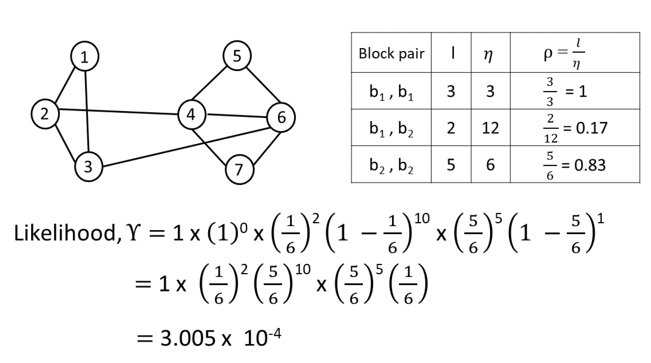
Definition 8.

Let $l_{b_1,b_2}$ be the number of edges between the nodes in the block $b_1$ and $b_2$. Assume $e_{xy}$ to be the edge between node x and node y, such that $x\in b_1$ and $y\in b_2$, and ${\eta }_{b_1,b_2}$ is the number of pairs between the nodes of blocks $b_1$, $b_2$. Then, the probability of the existence of a link between x and y is found as

$${\rho }_{b_1,b_2}=\frac{l_{b_1,b_2}}{{\eta }_{b_1,b_2}}$$

(6)

We compute the likelihood of the existence of a link, $\mathrm{{\rm Y}}$, among the blocks as:

$$\mathrm{{\rm Y}}\left(G\right|B)=\prod _{b_1,b_2\in B}{\rho }_{b_1,b_2}^{l_{b_1,b_2}}{(1-{\rho }_{b_1,b_2})}^{{\eta }_{b_1,b_2}-l_{b_1,b_2}}$$

(7)

Consider the network given in Figure 5, with two blocks. The computations of $l,\eta ,\rho ,\mathrm{{\rm Y}}$ are performed as per Equations (6) and (7). Considering all pairs of blocks, $(B,B^{\prime })$, the probability of a link with maximum likelihood $Z_{x,y}$ can be computed as:

$$Z_{x,y}=\sum _{B=1}^N\frac{\mathrm{{\rm Y}}(e_{x,y}\in E|B)\mathrm{{\rm Y}}\left(G\right|B)\rho \left(B\right)}{\mathrm{{\rm Y}}\left(G\right|B^{\prime })\rho \left(B^{\prime }\right)}$$

(8)

The higher the likelihood, the higher the probability of link formation between two nodes is. Algorithm 3 elaborates the link prediction process using the maximum likelihood estimation.

Algorithm 3 Link prediction using MLE.

Input: Blocks $B=\{b_1\cup b_2\cup \cdots b_n\}$; $B\in G_M$; nodes: $x,y$; threshold: $T_m$;

Output: probability values;

1: procedureLinkPrediction($B,x,y,T_m$)  2:     for $allxin{b}_{i}andyin{b}_j$ do  3:         $Z_{x,y}={\sum }_{B=1}^N\frac{\mathrm{{\rm Y}}(e_{x,y}\in E|B)\mathrm{{\rm Y}}\left(G\right|B)\rho \left(B\right)}{\mathrm{{\rm Y}}\left(G\right|B^{\prime })\rho \left(B^{\prime }\right)}$  4:     end for  5:     if $Z_{x,y}>=T_m$ then  6:         Return values  7:     end if  8: end procedure

4. Empirical Study

4.1. Dataset

We considered the different flavors of complex network datasets from the social, biological, and ecological real-time datasets. We considered three different datasets to establish the claimed postulates: CollegeMsg [48], Arabidopsis Genetic Layers [49], and Arctic Alaskan communities [50]. All these datasets are directed networks that are represented as multilayer networks.

4.1.1. SNAP CollegeMsg

The CollegeMsg dataset comprises private messages sent on an online social network at the University of California, Irvine. Users can search the network for others and initiate a conversation based on profile information. The initial dataset holds the information over 193 days. We constructed a multilayer network by dividing this whole period of data into ten sections.

Table 2. SNAP CollegeMsg as a multilayer network.

Layer	#Nodes	#Edges
0	699	9337
1	1183	24,181
2	1164	14,964
3	554	2279
4	472	2430
5	326	1679
6	373	1763
7	289	1407
8	249	1246
9	234	549

shows the multilayer reconstruction of the SNAP CollegeMsg dataset, the number of nodes, and the edges present in each layer.

4.1.2. Arabidopsis Multiplex GPI Network

The BIO GRID, or the Biological General Repository for Interaction Datasets, is an extensive open-source database for various organisms and species’ genetic and protein interaction data. We used the genetic interactions of Arabidopsis Thaliana. The dataset consists of seven layers. The layers are constructed from direct interaction, association, colocalization, and other genetic interactions. There are 8765 nodes and 18,655 edges over seven different layers. The details are illustrated in the

Table 3. Arabidopsis multiplex GPI network.

Layer	#Nodes	#Edges
0	5493	13,857
1	2859	4411
2	47	64
3	78	86
4	18	14
5	83	74
6	187	149

.

4.1.3. Alaska Multiplex Networks

Social and ecological structures comprise robust and critical relationships. One such network is the Arctic Alaskan communities. The network is multilayered and weighted, and the directed relationships between nodes show subsistence food flow in three sub-communities: Kaktovi, Venetie, and Wainwright. The Kaktovi multilayer consists of thirty-seven layers with twenty-thousand nodes and forty-thousand edges. The Venetie multilayer consists of forty-three layers with the same nodes and edges as Kaktovi. The Wainwright multilayer consists of thirty-six layers with thirty-seven thousand nodes and over seventy-five thousand edges. The information of the first seven layers of all three communities is shown in

Table 4. Multilayer network constructed for the Alaskan multiplex network.

	Venetie		Wainwright		Kaktovi
Layer	#Nodes	#Edges	#Nodes	#Edges	#Nodes	#Edges
0	9	236	43	1588	19	740
1	12	322	121	3900	21	696
2	23	766	117	3270	3	170
3	40	1346	44	1354	52	1606
4	5	216	131	4276	56	1560
5	69	1658	55	2128	23	594
6	5	200	76	1744	50	1658

.

4.2. Implementation and Results

4.2.1. Multilayer Network Construction

The raw datasets were not multilayered networks. In order to preserve the heterogeneous nature of the nodes in datasets, we constructed a multilayer network structure. Such multilayered networks enabled us to model a real-world system, thereby allowing us to rank the nodes. The summary of the multilayered networks constructed on various datasets is exhibited in

Table 5. Summary of multilayer networks constructed from the datasets.

Dataset	#Layers	#Nodes	#Edges
SNAP College Messages	10	8609	59,835
Arabidopsis Genetic Layers	7	8765	18,655
Alaska-Venetie	43	19,980	39,910
Alaska-Wainwright	36	37,115	75,080
Alaska-Kaktovi	37	20,071	41,258

.

4.2.2. Influential Nodes’ Identification Using m-PageRank

Our next step demanded finding the influencers in the network. The multilayered network requires the m-PageRank policy to find the influencers across the layers. These influencers contribute to meaningful correlations among the nodes in the network.

Table 6. Top five m-PageRank values identified from the constructed multilayer networks.

Coll-Msg	Arabidopsis	Venetie	Wainwright	Kaktovi
57.901003	301.720895	2.36527	6.432528	4.2054
57.835896	52.246835	2.287706	5.601206	3.373879
48.207632	50.270275	2.228333	5.066489	3.298377
41.603781	46.246756	2.160444	4.502255	3.014692
39.662304	42.390381	2.002166	4.274835	2.791716

shows us the top five influencers identified using m-PageRank in the multilayer network. Figure 6 represents a line plot of the m-PageRank of the top five influencers from the multilayered datasets.

The SNAP CollegeMSg and Arabidopsis multilayer networks exhibited a higher PageRank than the Alaskan networks. The dataset shows us the diverse connections across layers and nodes. On the other hand, in the Alaskan networks, the networks consist of robust local structures and are relatively sparse; thus, a lower PageRank was observed.

4.2.3. Formation of Blocks Using Correlation

We need to identify local structures to predict links using the stochastic block model in multilayer networks. Thus, we employed a hierarchical clustering technique using the correlation to group the influencers. We calculated the correlation between the influencers to find out how similar they are and grouped them repeatedly until the desired number of groups was formed.

Table 7. Top five correlated pairs in SNAP CollegeMsg multilayer network.

Correlation
Node A	Layer A	Node B	Layer B	Correlation
249	4	1713	4	0.502846
713	2	781	2	0.500061
298	2	298	1	0.32673
812	2	812	4	0.323473
2	0	2	1	0.320002

shows the top five correlated influencers in the multilayer network. For the experimental setup, the adjustable parameters $\alpha ,\beta$ were assigned values of $0.85$ and $0.15$, respectively.

Table 8. Blocks from SNAP CollegeMsg network.

Block Formation
BlockID	Size
42I	9
674X	9
393G	8
1282A	8
189C	8

shows the five clusters formed in the SNAP CollegeMsg multilayer network and their respective sizes.

4.2.4. Link Prediction using Maximum Likelihood Estimation

Once the clusters were formed, we predicted the possibility of future links between two influencers using a maximum likelihood estimate via stochastic block modeling.

Table 9. MLE calculated between 5 pairs of clusters in SNAP CollegeMsg multilayer network.

Maximum Likelihood Estimation
ClusterID-1	ClusterID-2	MLE
402A	400A	0.66667
402A	372A	0.166667
402A	728A	0.5
494D	429D	0.03571
494D	1189B	0.02381

shows the MLE calculated between five pairs of influencers in the SNAP CollegeMsg multilayer network. We set a threshold likelihood to predict whether a link is possible. For the performance analysis of the results, we added a new target label for the pairs. We removed 10% of the existing links labeled as positive and others as negative. Figure 7 is a line plot of the accuracy and precision observed for the multilayer networks constructed.

4.3. Results and Observations

The proposed model mPCoM was experimented on the datasets mentioned above. We used three methods for evaluating the model, namely: (i) accuracy, (ii) precision, and (iii) AUC-ROC curve. It was observed that mPCoM gave a better performance in predicting the links. The accuracy and precision obtained for each dataset are plotted in Figure 7. The proposed method mPCoM was compared with popular methods: Resource Allocation Index (RAI), Jaccard Coefficient (JACC), and Adamic–Adar index (AA).

Table 10. Comparison of accuracy of link prediction for the networks under consideration.

Accuracy
Dataset	RAI	JACC	AA	mPCoM
SNAP CollegeMSG	0.7495	0.5615	0.7350	0.742840
Alaska-Venetie	0.7245	0.7815	0.7241	0.8433
Alaska-Wainwright	0.8335	0.8166	0.8233	0.858350
Alaska-Kaktovi	0.8135	0.82114	0.80345	0.91355
Arabidopsis Multiplex GPI Network	0.6233	0.7345	0.8345	0.90123

and

Table 11. Comparison of precision of link prediction for the networks under consideration.

Precision
Dataset	RAI	JACC	AA	mPCoM
SNAP CollegeMSG	0.79495	0.73205	0.85903	0.910710
Alaska-Venetie	0.6245	0.7115	0.69941	0.866087
Alaska-Wainwright	0.73435	0.71566	0.72433	0.8767100
Alaska-Kaktovi	0.72535	0.72714	0.802415	0.88497
Arabidopsis Multiplex GPI Network	0.86733	0.77645	0.93465	0.89123

show that the proposed method had a higher accuracy and precision when compared with the existing methods. The AUC-ROC curve, as shown in Figure 8, also exhibits that mPCoM was efficient in the link prediction problem. These observations showed that the proposed mPCoM approach outperformed the state-of-the-art link prediction algorithms. Our experiments proved that the proposed approach is suitable for any directed complex network structure.

5. Conclusions and Future Work

Future link prediction is an important problem in predicting how complex networks evolve and is crucial to understanding how the network evolves. This paper proposed a stochastic block model approach for link prediction, referred to as mPCoM, which unifies the m-PageRank, correlation, and maximum likelihood estimation. We showed how the mPCoM model improves the link prediction accuracy by incorporating the global and local indices into the model. The global influencers across the network were identified based on the m-PageRank metric, which is an adaptation of the PageRank for multilayer networks. The next step focused on the formation of blocks, locally around the influencers, using global clustering, and finding the correlation between the nodes. The final step examined the block pairs and predicted the probability of a future link among the nodes of different blocks using maximum likelihood estimation. Our experiments revealed that mPCoM outperformed the state-of-the-art algorithms and gave better accuracy and precision in predicting the links. As part of future work, we propose to extend mPCoM to temporal networks, where the vertices of the complex network appear or disappear at every instance of time. This demands detailed analysis of the dynamic process of network evolution and brings in newer challenges.