A Combined System Metrics Approach to Cloud Service Reliability Using Artificial Intelligence

Abstract

Identifying and anticipating potential failures in the cloud is an effective method for increasing cloud reliability and proactive failure management. Many studies have been conducted to predict potential failure, but none have combined SMART (self-monitoring, analysis, and reporting technology) hard drive metrics with other system metrics, such as central processing unit (CPU) utilisation. Therefore, we propose a combined system metrics approach for failure prediction based on artificial intelligence to improve reliability. We tested over 100 cloud servers’ data and four artificial intelligence algorithms: random forest, gradient boosting, long short-term memory, and gated recurrent unit, and also performed correlation analysis. Our correlation analysis sheds light on the relationships that exist between system metrics and failure, and the experimental results demonstrate the advantages of combining system metrics, outperforming the state-of-the-art.

1. Introduction

Cloud computing has emerged as the fifth utility over the last decade, and is a backbone to the modern economy [1]. It is a model of computing that allows flexible use of virtual servers, massive scalability, and management services for the delivery of information services. With the low-cost pay-per-use model of on-demand computing [2], the cloud has grown massively over the years, both in terms of size and complexity.

Today, almost everyone is connected to the cloud in one way or another. This is because of cost effectiveness with a pay-as-you-go or subscription-based service model for on-demand access to IT resources [1,2]. Industries rely on the cloud for their operations, academicians to accelerate and conduct scientific experiments, and ordinary end-users by using cloud-based services knowingly or unknowingly, such as Google Drive, Gmail, Outlook, and so on. Furthermore, the cloud today is more important than yesterday, as it supports smart city construction [3], enterprise business [4], scalable data analysis [5,6], healthcare [7,8] and also new evolving computing paradigms, such as fog and edge computing [9].

To date, despite the significant improvement in the performance of the hardware elements of the cloud infrastructure, the failure rate remains substantial. Moreover, the cloud is not as reliable as the cloud service providers, such as Amazon AWS and Ali Cloud, claimed, which is more than 99.9% [10]. For example, multiple instances of failure have been reported, such as the failure of Amazon’s cloud data servers in early October 2012, which resulted in the collapse of Reddit, Airbnb, and Flipboard, the loss of Amazon AWS S3 on 28 February 2017, and the crash of Microsoft cloud services on 22 March 2017 [10]. Such failures show that cloud service providers are not as reliable as they claim [10,11].

The public cloud vendor revenue is forecast to be around 500 billion by 2026 [12]. The majority of this revenue goes to platform-as-a-service (PaaS) and infrastructure-as-a-service (IaaS), 298.4 and 126 billion, respectively. Any occurrence of the cloud’s failure, therefore, impacts the cloud-based environment and services it supports, its users, and the economy. As a result, maintaining reliability is essential, and failure prediction is one of the mechanisms to obtain it. In this study, taking advantage of the advancement in artificial intelligence (AI), we focus on failure prediction based on AI techniques of random forest (RF), gradient boosting (GB), long short-term memory (LSTM), and gated recurrent unit (GRU).

AI has the ability to learn patterns and make future predictions accordingly. AI can be manifested as a machine exhibiting human intelligence [13] and is utilised in diverse domains, such as healthcare, autonomous systems, monitoring applications, and predictive maintenance, because it allows solving problems that, before, seemed to be unsolvable by computational processes alone [14]. The tremendous advancement in AI today has resulted in state-of-the-art performance for many practical problems, especially in areas involving high-dimensional unstructured data, such as computer vision, speech, and natural language processing [15]. This ability of AI to make future predictions based on learned patterns and advancement is applied in our study.

1.1. Motivation

Today, the majority of businesses rely on cloud services to run their daily operations. Any failure of cloud services directly impacts the business, and repeated failures result in reputation damage. Reputation is an intangible asset that accounts for 85% of the value of a business [16,17]. Significant effort has been made to increase the reliability of cloud services. For failure prediction, the studies (see Section 2) either use hard drive SMART (self-monitoring, analysis and reporting technology) metrics or other system metrics, such as CPU and memory utilisation. However, despite the demonstrated ability of SMART hard drive metrics and other system metrics, such as CPU and memory utilisation to predict failures, to our knowledge, no study has combined both system metrics. We hypothesised that combining both system metrics will give us more information and, as a result, can help improve reliability further. The identified existing research gap on the combined use of SMART hard drive metrics and other system metrics, which we in our study refer to as combined system metrics, to improve reliability is the main motivation for this study. The other motivation includes the limited number of studies in the direction of server failure prediction, the use of a traditional rule-based tool, such as Prometheus [18]. Additionally, there is little, if any, correlation analysis of such metrics, which could reveal critical patterns for forecasting.

1.2. Goal

The ability to accurately predict failure is an essential factor for reliable performance. This is because it allows us to take action that is proactive. The reliability of a process depends on how well we predict failures. The aim of this study is to improve the reliability of cloud services by improving cloud server failure prediction, using selected AI techniques and the combined system metrics approach.

1.3. Contributions

Based on our motivation and goal to achieve, the main contributions of our study can be summarised as follows.

• A novel approach to server failure prediction based on combined system metrics.
• Use of AI approaches to overcome the disadvantages of rule-based failure prediction.
• A comprehensive evaluation of multiple AI techniques, such as RF, GB, LSTM and GRU, with the use of real data from more than 100 cloud servers.
• To our knowledge, this work provides the first correlation analysis (see Section 4.4) between SMART and other system metrics, such as memory utilisation.

The rest of the paper is organised as follows. In Section 2, we present a review of the state of the art. In Section 3, we present our methodology, and in Section 4 we present the performance evaluation. Finally, we conclude the paper in Section 5.

2. State-of-the-Art

In this section, we present a brief survey of recent works in failure prediction in the domain of cloud computing. Section 2.1 provides an overview of the work related to server (or server-level) failure prediction, which our work focuses on. Furthermore, we also provide a brief overview of virtual machine (VM) and task failure prediction in Section 2.2 and Section 2.3, respectively. This is to provide an overview of the research on failure prediction in the cloud domain. Finally, we provide a summary of the literature review in Section 2.4.

2.1. Server-Level Failure Prediction

Mohammed et al. [19], Xu et al. [20], Lai et al. [21], Das et al. [22], Chigurupati et al. [23], Tehrani et al. [24], and Adamu et al. [25] carried out a study on server (or server-level) failure prediction. The research by Mohammed et al. [19] focused on the prediction of containerised high-performance computing (HPC) system failures using failure information, such as hardware, software, network, undetermined, and human error. Furthermore, support vector machine (SVM), RF, k-nearest neighbours (KNN), classification and regression trees (CART), and linear discriminant analysis (LDA) were used in the study. However, we cannot tell if the system failed or if there was human intervention based on information such as human errors. Furthermore, the scope of the unidentified error source is unclear. Unlike Mohammed et al. [19], Xu et al. [20] used a ranking based machine learning approach and SMART hard drive information for failure prediction in cloud systems to improve the service availability of Microsoft Azure by migrating VMs from failing to healthy nodes.

Similar to Xu et al. [20], Das et al. [22] also focused on migrating computation from a failing node to a healthy node. However, Das et al. [22] focused on using a deep learning (i.e., LSTM) approach, compared to Xu et al. [20], who used a ranking-based approach. On the other hand, Lai et al. [21] used techniques such as KNN and hard drive data from the SLAC Accelerator Laboratory [26] to predict server failure within 60 days and introduced a derived metric time_since_prev_failure for server failure prediction. Furthermore, the study by Lai et al. [21] made use of failure logs that were kept for a period of 10 years. Based on their experience, Lai et al. [21] also recommended using an RNN-based technique, such as LSTM.

Similarly, Chigurupati et al. [23], Tehrani et al. [24], and Adamu et al. [25] used techniques such as SVM for failure prediction. While the study by Chigurupati et al. [23] focused on predicting communication hardware failure 5 min ahead, the study by Tehrani et al. [24] focused on failure prediction in cloud systems in a simulated environment, using system metrics such as temperature, CPU, RAM, and bandwidth utilisation. Adamu et al. [25], like other previous studies, focused on failure prediction in a cloud environment using data from the National Energy Research Scientific Computing Center’s [27] Computer Failure Data Repository. The author separated the failures of a disc, a dual in-line memory module (DIMM), the CPU, and other components. However, the scope of the failure, such as other failures in the study, is unclear, and network information was not used, which is another reason for the failure.

2.2. VM-Level Failure Prediction

A study on VM failure prediction was carried out by Meenakumari et al. [28], Alkasem et al. [29], Qasem et al. [30], Liu et al. [31] and Rawat et al. [32]. The study by Meenakumari et al. [28] employed a dynamic thresholding approach to predict failure based on system metrics such as CPU utilisation, CPU usage, bandwidth, temperature, and memory. Similar to Meenakumari et al. [28], Alkasem et al. [29] also focused on VM failure prediction. The study by Alkasem et al. [29] focused on the VM startup failure problem by using system metrics such as CPU utilisation, memory usage, network overhead, and IO (input/output) storage usage. Alkasem et al. [29] used Apache Spark [33] streaming together with Naïve Bayes (NB). Both Qasem et al. [30] and Liu et al. [31] investigated VM failure using recurrent neural networks (RNN). However, Qasem et al. [30] used simulated data from Cloudsim [34], whereas Liu et al. used SMART hard drive system metrics. Similar to Qasem et al. [30], Rawat et al. conducted a VM failure prediction study using simulated data. However, unlike Qasem et al. [30], Rawat et al. [32] focused on using an autoregressive integrated moving average and the Box–Jenkin method. Saxena et al. [11] proposed an online model for VM failure prediction and tolerance. The study focused on resource capacity utilisation-based failure prediction and classified virtual machines into failure-prone and normal virtual machines based on their failure tolerance units. Following the classification, the failure-prone VM was replicated into a new VM instance to be hosted on other physical machines.

2.3. Task-Level Failure Prediction

Shetty et al. [35], Jassas et al. [36], Bala et al. [37], Rosa et al. [38], Gao et al. [39], and Marahatta et al. [40] conducted a study on task failure (or job) prediction. The majority of these studies, such as Refs. [35,36,38,39], made use of the Google cluster trace dataset for their research, while the other studies, such as Refs. [37], used the simulated data from simulators such as WorkflowSim [41]. Shetty et al. [35] focused on statistical resource usage analysis as well as failure prediction using XGboost, whereas Jassas et al. [36] focused on failure analysis to identify a correlation between the failure and the requested resource. Bala et al. [37] focused on task failure prediction for scientific workflow applications, employing techniques such as NB, random forest, logistic regression (LR), and artificial neural networks (ANN).

Similar to the study of Shetty et al. [35] and Jassas et al. [36], the studies of Rosa et al. [38] and Gao et al. [39] also used the Google cluster trace dataset for their study. The study of Rosa et al. [38] also focused on job failure prediction, similar to other studies. However, unlike other studies, Rosa et al. [38] characterised failure to identify key features contributing to failure and employs techniques, such as LDA, quadratic discriminant analysis (QDA), and LR. In order to improve task failure prediction further, Gao et al. [39] proposed a multi-layer bidirectional long short-term memory (Bi-LSTM) and conducted a study, achieving an accuracy of up to 93%. Marahatta et al. [40], on the other hand, focused on energy consumption in addition to task failure prediction (i.e., energy-aware task failure prediction). Marahatta et al. [40] used deep neural networks to classify tasks (i.e., whether they are prone to failure or not) in the first stage and then scheduled them in the second stage.

2.4. Summary

We provided an overview of the related work on cloud failure prediction. Based on a review of the literature, we can see that the presented studies use system metrics, such as CPU utilisation, memory utilisation, and SMART hard drive metrics, to predict failure. However, none of the studies used those system metrics concurrently, as we did in our study, so they did not benefit from the combined use of system metrics. Using only SMART metrics, for example, excludes information from other system metrics, such as CPU utilisation, which can also be a cause of failure (i.e., which can serve as a valuable source of data for predicting failure). As such, it diminishes the potential accuracy of any failure prediction method that can otherwise be achieved using the combined use of system metrics. This phenomenon (i.e., the advantage of using multiple inputs (or metrics) over a single input) has been observed in the field of machine learning, which is a sub-field of artificial intelligence. Specifically, it was demonstrated that using multiple modality inputs (i.e., multi-modal, or in our case, multiple system inputs (or metrics)) produces more accurate predictions than using a single modality input (i.e., uni-modal, or in our case, single-system metric input) both in visual [42,43] and bio-signal analyses [44]. As a result of this discovery, we chose to use multiple system inputs (or metrics) in order to improve prediction accuracy, as we demonstrate later in the experiment results (Section 4.4.2).

3. Materials and Methods

This section details our approach. Section 3.1 contains information about data collection; Section 3.2 contains information about the data used in our study; and Section 3.3 contains information about data preprocessing. Similarly, Section 3.4, Section 3.5 and Section 3.6 discuss our implementation of RF, GB, and LSTM and GRU algorithms. Before going into detail about the implementation, Section 3.4, Section 3.5 and Section 3.6 provide an overview of the algorithms RF, GB, and LSTM and GRU, as well as the rationale for their selection.

3.1. Data Collection

There are various datasets available, including the Google job failure dataset [45], and the SMART hard drive dataset [46]. However, these datasets either contain information for job failure or hard drive failure and lack information on other system metrics, such as CPU utilisation for failure, necessitating data collection. Our data collection step entails downloading data from Prometheus [47]—monitored University of Tartu High-Performance Centre [48] cloud servers. A Python [49] script converts the downloaded JSON [50] data to CSV (Comma-separated values) format, the source code for which is available at [51].

3.2. Dataset Description

The dataset used in this study contains information about the system metrics collected through the use of Prometheus and is publicly available at [52]. The collected system metrics were chosen following a thorough assessment and analysis of their impact on the system failure.

Table 1. Selected metrics (features).

SN	Metrics	Description
1	CPU utilisation	Host CPU usage in %.
2	Memory utilisation	Memory usage in bytes
3	Network overhead	Network usage in bytes
4	IO utilisation	IO usage in time (seconds)
5	Bits read	Data written out from disk in bytes
6	Bits write	Data written into disk in bytes
7	SMART 188	Command time out
8	SMART 197	Current pending sector count
9	SMART 198	Uncorrectable sector count
10	SMART 9	Power-on hours
11	SMART 1	Read error rate
12	SMART 5	Reallocated sectors count
13	SMART 187	Reported uncorrectable errors
14	SMART 7	Seek error rate
15	SMART 3	Spin up time
16	SMART 4	Start/stop count
17	SMART 194	Temperature
18	SMART 199	UltraDMA CRC error count

summarises the selected system metrics. In addition to the selected system metrics, the dataset also contains the timestamp and anonymised server information. The dataset contains a total of 7,371,203 samples. Furthermore, details on target label generation and preprocessing are available in Section 3.3. Additionally,

Table 2. Summary of the data distribution (mean and standard deviation).

Metrics	Count/Sample Size	Mean	Std.
CPU utilisation	$\mathrm{142,706.0}$	$32.692094581900854$	$234.5717231968353$
Memory utilisation	$1.120550e+05$	$1.317217e+11$	$3.324901e+11$
Network overhead	$4.033200e+06$	$1.912711e+13$	$2.121486e+14$
IO utilisation	$7.371203e+06$	$1.922319e+05$	$6.152595e+05$
Bits read	$7.371203e+06$	$9.706407e+12$	$3.816525e+13$
Bits write	$7.371203e+06$	$3.710902e+12$	$1.555608e+13$
SMART 188	$\mathrm{19,722.0}$	$100.0$	0
SMART 197	$\mathrm{62,289.0}$	$100.0$	0
SMART 198	$\mathrm{25,372.0}$	$100.0$	0
SMART 9	$\mathrm{73,554.00}$	$93.173940$	$15.601556$
SMART 1	$\mathrm{31,005.00}$	$105.236413$	$20.515879$
SMART 5	$\mathrm{73,554.0}$	$100.0$	0
SMART 187	$\mathrm{51,027.0}$	100	0
SMART 7	$8447.00$	$89.884101$	$0.923522$
SMART 3	$8447.00$	$94.834142$	$2.034239$
SMART 4	$2814.0$	$100.0$	0
SMART 194	$\mathrm{66,529.0}$	$76.037563$	$28.240802$
SMART 199	$\mathrm{51,029.0}$	$105.514511$	$22.826553$

summarises the dataset’s statistical information in terms of mean, standard deviation (std.), and counts (or sample size). From Table 2, looking at the mean and the standard deviation, we can observe that the data are not uniformly distributed. Furthermore, Table 2 demonstrates the uneven distribution of sample sizes for various characteristics (or selected system metrics). This uneven distribution of sample sizes results in an empty value, which has an effect on the learning of machine learning algorithms. Additionally, Figure 1, Figure 2 and Figure 3 show the visualisation of the data distribution of the system metrics memory utilisation, SMART 194, and SMART 3 (selected randomly). Figure 1, Figure 2 and Figure 3 demonstrate a non-uniform data distribution as indicated by the means and standard deviations. The detailed description (or analysis) of the data is present in Section 4.4.1.

3.3. Data Preprocessing

Machine learning and, particularly, deep learning algorithms are highly dependent on data to function properly. The quality of the data affects the accuracy of the algorithm. However, the real-world data are often noisy, inconsistent and incomplete. In order to improve the result, better data are needed, or the quality of the data has to be improved. Therefore, in an attempt to improve the quality of the data, we preprocessed the data. To compensate for the missing failure information, we performed label generation as the first data preprocessing prior to any other preprocessing, as Das et al. [22], Jassas et al. [36], and Qasem et al. [53]. Algorithm 1 was utilised to generate the target label.

Table 3. Metrics and threshold used in algorithm.

SN	Metrics	Threshold
1	CPU Utilisation	>101
2	Memory Utilisation	>1,000,000,000
3	Network Overhead	> 5000
4	IO Utilisation	>16,089,590,032,253,278.0
5	Bits Read	>38,775,016,960.0
6	Bits Write	>3,189,693,620,224.0
7	SMART 188	<10
8	SMART 197	<10
9	SMART 198	<10
10	SMART 9	<10
11	SMART 1	<51
12	SMART 5	<10
13	SMART 187	<10
14	SMART 7	<10
15	SMART 3	<21
16	SMART 4	<10
17	SMART 194	>96
18	SMART 199	<10

shows the threshold value in our target label generation algorithm. The threshold was defined using information available from hardware manufacturers as well as findings from the state-of-the-art. As shown in Algorithm 1, when the value of the metrics is within the threshold, we represent it as 0; otherwise, we represent it as 1. The 0 denotes that there is no failure, whereas the 1 denotes that there is a failure. The value 0 or 1 is then appended to the list $targetValue$ via the $AppendTotargetValue$. The $targetValue$ is then used to create a new target column, which is then combined with existing data columns and returned. Further, the preprocessing techniques that handle missing values and non-standard values were employed. Missing values and non-uniform values were handled by applying the scikit-learn [54] preprocessing module.

3.4. Random Forest

Random forest (RF) is an ensemble learning method and learns using the randomised decision tree. Breiman [55] defines random forest as a classifier consisting of a collection of tree-structured classifiers $\{h(x,{\theta }_k),k=1,\dots \}$, where the $\left\{{\theta }_k\right\}$ are independent identically distributed random vectors, and each tree casts a unit vote for the most popular class at input x. The best split is chosen by optimising the classification and regression trees (CART) split criterion, which is based on the Gini impurity for classification and prediction squared error for regression [56,57].

Algorithm 1: Label generator

RF, due to its ensemble nature, provides higher accuracy and is also robust against overfitting. Furthermore, RF is capable of dealing with higher-dimensional data. RF is one of the robust general-purpose algorithms. Studies such as [56,58,59,60] have demonstrated the robustness of RF in different domains. We chose RF in our study because of its robustness against overfitting, outliers, and ability to produce better results.

In our study, we used the scikit-learn library to implement the RF algorithm [61]. The scikit-learn implementation, on the other hand, differs little from Breiman’s [55] original RF. Instead of allowing each classifier to vote for a single class, the scikit-learn implementation of RF combines classifiers by averaging their probabilistic predictions [62].

Furthermore, the scikit-learn GridSearchCV [63] was used to optimise hyperparameters, which also use the K-fold cross-validation technique to control overfitting. Data were divided into k disjoint folds of approximately equal size to the K-fold cross validation, with each fold used once as validation and the remaining k-1 fold used as training [64,65]. In our RF experiment, a value of 3 for K-fold cross validation yielded the best result.

Table 4. Random forest hyperparameter.

Parameter Name	Value
n_estimators	[100, 200, 300, 500]
max_features	[‘auto’, ‘log2’, ‘sqrt’]
criterion	[‘gini’, ‘entropy’]
min_samples_split	[3, 5, 8, 9, 10, 30, 50]

displays the selected hyperparameter and its value. Similarly,

Table 5. Tuned random forest hyperparameter.

Parameter Name	Value
n_estimators	300
max_features	‘auto’
criterion	‘gini’
min_samples_split	8

displays the optimised values for the selected RF hyperparameters after experimenting.

3.5. Gradient Boosting

Gradient boosting (GB) is another tree-based ensemble method that we used in our research due to its superior performance in a variety of domains, including medicine for predicting RNA protein interactions, flight delays, and sentiment analysis [66,67,68,69].

GB applies the boosting principle by shifting the focus to problematic observations that were difficult to predict in previous iterations and executing an ensemble of weak learners, typically decision trees [67,69]. The GB model is built iteratively, with each new model relying on the previous one. Figure 4 depicts a visualisation of the GB algorithm, learning a weak learner. The GB algorithm consists of three major components: (i) a loss function, (ii) a weak learner, and (iii) an additive model [69]. The loss function optimises the loss, which is deviance by default in scikit-learn, also known as negative log-likelihood loss [70,71]. For making predictions, the decision tree is used as a weak learner. The additive nature of the algorithm adds trees sequentially on each iteration, minimising loss.

In our study, we used the scikit-learn library to implement GB, as we did in RF. GridSearchCV was used to optimise hyperparameters in the same way that RF was used.

Table 6. Gradient boosting hyperparameter.

Parameter Name	Value
loss	[‘exponential’, ‘deviance’]
learning_rate	[0.001, 0.01, 0.0001]
max_features	[2, 3, 5, 7]
min_samples_split	[3, 4, 5, 7, 9]
n_estimators	[100, 200, 300, 500]

displays the selected hyperparameters for the GB algorithm, while

Table 7. Tuned gradient boosting hyperparameter.

Parameter Name	Value
loss	deviance
learning_rate	0.01
max_features	5
min_samples_split	3
n_estimators	500

displays the value of the optimised hyperparameter. Interestingly, similar to RF, we achieved the best results for GB using K-fold cross validation, with $k=3$.

3.6. Recurrent Neural Network

Over the years, deep learning technology has advanced significantly, outperforming cutting-edge machine learning techniques. Deep learning is now used to solve complex tasks in areas such as computer vision, autonomous systems, and climate analysis due to its performance [72]. However, the neural networks assume data independence and break with sequential data [73]. As a result, the standard neural network is incapable of accounting for temporal conditions and, thus, of making accurate predictions in situations involving sequential data, such as weather forecasting or time-series events [74]. Recurrent neural network (RNN), on the other hand, incorporates a new design architecture with hidden state or memory to account for missing dependency in standard neural networks. As a result, RNNs are preferred to conventional neural networks in situations involving temporal events. For example, Aspandi et al. [75] used LSTM, a variant of RNN, to improve facial tracking because of the involved temporal conditions. Similar to Aspandi et al. [75], our data also involve temporal events and, therefore, we use RNN in our study.

Figure 5 illustrates the RNN structure. Similarly, Equations (1) and (2) mathematically represent RNN, where U is the input weight, W is the recurrence weight, and V is the output weight. In equations, $h_t$ and $x_t$ represent the hidden vector h and the input x at time t. Tanh is a nonlinear activation function that aids in overcoming vanishing gradients, and $y_t$ is the output vector obtained by using the softmax activation function. The RNN, however, still suffers from the problem of vanishing and exploding gradients as the sequential dependency grows larger. RNN is only concerned with learning and not with selective forgetting [74]. The vanishing and exploding gradient issues occur when $\left|W\right|<1$ and $\left|W\right|>1$ or eigenvalue $\rho <1$ and $\rho >1$ for the scalar and matrix representations of the weight W, respectively [76]. The exploding gradient problem occurs when the accumulation of the gradient becomes so large that it exceeds the range. As a result, the weights become NaN and can no longer be updated. Additionally, as the gradient decays over time and becomes very small, it is overshadowed by the most recent gradient, rendering it unable to look back and remember the past efficiently.

LSTM and GRU are specialised RNN techniques that were developed specifically to address the RNN problem of vanishing and exploding gradients. As a result, our study used LSTM and GRU. Section 3.6.1 and Section 3.6.2 discuss the details of how we used LSTM and GRU.

$$h_t=tanh(W\times h_{t-1}+U\times x_t+b_h)$$

(1)

$$y_t=softmax(V\times h_t+b_v)$$

(2)

3.6.1. LSTM

Figure 6 depicts the architecture of the LSTM, and Equations (3)–(8), the computation steps involved in the LSTM [77]. The $C_t$ in Figure 6 represents the cell state, which is an additional computational unit that LSTM uses to solve the RNN problem. The other gates are input gate, output gate, and forget gate, denoted by $i_t$, $o_t$ and $f_t$, respectively. The t represents the time.

The forget gate is used to forget information, deciding whether to keep or remove information from the cell state based on the activation function sigmoid value. Tanh, on the other hand, is an activation function that is used to add nonlinearly. The output gate, which is also controlled by the sigmoid function, determines which value to take from the cell state and output. Similarly, the input gate is used to update the cell state with the new value.

$$f_t=\sigma (W_{xf}{x}_t+W_{hf}{h}_{t-1}+b_f)$$

(3)

$$i_t=\sigma (W_{xi}{x}_t+W_{hi}{h}_{t-1}+b_i)$$

(4)

$$o_t=\sigma (W_{xo}{x}_t+W_{ho}{h}_{t-1}+b_o)$$

(5)

$$C_t=f_t\odot C_{t-1}+i_t\odot tanh(W_{xc}{x}_t+W_{hc}{h}_{t-1}+b_c)$$

(6)

$$h_t=o_t\odot tanh\left(C_t\right)$$

(7)

$$Output\left(y_t\right)=softmax\left(U{h}_t\right)$$

(8)

where in the Equations (3)–(8), x denotes input, h the hidden state, W the weights, $x\ast$ (∗ denotes f, i, and o) for weight W is the input-to-hidden layer, $h\ast$ for weight W is the hidden-to-hidden layer, and U is the hidden-to-output layer weights.

Tensorflow [78] is used to implement LSTM in our study. The implemented LSTM architecture consists of eight LSTM layers and six dense layers, followed by one input and one output layer. The LSTM layer has 2048 hidden units, while the dense layer has 1024 units. Except for the output layer, each LSTM layer contains the ReLU activation function, a dropout layer with a dropout of 0.5, and L2 regularisation with a regularisation factor of 0.1. The output layer is made up of one hidden unit with a sigmoid activation. The dropout, which functions as a switch, turns off the neurons based on the provided dropout value, effectively controlling overfitting [79]. On the other hand, regularisation, such as L2 regularisation, controls the overfitting issue by penalising the model. Furthermore, we used additional overfitting control measures, such as early stopping. The use of an additional overfitting measure was driven by the observed high overfitting during the experiment. Early stopping monitors the specific metrics that were specified to be monitored and terminates training when the model begins to overfit. In our experiment, we observed validation loss. Furthermore, our implementation utilises the binary cross-entropy [80] loss function and a time shift window of length 10.

The learning rate is another critical parameter in deep learning algorithms. The learning rate indicates how far the algorithm should progress in the learning process. The learning rate is important because the model’s accuracy is determined by how well it learns. If the learning rate is too low, the learning process will become stuck in the local minima and diverge if it is too high, both of which we want to avoid. The learning rate can be set either statically or dynamically. A static learning rate value, on the other hand, would not be adaptable to changing circumstances, such as increasing or decreasing loss. As a result, in our study, we chose an adaptive learning rate to make the learning process more dynamic using the Adam optimiser [81]. We also included a learning rate scheduler to make it more dynamic. Tensorflow’s InverseTimeDecay [82] learning rate scheduler was used, with an initial learning rate of 0.001, decay steps of 2000, the decay rate of 1, and staircase False.

3.6.2. GRU

GRU is another RNN-based model that is designed to address the long-term dependency issues of RNN. GRU, like LSTM, adds new gates; however, unlike LSTM, GRU only has a reset gate $r_t$, an update gate $z_t$, and one hidden state $h_t$. The t in the reset gate, update gate, and hidden state represents time. The GRU has fewer gates and is faster than LSTM, and is often referred to as the simplified version of LSTM. Figure 7 depicts the architecture of the GRU cell, and Equations (10)–(12) represent the computational steps involved in GRU [77].

$$r_t=\sigma (W_{xr}{x}_t+W_{hr}{h}_{t-1}+b_r)$$

(9)

$$z_t=\sigma (W_{xz}{x}_t+W_{hz}{h}_{t-1}+b_z)$$

(10)

$$h_t=(1-z_t)\odot h_{t-1}+z_t\odot tanh(W_{xh}{x}_t+W_{hh}(r_t\odot h_{t-1})+b_h)$$

(11)

$$Output\left(y_t\right)=softmax\left(U{h}_t\right)$$

(12)

where in Equations (10)–(12), x denotes input, h denotes the hidden state, o denotes output, W is the weights, b is the bias, $x\ast$ (∗ represents z, r) for weight W is the input-to-hidden layer, $h\ast$ for weight W is the hidden-to-hidden layer, ⊙ is element-wise multiplication, and U is the hidden-to-output layer weights.

The reset gate r, which is similar to the LSTM forget gate, decides what to keep from the previous layer, and the update gate z decides what to move on to the next step. The reset gate and the update gate decisions are based on the sigmoid function value, as shown in Equations (9) and (10), respectively. The GRU performs the same function as the LSTM, and the reason for considering GRU is its comparable performance to the LSTM [73,74]. As a result, our GRU implementation has the same architecture as LSTM, with the exception that the LSTM layer is replaced by the GRU layer.

4. Performance Evaluation

This section details our experiment, describing how the experiment was conducted, and details how the experiment was evaluated. Section 4.1 contains the details for the experimental setup and the conduct of the experiment in Section 4.3 and the evaluation metrics that are used in Section 4.2. The data analysis and experiment results are in Section 4.4.

4.1. System Setup

The information in this section provides a complete breakdown of our system and the software used for conducting an experiment.

Computation-intensive tasks, such as the training of machine learning algorithms, require a lot of processing power. Due to this, machine learning training is almost always done using high-performance computing facilities, such as AWS (Amazon Web Service), and cloud service providers, such as Google Cloud. We have, however, in our experiment, utilised our system. Our study’s system consists of 62 GB of random access memory (RAM) with a 16 core Intel i7 3.8 GHz processor. Additionally, the system has two Nvidia RTX 2080 Ti graphics processing units (GPU). The GPU has 4352 CUDA (or Compute Unified Device Architecture) cores, with 11 GB of GDDR6 Standard Memory, and supports the Base Clock of 1350 MHz for CUDA cores and 14 Gbps memory speed and 616 GB/sec memory bandwidth [83].

The implementation can be performed using many different languages, such as Python [49], R [84] and libraries such as Tensorflow [78], Keras [85], Scikit-learn [54]. The experiment was conducted using Python [49] version 3, along with libraries such as Scikit-learn 0.22 and TensorFlow 2. The Scikit-learn library was employed in the design and implementation of the random forest classifier and gradient boosting classifier. As in the implementation of LSTM and GRU, the implementation of TensorFlow was used.

The Tensorflow is able to take advantage of the available GPU. Tensorflow, however, can be further accelerated by using TensorRT [86]. TensorRT [86] is a C++-based library provided by Nvidia that helps with high-performance inference on NVIDIA GPUs (GPUs). TensorRT is typically used to enhance and expedite the deep learning training process. Furthermore, TensorFlow includes TensorRT [86]. So, in order to use the GPU as efficiently as possible and to optimise and accelerate the deep learning training process, we also use TensorRT [86]. Our study used the TensorRT version 6.0.1. TensorRT [86] additionally needs CUDA, a parallel programming platform. In order to allow for TensorRT [86], we installed CUDA 10.0.130.

4.2. Evaluation Metrics

In this section, we go over the evaluation metrics and explain why they are necessary, as well as which evaluation metrics were chosen and why they were chosen.

Evaluation is one of the important steps of any implementation. It helps to understand the quality of implementation. In machine learning, evaluation helps to understand the model’s quality and is performed using evaluation metrics. It tells us how well the model will perform in a similar unseen scenario. Therefore, the correct use of model evaluation is vital in academic machine learning research, and many industrial settings [87].

Studies such as [88,89,90] have shown that relying on single evaluation metrics, especially in the case of unbalanced data, is not safe, as they can sometimes be misleading. Because of this reason, other studies, such as those of Das et al. [22] and Islam et al. [91], also made use of multiple evaluation metrics. Therefore, we selected multiple evaluation metrics for our work: precision, recall, accuracy, and F1 score.

4.2.1. Accuracy

Accuracy is the measure of correct overall predictions. Accuracy can be calculated by

$$Accuracy=\frac{TP+TN}{TP+TN+FP+FN}$$

(13)

where, TP is a true positive value, TN is a true negative value, FP is a false positive value and FN is a false negative value.

4.2.2. Precision

The precision, also known as positive predicted value (PPV) is a measure of a model’s exactness; a higher precision value for a classifier is preferred [88]. The precision can be calculated using Equation (14).

$$precision=\frac{TP}{TP+FP}$$

(14)

4.2.3. Recall

The recall is also called sensitivity or the true positive rate, and evaluates the classifier’s effectiveness on the positive/minority by measuring the accuracy of positive cases [88]. Recall can be calculated using Equation (15).

$$recall=\frac{TP}{TP+FN}$$

(15)

4.2.4. F1 Score

The $F1score$, also called F-measure, is the harmonic mean of precision and recall [92], and is calculated using Equation (16).

$$F1Score=2\times \frac{precision\times recall}{precision+recall}$$

(16)

4.3. Training and Testing

In this section, we describe how we trained and tested our model.

As described in Section 4.1, the system we used has two GPUs. As a result, to make the best use of the available resources and accelerate the training process, we used the distributed training strategy for LSTM and GRU. We used MirroredStrategy out of the available distributed training strategies, such as MultiWorkerMirroredStrategy, TPUStrategy, and CentralStorageStrategy [93], the reason being that the MirroredStrategy supports synchronous distributed training on multiple GPUs on one machine, and our system has both GPUs on the same machine. Further, we used the batch sizes of 556 and 430 epochs for training. Similarly, for the training of random forest and gradient boosting, we used Joblib [94] with 12 parallel jobs, using selected hyperparameters and K-fold cross validation as described in Section 3.4 and Section 3.5. Further, the details on used parameters for LSTM and GRU are presented in Section 3.6.1 and Section 3.6.2 respectively. The experiment was conducted with a 60%:40%, 55%:45%, 70%:30%, and 80%:20% train–test split. However, only the best result was recorded following the observations from studies such as those of Bala et al. [37] and Liu et al. [31], where the reported result is from only a combination of the train–test split. We obtained our results with a train–test split of 60%:40%, which is discussed in Section 4.4.2.

4.4. Results and Discussion

This section summarises our findings. In Section 4.4.1, we present the data analysis, such as an overview of the system metrics, e.g., memory usage based on the server; in Section 4.4.2, we present the experimental results and their comparison to the state-of-the-art.

4.4.1. Data Analysis

Figure 8, Figure 9 and Figure 10 depict a high-level overview of the system metrics and their usage by server. These system metrics, illustrated in Figure 8, Figure 9 and Figure 10, were chosen based on their mean and standard deviation values; three from SMART metrics and three from others system metrics. The overview of system metrics in Figure 8, Figure 9 and Figure 10 provides an analysis by the server. The analysis based on the server is taken into account in order to comprehend the server’s resource utilisation. This is because our study is devoted to predicting server failures. In all the figures, we present the hashed server information in a numeric format. This is done to aid in visualisation.

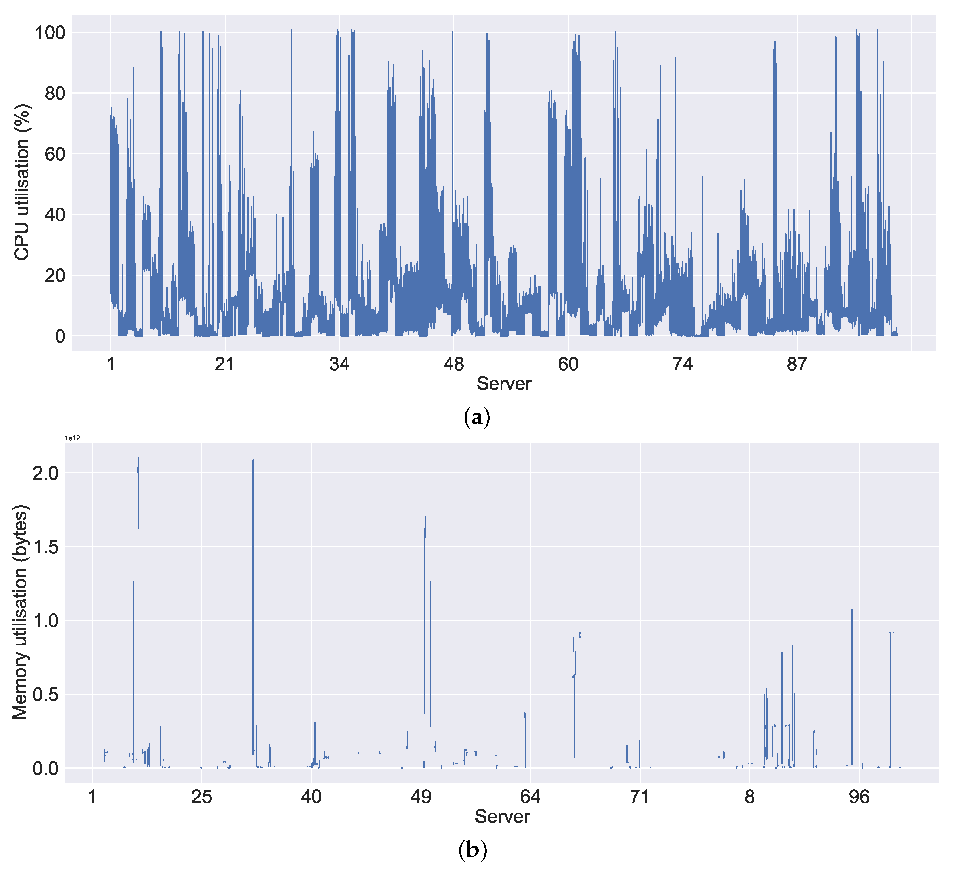
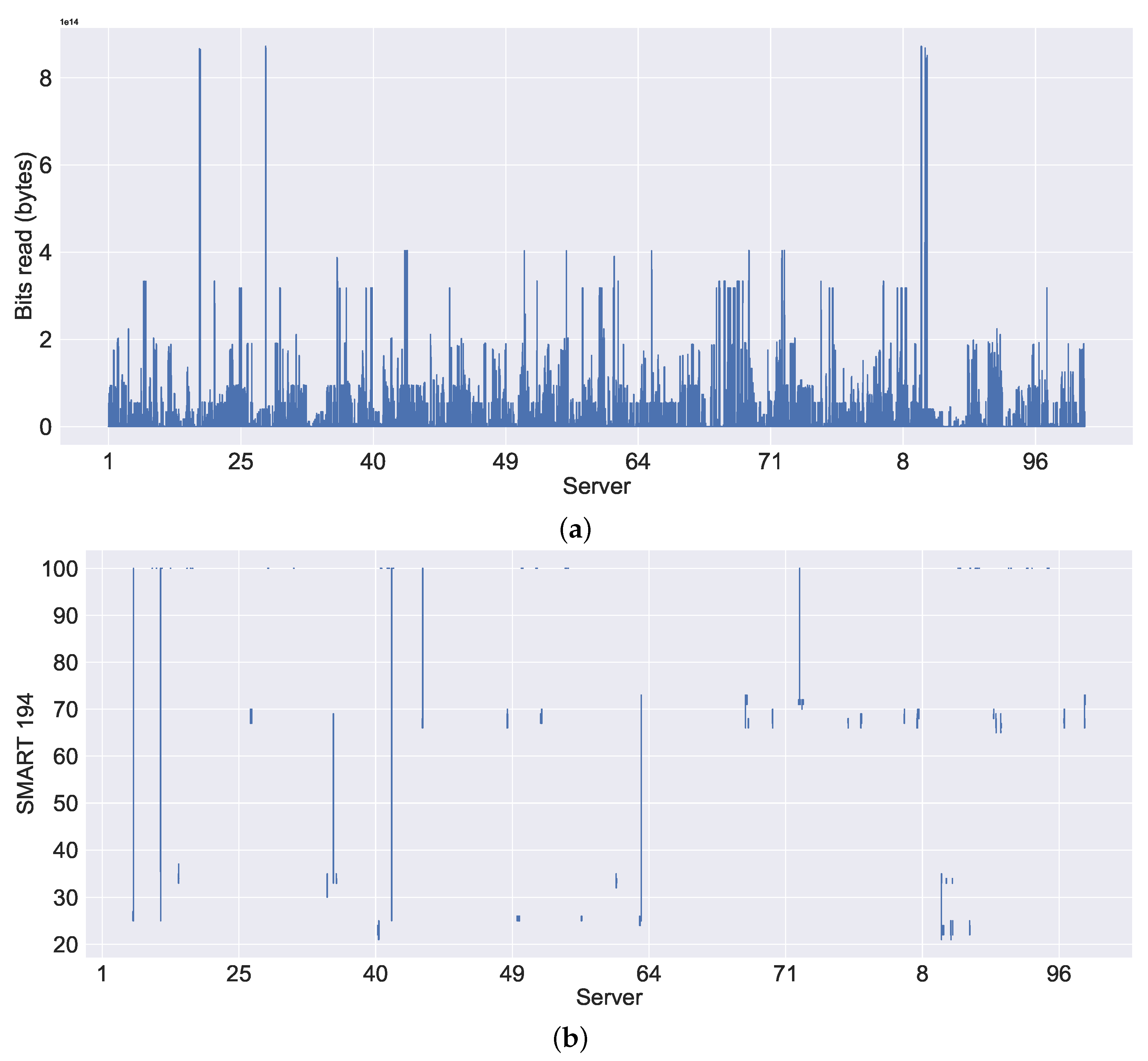
Figure 8a shows the CPU utilisation, where we considered only the CPU utilisation within the non-failure threshold (see Section 3.3). This is because of the observed high difference, which we present later in the cumulative distribution function (CDF) report. As shown in Figure 8a, we can observe the high CPU usage on all servers in general compared to the memory usage, which is shown in Figure 8b. In most cases, the servers are not making extensive use of the memory compared to the CPU. We can observe a similar pattern to that in memory usage in the system metrics bits read in Figure 9a. Moreover, we can also observe some gaps (or disconnections) in Figure 8b. This is because of the empty (or NaN) values, which could be either that the data were not available during the data collection (i.e., downloading) or that the values were missing (i.e., they were not recorded properly by the server). 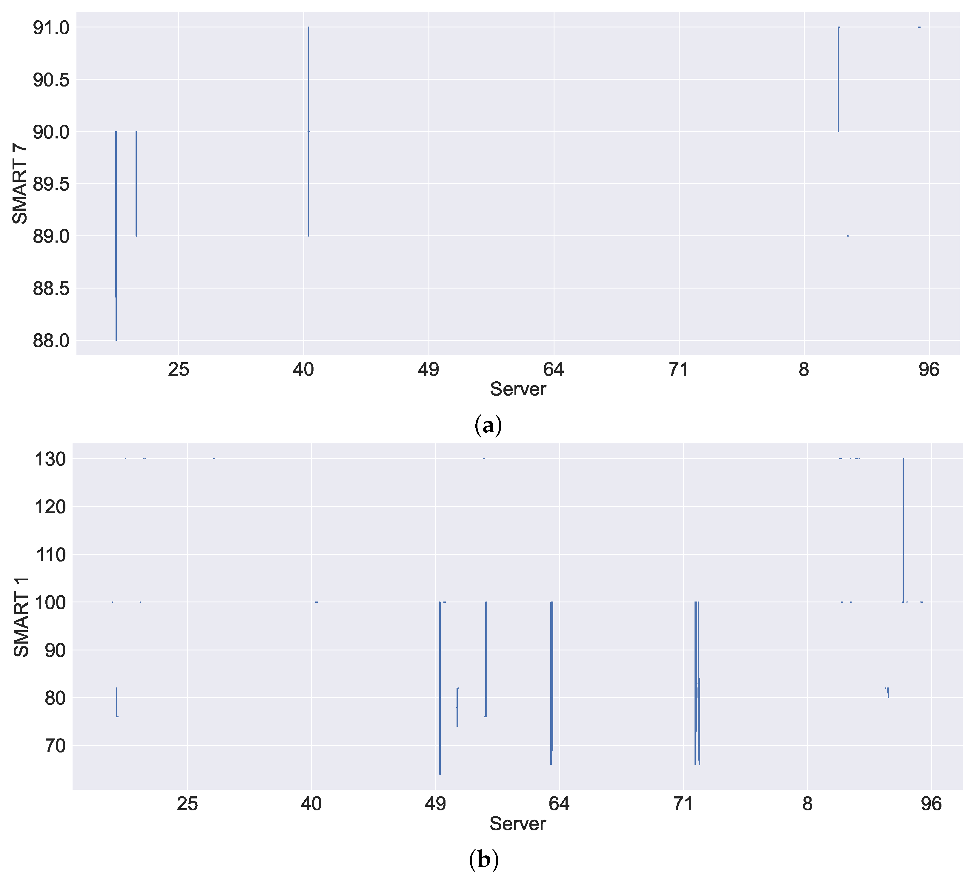Similarly, Figure 10a,b shows the visualisation of SMART 7 and SMART 1 system metrics, which monitor the state of the hard drive. In Figure 10a,b, we can observe similar patterns of disconnections to memory utilisation, resulting in NaNs.

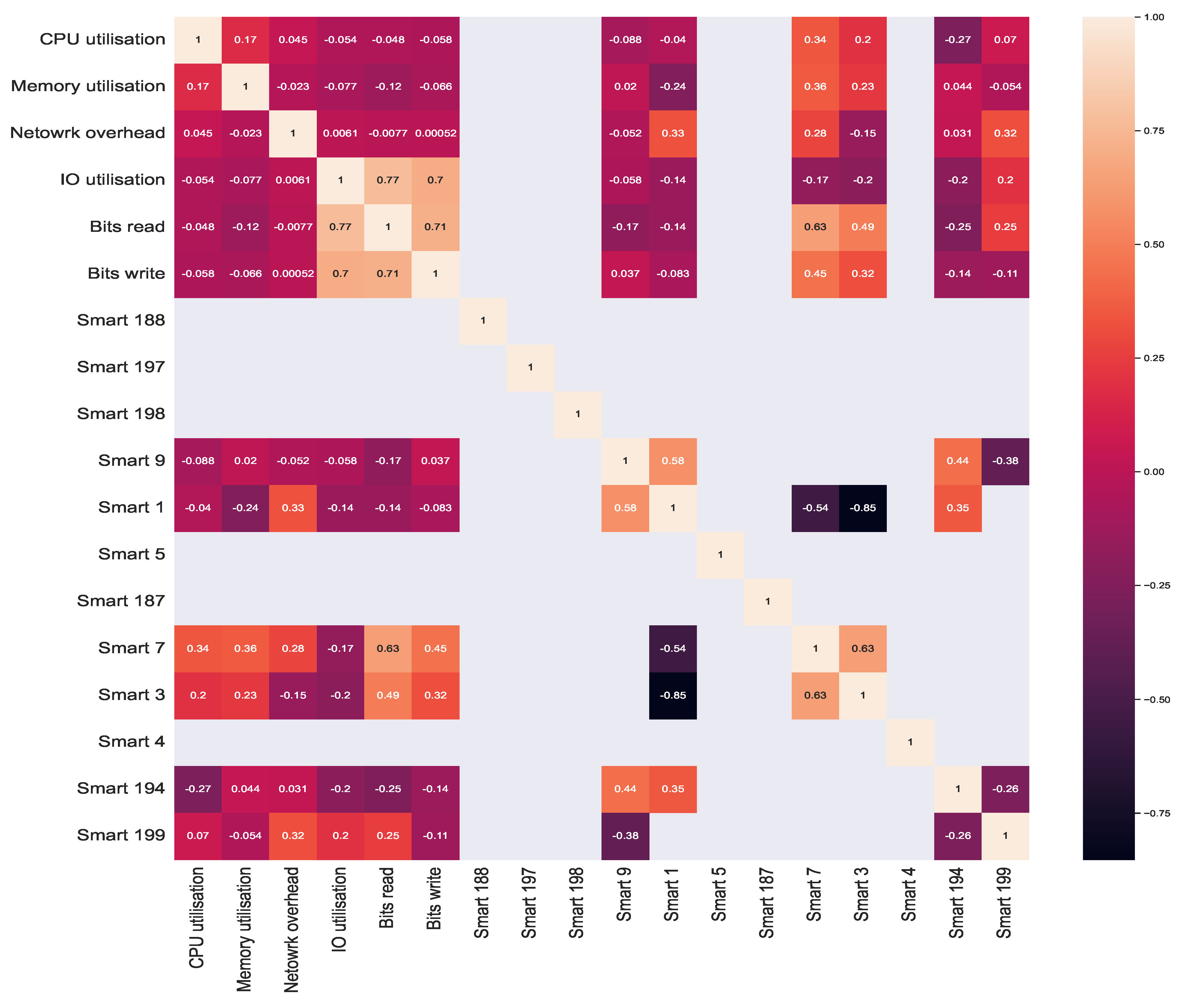
In addition, we performed a correlation analysis to better understand the relationships between the system metrics, providing for the first time a correlation analysis between the SMART system metrics and other system metrics. We used Kendall’s tau correlation coefficients for the correlation analysis. Kendall’s tau correlations for the system metrics are visualised in Figure 11. Kendall’s tau was chosen due to its mechanism of operation, which is based on comparing the rankings of values in two random variables, rather than comparing the values themselves [95]. Additionally, other correlation coefficients, such as the Pearson correlation coefficient, were not considered because they are only useful when the data are normally distributed [95]. In Figure 11, a correlation factor of 1.0 indicates a positive relationship, a factor of close to −1.0 indicates a negative relationship, and factors of 0.0 or empty values indicate that there is no correlation (i.e., no relationships).

The first observation we make is that there is a positive correlation between CPU and memory utilisation, a finding that is consistent with that of Shen et al. [96]. As with CPU and memory usage, a strong positive correlation exists between the system metrics of bits read, bits write, and IO utilisation, with a correlation factor greater than 0.7 (or 70 percent). Additionally, we observe a high correlation between the SMART 7 system metrics and other system metrics, such as bits read and bits write with a correlation factor of 0.63 for bits read and 0.45 for bits write. This relationship between SMART 7 and bits read and bits write corresponds to the functionality of SMART 7, which monitors the hard drive’s seek error rate. The other observation is that the correlations between SMART 7 and CPU and memory utilisation are also positive, with a correlation factor of 0.34 for CPU and 0.36 for memory utilisation. Similar to SMART 7, SMART 1 correlates positively with network overhead, as does SMART 3, which monitors the hard drive spin up time with bits read and bits write. Because both the bits read and bits write correspond to the hard drive, the correlation is logical, while the correlation between other SMART metrics and system metrics, such as memory utilisation, is either very low, negative, or non-existent. This observation, on the other hand, is consistent with our expectations. The reason for this is that SMART metrics track the state of the hard drive, as opposed to system metrics, such as memory usage and network overhead. In the case of SMART metrics, we can observe a high correlation between SMART 1 and SMART 9 and SMART 7 and SMART 3, with correlation factors of 0.58 and 0.63, respectively. The correlation between the remaining SMART metrics is very low or non-existent, similar to the correlation between SMART metrics and other system metrics.

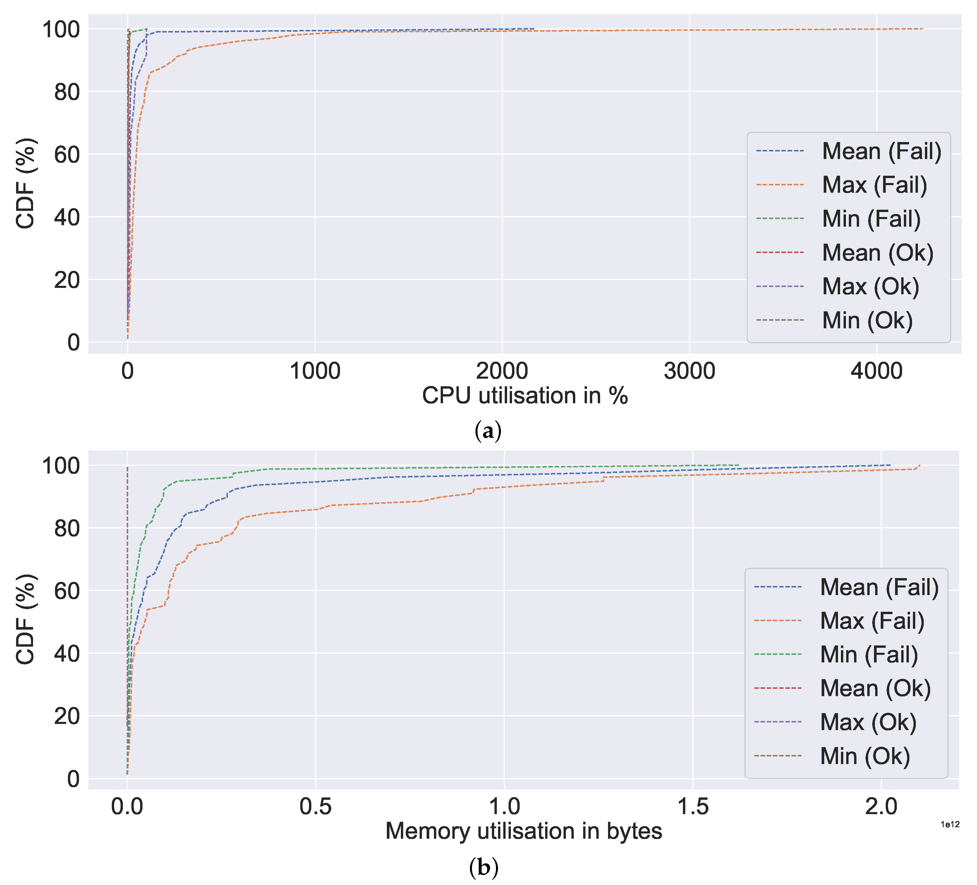
Apart from performing a correlation analysis between system metrics and generating an overview of system metrics, we also computed the CDF of the system metrics. Figure 12, Figure 13, Figure 14 and Figure 15 show the CDF visualisation of the system metrics, which were selected based on their standard deviation value (high), similar to the selection of system metrics for overview analysis. In contrast to previous analyses, such as the overview of system metrics, which focused on the server, the CDF analysis focuses on failures (or non-failures). Further, we omit system metrics with a standard deviation of zero from our CDF analysis, as this indicates that the data are centred around the mean (i.e., there is no spread). The CDF analysis summarises the mean, maximum (or max), and minimum (or min) distributions of values, which are then classified according to their failure characteristics (i.e., failure or non-failure).

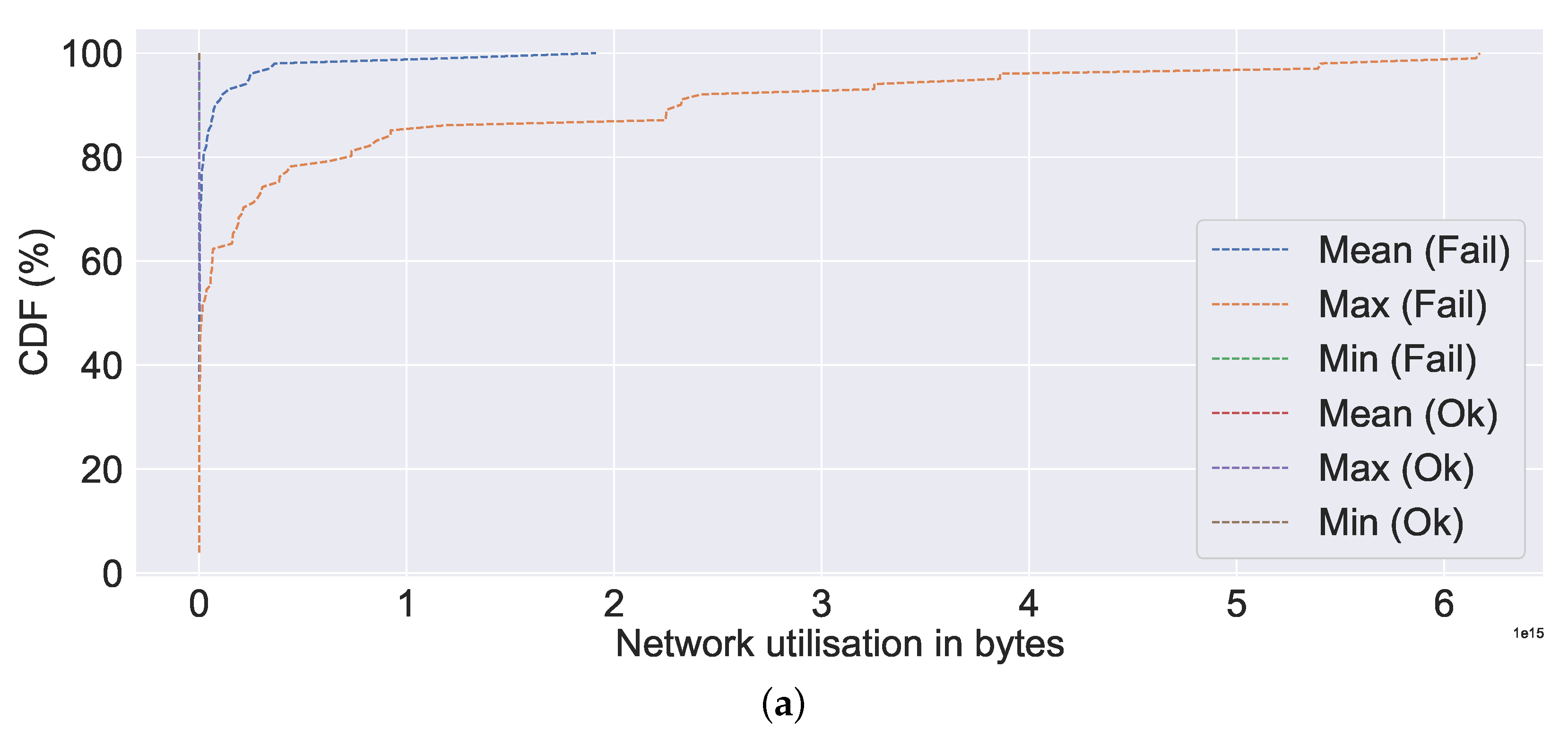
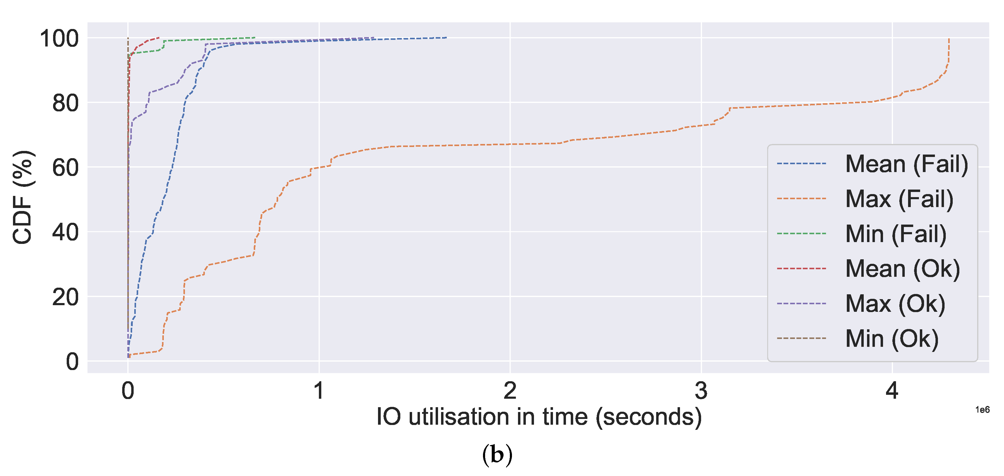
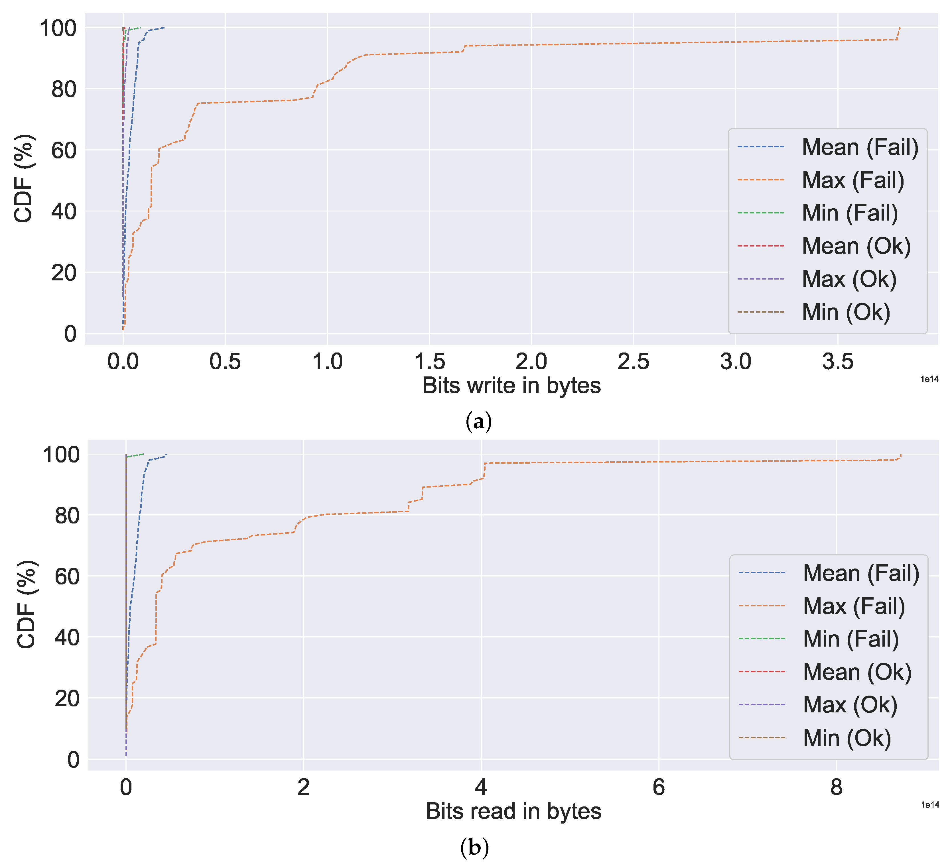
Figure 12a depicts the CPU utilisation CDF. As illustrated in Figure 12a, the mean, min, and max values for the failed server are all extremely high compared to non-failures (represented by ok in the figure). Nearly all (100% CDF) of the failed ones have very high CPU utilisation, as high as 4000%. A similar observation can be made about memory utilisation, bit write, bit read, network utilisation, and IO utilisation, all of which indicate excessive resource utilisation in the event of a failure in Figure 12b, Figure 13a,b and Figure 14a,b, respectively. Additionally, we can observe a very similar pattern for data distribution in the event of failure in the case of bits read and bits write. The abnormally high CPU utilisation value observed in our study for the failure case is consistent with the findings of Xu et al. [20], wherein in the event of a failure, a value as high as three times the normal value was observed. The observed high resource usage, such as CPU, memory, data written into and out of the disk, network usage, and increased time for IO usage in the event of failure in Figure 12, Figure 13 and Figure 14 is coherent with the failure characteristics identified by Jassas et al. [36], who observed high resource usage prior to failure. In the absence of failure, we can observe that resource utilisation is limited and relatively low. 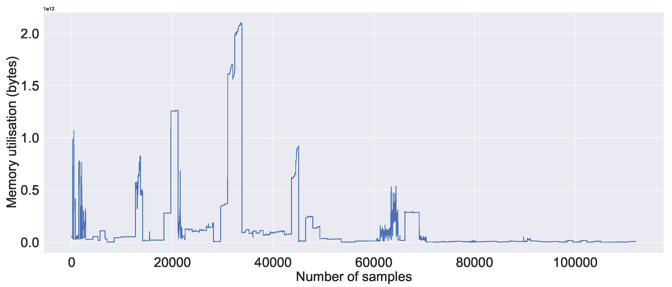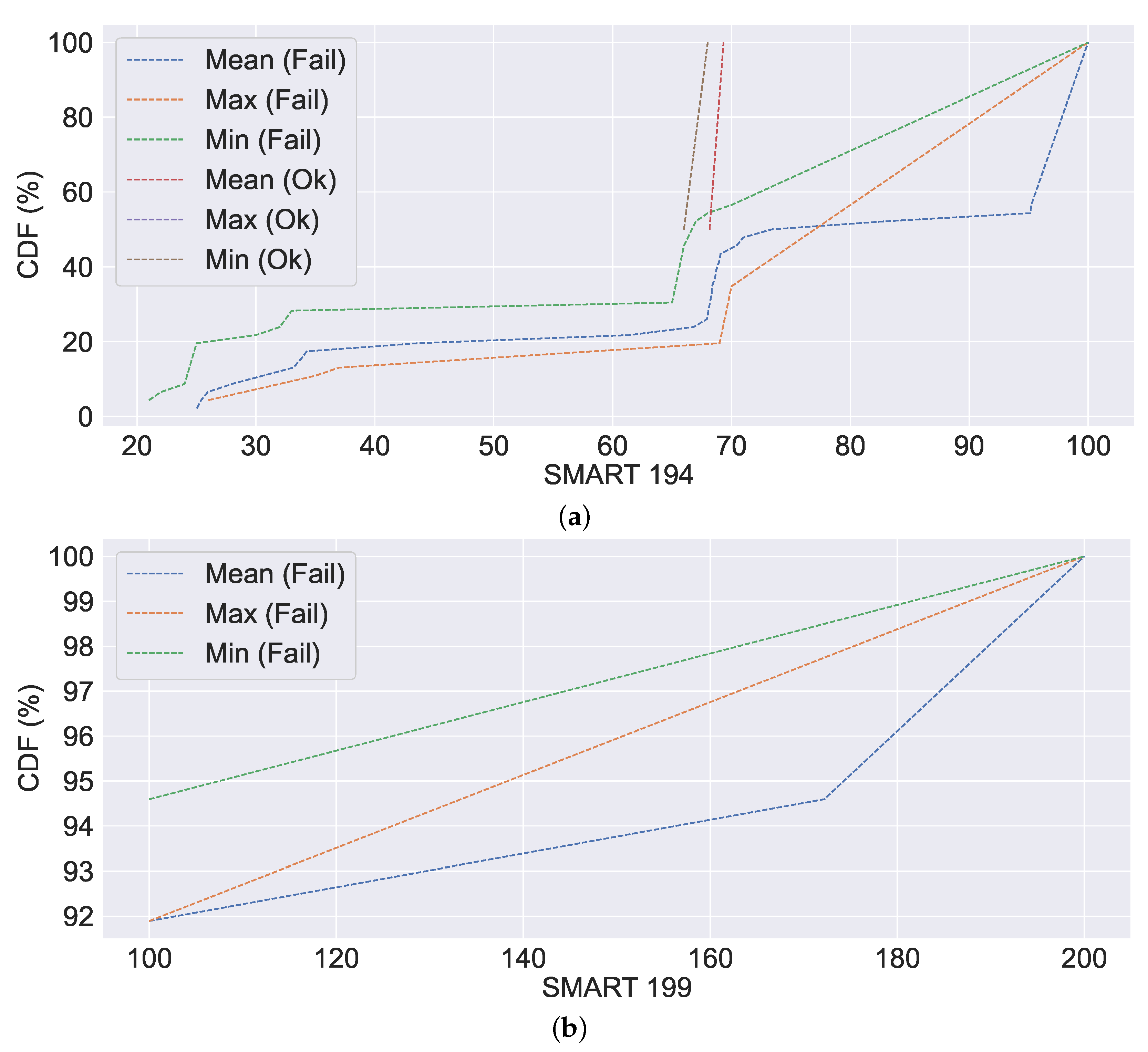The similar failure traits can also be observed in the case of the SMART system metrics from Figure 15. As illustrated in Figure 15a, the mean and min values of SMART 194 are relatively stable in non-failure cases, in contrast to the failure case, which fluctuates rapidly. Similar to SMART 194, in the case of SMART 199, we can observe high mean, min and max values in Figure 15b. Certain SMART 194 values are identical in failure to those in non-failure in Figure 15a. This is due to the failure caused by the other system metrics, where SMART metrics are reported normally. Further, we observe no CDF for SMART 199, which is not a failure. This is either because the SMART reported a failure or because other system metrics reported a failure.

We draw the following conclusions from our analysis of the data: The first conclusion is based on the overview of the server’s system metrics. We conclude that the majority of the time, resources are not fully utilised. For example, CPU utilisation is frequently less than 60%. The second is constructed using correlation analysis. Correlations between SMART system metrics and other system metrics are minimal. The third is based on an analysis of the CDF data. Resource consumption is typically high in the event of or prior to failure. Finally, the data analysis demonstrates the benefits of combining SMART metrics with other system metrics, as observed in CDF, where SMART does not report failures but other system metrics do.

4.4.2. Experimental Result

Table 8. Experimental result and its comparison to the state-of-the-art.

	Accuracy	Precision	Recall	F1 Score
Our RF	0.99	0.99	1	0.99
Our GB	0.99	0.95	1	0.97
Our LSTM	0.94	0.94	1	0.96
Our GRU	0.94	0.94	1	0.96
DESH (2018) [22]	overall 0.83 (max. 0.86)	overall 0.84 (max. 0.97)	0.87	overall 0.85 (max. 0.89)
FPHPC (2019) [19]	0.90	-	0.67	-
RTMBAS (2018) [29]	0.92	-	-	-
FACS (2019) [91]	0.91	-	-	-
PSFML (2018) [21]	-	-	-	0.94

presents our experimental results and also a comparison to the state-of-the-art. Overall, we observe high accuracy, precision, recall, and F1-score with all four of the algorithms tested, using our combined system metrics approach, with results averaging at least 95% for each algorithm. The consistent high values of all evaluation metrics with all four selected algorithms, despite the unevenly distributed data (see Section 3.2), demonstrates the benefits of the combined system metrics approach, validating our claim.

However, when we examine the results at a finer level, we can see that RF outperforms GB, LSTM, and GRU. The GB comes in second on the list, with accuracy being as close to RF as possible. The GB, on the other hand, falls short in precision by nearly 4% when compared to the RF. LSTM and GRU have comparable performance, but GB and RF outperform them by about 4–5% in terms of accuracy and precision and by about 2–3% in terms of the F1-score. In terms of recall, we can see that all four algorithms produced the same result.

In our study, RF outperformed all other algorithms evaluated. The reason for RF’s superior performance is its ability to generalise across diverse datasets with less hyperparameter tuning than techniques such as GB. A similar conclusion was made by Fernández-Delgado et al. [97] after evaluating 179 classifiers from 17 different families, such as decision trees, boosting, and other ensemble models on the whole UCI dataset [98]. Moreover, given the small difference between RF and GB performance, further hyperparameter tuning may result in improved GB performance. However, neural network-based models that can model arbitrary decision boundaries, such as RF, are more powerful when a large amount of data is available [99]. The lower performance of LSTM and GRU in our study compared to RF and GB could be attributed to data size. In the case of the larger datasets, LSTM and GRU can outperform RF because of their superior ability to learn patterns.

Furthermore, to understand where we stand in comparison to the most recent studies, we compared our findings to [19,21,22,29,91], which were chosen based on their recentness (2018 and later), relevancy, and the similarity of the evaluation metrics used. Additionally, when multiple algorithms were used in the comparison studies, we used the result from the best performing algorithm. In terms of accuracy, our combined system metrics approach outperforms others by up to 11% and recall by up to 32%, compared to the state-of-the-art studies. Similar observations can be made in terms of other evaluation metrics, such as precision and F1 score. Further, our combined system approach demonstrates competitive results by nearly 5% in terms of F1 score against state-of-the-art studies and precision by up to 10%. The studies FACS and DESH used LSTM as in our study. Based on the findings of these two studies, our proposed combined system approach continues to outperform the competition. However, when we compare our LSTM and GRU (i.e., a similar technique) results to the maximum DESH result, we see that DESH outperforms our proposed combined system metrics in terms of precision by up to 3%.

Finally, the results from our experiment and comparison to state-of-the-art studies substantiate our claim that using SMART metrics in conjunction with other system metrics, such as CPU and memory utilisation, can improve failure prediction. Furthermore, with improved failure prediction, we can detect potential failures accurately before they occur, allowing us to take proactive action and, as a result, improve reliability.

5. Conclusions

We hypothesised that combining multiple system metrics would improve failure prediction, and in this paper, we present our research on cloud server failure prediction. Additionally, we substantiated our hypothesis and demonstrated the competitive advantage of combined metrics through data analysis, a correlation study, and experimental results based on our acquired data from 100 different cloud servers. As a result of the data analysis and correlation study, we observed the following: (i) SMART system metrics have a very low, if any, correlation with other system metrics, such as CPU utilisation; (ii) in the event of a failure, high resource utilisation can be observed; and (iii) the benefits of combining system metrics. For instance, SMART system metrics do not include failure information, whereas other system metrics do (see Section 4.4.1). Subsequently, in a comparison of our automated failure prediction models, we discovered that all four AI algorithms, RF, GB, LSTM, and GRU, that utilise combined system metrics (or multi-modal inputs) outperformed the state-of-the-art studies. The highest accuracy, however, was obtained by RF methods, compared to other alternatives. Moreover, for competitive reasons, cloud providers and high-performance computing centres do not want their failures to be made public. This is also why such failure datasets are scarce, and those that exist are extremely old. Utilising such data (i.e., very old data) will not provide the necessary insights, for example, as a result of hardware (or technological) advancements. As a result, we were required to generate the target label, a procedure similar to that used in other studies (see Section 3.3). This, however, may not accurately reflect the actual failure pattern, as failures can occasionally occur abruptly, which we regard as a limitation of this study. The recent work by Chhetri et al. [100] on failure prediction, which focuses on hard drive failure prediction using knowledge graphs [101], has demonstrated even greater effectiveness. Future work will involve expanding on this approach of combining system metrics based on knowledge graphs, as described in [100], in order to achieve even greater effectiveness, as well as implementing the production method.

References

1. Buyya, R.; Srirama, S.N.; Casale, G.; Calheiros, R.; Simmhan, Y.; Varghese, B.; Gelenbe, E.; Javadi, B.; Vaquero, L.M.; Netto, M.A.; et al. A manifesto for future generation cloud computing: Research directions for the next decade. ACM Comput. Surv. (CSUR) 2018, 51, 1–38. [Google Scholar] [CrossRef] [Green Version]
2. Sahoo, P.K.; Dehury, C.K.; Veeravalli, B. LVRM: On the Design of Efficient Link Based Virtual Resource Management Algorithm for Cloud Platforms. IEEE Trans. Parallel Distrib. Syst. 2018, 29, 887–900. [Google Scholar] [CrossRef]
3. Jiang, D. The construction of smart city information system based on the Internet of Things and cloud computing. Comput. Commun. 2020, 150, 158–166. [Google Scholar] [CrossRef]
4. Saini, H.; Upadhyaya, A.; Khandelwal, M.K. Benefits of Cloud Computing for Business Enterprises: A Review. In Proceedings of the International Conference on Advancements in Computing & Management (ICACM), Jaipur, India, 13–14 April 2019. [Google Scholar]
5. Varadarajan, V.; Neelanarayanan, V.; Doyle, R.; Al-Shaikhli, I.F.; Groppe, S. Emerging Solutions in Big Data and Cloud Technologies for Mobile Networks. Mob. Netw. Appl. 2019, 24, 1015–1017. [Google Scholar] [CrossRef]
6. Langmead, B.; Nellore, A. Cloud computing for genomic data analysis and collaboration. Nat. Rev. Genet. 2018, 19, 208. [Google Scholar] [CrossRef]
7. Sahoo, P.K.; Dehury, C.K. Efficient data and CPU-intensive job scheduling algorithms for healthcare cloud. Comput. Electr. Eng. 2018, 68, 119–139. [Google Scholar] [CrossRef]
8. Liu, Y.; Zhang, L.; Yang, Y.; Zhou, L.; Ren, L.; Wang, F.; Liu, R.; Pang, Z.; Deen, M.J. A novel cloud-based framework for the elderly healthcare services using digital twin. IEEE Access 2019, 7, 49088–49101. [Google Scholar] [CrossRef]
9. Byers, C.; Zahavi, R.; Zao, J.K. The Edge Computing Advantage. 2019. Available online: https://www.iiconsortium.org/pdf/IIC_Edge_Computing_Advantages_White_Paper_2019-10-24.pdf (accessed on 25 December 2020).
10. Luo, L.; Meng, S.; Qiu, X.; Dai, Y. Improving failure tolerance in large-scale cloud computing systems. IEEE Trans. Reliab. 2019, 68, 620–632. [Google Scholar] [CrossRef]
11. Saxena, D.; Singh, A.K. OFP-TM: An online VM failure prediction and tolerance model towards high availability of cloud computing environments. J. Supercomput. 2022, 1–22. [Google Scholar] [CrossRef]
12. Gracely, B. Wikibon Research Cloud Computing (2015-2025). Available online: https://wikibon.com/wp-content/uploads/Wikibon-BGracely-Cloud-Computing-Nov-20152.pdf (accessed on 11 October 2021).
13. Huang, M.H.; Rust, R.T. Artificial intelligence in service. J. Serv. Res. 2018, 21, 155–172. [Google Scholar] [CrossRef]
14. Ropinski, T.; Archambault, D.; Chen, M.; Maciejewski, R.; Mueller, K.; Telea, A.; Wattenberg, M. How do Recent Machine Learning Advances Impact the Data Visualization Research Agenda? IEEE Vis Panel. Phoenix 2017. Available online: https://lahmesding.informatik.uni-ulm.de/api/uploads/25/vis17mlpanel.pdf (accessed on 2 January 2022).
15. Ramachandram, D.; Taylor, G.W. Deep Multimodal Learning: A Survey on Recent Advances and Trends. IEEE Signal Process. Mag. 2017, 34, 96–108. [Google Scholar] [CrossRef]
16. Protecting Intangible Assets: Preparing for a New Reality. Available online: https://assets.kpmg/content/dam/kpmg/uk/pdf/2020/08/lloyds-intangibles-6-aug-2020-.pdf (accessed on 24 October 2020).
17. Ajour El Zein, S.; Consolacion-Segura, C.; Huertas-Garcia, R. The Role of Sustainability in Brand Equity Value in the Financial Sector. Sustainability 2020, 12, 254. [Google Scholar] [CrossRef] [Green Version]
18. Turnbull, J. Monitoring with Prometheus; Turnbull Press: Brooklyn, NY, USA, 2018. [Google Scholar]
19. Mohammed, B.; Awan, I.; Ugail, H.; Younas, M. Failure prediction using machine learning in a virtualised HPC system and application. Clust. Comput. 2019, 22, 471–485. [Google Scholar] [CrossRef] [Green Version]
20. Xu, Y.; Sui, K.; Yao, R.; Zhang, H.; Lin, Q.; Dang, Y.; Li, P.; Jiang, K.; Zhang, W.; Lou, J.G.; et al. Improving service availability of cloud systems by predicting disk error. In Proceedings of the 2018 USENIX Annual Technical Conference (USENIX ATC 18), Boston, MA, USA, 11–13 July 2018; pp. 481–494. [Google Scholar]
21. Lai, B. Predicting Server Failures with Machine Learning; Technical Report; SLAC National Accelerator Lab.: Menlo Park, CA, USA, 2018. [Google Scholar]
22. Das, A.; Mueller, F.; Siegel, C.; Vishnu, A. Desh: Deep learning for system health prediction of lead times to failure in hpc. In Proceedings of the 27th International Symposium on High-Performance Parallel and Distributed Computing, Tempe, AZ, USA, 11–15 June 2018; pp. 40–51. [Google Scholar]
23. Chigurupati, A.; Thibaux, R.; Lassar, N. Predicting hardware failure using machine learning. In Proceedings of the 2016 Annual Reliability and Maintainability Symposium (RAMS), Tucson, AZ, USA, 25–28 January 2016; pp. 1–6. [Google Scholar]
24. Fadaei Tehrani, A.; Safi-Esfahani, F. A threshold sensitive failure prediction method using support vector machine. Multiagent Grid Syst. 2017, 13, 97–111. [Google Scholar] [CrossRef]
25. Adamu, H.; Mohammed, B.; Maina, A.B.; Cullen, A.; Ugail, H.; Awan, I. An Approach to Failure Prediction in a Cloud Based Environment. In Proceedings of the 2017 IEEE 5th International Conference on Future Internet of Things and Cloud (FiCloud), Prague, Czech Republic, 21–23 August 2017; pp. 191–197. [Google Scholar]
26. SLAC Accelerator Laboratory. Available online: https://www6.slac.stanford.edu (accessed on 15 October 2021).
27. National Energy Research Scientific Computing Center (NERSC). Available online: https://www.nersc.gov (accessed on 15 October 2021).
28. Meenakumari, J. Virtual Machine (VM) Earlier Failure Prediction Algorithm. Int. J. Appl. Eng. Res. 2017, 12, 9285–9289. [Google Scholar]
29. Alkasem, A.; Liu, H.; Zuo, D.; Algarash, B. Cloud computing: A model construct of real-time monitoring for big dataset analytics using apache spark. In Journal of Physics: Conference Series; IOP Publishing: Bristol, UK, 2018; Volume 933, p. 012018. [Google Scholar]
30. Qasem, G.M.; Madhu, B. Proactive fault tolerance in cloud data centers for performance efficiency. Int. J. Pure Appl. Math. 2017, 117, 325–329. [Google Scholar]
31. Liu, D.; Wang, B.; Li, P.; Stones, R.J.; Marbach, T.G.; Wang, G.; Liu, X.; Li, Z. Predicting Hard Drive Failures for Cloud Storage Systems. In Algorithms and Architectures for Parallel Processing; Wen, S., Zomaya, A., Yang, L.T., Eds.; Springer International Publishing: Cham, Switzerland, 2020; pp. 373–388. [Google Scholar]
32. Rawat, A.; Sushil, R.; Agarwal, A.; Sikander, A. A New Approach for VM Failure Prediction using Stochastic Model in Cloud. IETE J. Res. 2021, 67, 165–172. [Google Scholar] [CrossRef]
33. Apache Spark. Available online: https://spark.apache.org (accessed on 15 October 2021).
34. Cloudsim. Available online: http://www.cloudbus.org/cloudsim/ (accessed on 15 October 2021).
35. Shetty, J.; Sajjan, R.; Shobha, G. Task Resource Usage Analysis and Failure Prediction in Cloud. In Proceedings of the 2019 9th International Conference on Cloud Computing, Data Science & Engineering (Confluence), Noida, India, 10–11 January 2019; pp. 342–348. [Google Scholar]
36. Jassas, M.; Mahmoud, Q.H. Failure analysis and characterization of scheduling jobs in google cluster trace. In Proceedings of the IECON 2018—44th Annual Conference of the IEEE Industrial Electronics Society, Washington, DC, USA, 21–23 October 2018; pp. 3102–3107. [Google Scholar]
37. Bala, A.; Chana, I. Intelligent failure prediction models for scientific workflows. Expert Syst. Appl. 2015, 42, 980–989. [Google Scholar] [CrossRef]
38. Rosa, A.; Chen, L.Y.; Binder, W. Predicting and mitigating jobs failures in big data clusters. In Proceedings of the 2015 15th IEEE/ACM International Symposium on Cluster, Cloud and Grid Computing, Shenzhen, China, 4–7 May 2015; pp. 221–230. [Google Scholar]
39. Gao, J.; Wang, H.; Shen, H. Task Failure Prediction in Cloud Data Centers Using Deep Learning. In Proceedings of the 2019 IEEE International Conference on Big Data (Big Data), Los Angeles, CA, USA, 9–12 December 2019. [Google Scholar]
40. Marahatta, A.; Xin, Q.; Chi, C.; Zhang, F.; Liu, Z. PEFS: AI-driven prediction based energy-aware fault-tolerant scheduling scheme for cloud data center. IEEE Trans. Sustain. Comput. 2020, 6, 655–666. [Google Scholar] [CrossRef]
41. WorkflowSim. Available online: https://github.com/WorkflowSim/WorkflowSim-1.0 (accessed on 16 October 2021).
42. Srivastava, N.; Salakhutdinov, R.R. Multimodal learning with deep boltzmann machines. Adv. Neural Inf. Process. Syst. 2012, 2, 2222–2230. [Google Scholar]
43. Aspandi, D.; Mallol-Ragolta, A.; Schuller, B.; Binefa, X. Latent-Based Adversarial Neural Networks for Facial Affect Estimations. In Proceedings of the 2020 15th IEEE International Conference on Automatic Face and Gesture Recognition (FG 2020), Buenos Aires, Argentina, 16–20 November 2020; pp. 606–610. [Google Scholar]
44. Comas, J.; Aspandi, D.; Binefa, X. End-to-end Facial and Physiological Model for Affective Computing and Applications. In Proceedings of the 2020 15th IEEE International Conference on Automatic Face and Gesture Recognition (FG 2020), Buenos Aires, Argentina, 16–20 November 2020; pp. 93–100. [Google Scholar]
45. Google Compute Cluster Trace Data. Available online: https://github.com/google/cluster-data (accessed on 20 October 2021).
46. Backblaze Hard Drive Data and Stats. Available online: https://www.backblaze.com/b2/hard-drive-test-data.html (accessed on 20 October 2021).
47. Prometheus. Available online: https://prometheus.io/docs/introduction/overview/ (accessed on 20 October 2021).
48. University of Tartu. UT Rocket. 2018. Available online: https://share.neic.no/marketplace-public-offering/c8107e145e0d41f7a016b72825072287/ (accessed on 25 November 2021).
49. Python. Available online: https://www.python.org (accessed on 28 June 2021).
50. Introducing JSON. Available online: https://www.json.org/json-en.html (accessed on 22 October 2021).
51. Chhetri, T.; Dehury, C.K.; Lind, A.; Srirama, S.N.; Fensel, A. Code: A Combined System Metrics Approach to Cloud Service Reliability using Artificial Intelligence. 2021. Available online: https://github.com/tekrajchhetri/combined-system-metrics-to-cloud-services-reliability (accessed on 8 December 2021).
52. Dehury, C.K.; Chhetri, T.R.; Lind, A.; Srirama, S.N.; Fensel, A. HPC Cloud Traces for Better Cloud Service Reliability. 2021. Available online: https://datadoi.ee/handle/33/425 (accessed on 6 January 2022).
53. Qasem, G.M.; Madhu, B. A Classification Approach for Proactive Fault Tolerance in Cloud Data Centers. Int. J. Appl. Eng. Res. 2018, 13, 15762–15765. [Google Scholar]
54. Scikit-Learn: Machine Learning in Python. Available online: https://scikit-learn.org/stable/ (accessed on 20 June 2021).
55. Breiman, L. Random forests. Mach. Learn. 2001, 45, 5–32. [Google Scholar] [CrossRef] [Green Version]
56. Scornet, E.; Biau, G.; Vert, J.P. Consistency of random forests. Ann. Stat. 2015, 43, 1716–1741. [Google Scholar] [CrossRef]
57. Biau, G.; Scornet, E. A random forest guided tour. Test 2016, 25, 197–227. [Google Scholar] [CrossRef] [Green Version]
58. Kulkarni, A.D.; Lowe, B. Random forest algorithm for land cover classification. Int. J. Recent Innov. Trends Comput. Commun. 2016, 4, 58–63. [Google Scholar]
59. Ramo, R.; Chuvieco, E. Developing a random forest algorithm for MODIS global burned area classification. Remote Sens. 2017, 9, 1193. [Google Scholar] [CrossRef] [Green Version]
60. Khaidem, L.; Saha, S.; Dey, S.R. Predicting the direction of stock market prices using random forest. arXiv 2016, arXiv:1605.00003. [Google Scholar]
61. Scikit-Learn: Random Forest Classifier. Available online: https://scikit-learn.org/stable/modules/generated/sklearn.ensemble.RandomForestClassifier.html (accessed on 20 June 2021).
62. Forests of Randomized Trees. Available online: https://scikit-learn.org/stable/modules/ensemble.html#forest (accessed on 21 June 2021).
63. GridSearchCV. Available online: https://scikit-learn.org/stable/modules/generated/sklearn.model_selection.GridSearchCV.html (accessed on 21 June 2021).
64. Berrar, D. Cross-validation. In Encyclopedia of Bioinformatics and Computational Biology; Elsevier: Amsterdam, The Netherlands, 2019; pp. 542–545. [Google Scholar]
65. Wong, T.T. Performance evaluation of classification algorithms by k-fold and leave-one-out cross validation. Pattern Recognit. 2015, 48, 2839–2846. [Google Scholar] [CrossRef]
66. Athanasiou, V.; Maragoudakis, M. A novel, gradient boosting framework for sentiment analysis in languages where NLP resources are not plentiful: A case study for modern Greek. Algorithms 2017, 10, 34. [Google Scholar] [CrossRef]
67. Dangeti, P. Statistics for Machine Learning; Packt Publishing: Birmingham, UK, 2017. [Google Scholar]
68. Chakrabarty, N.; Kundu, T.; Dandapat, S.; Sarkar, A.; Kole, D.K. Flight Arrival Delay Prediction Using Gradient Boosting Classifier. In Emerging Technologies in Data Mining and Information Security; Springer: Berlin/Heidelberg, Germany, 2019; pp. 651–659. [Google Scholar]
69. Yu, A.; Chung, C.; Yim, A. Numerical Computing with Python; Packt Publishing: Birmingham, UK, 2018. [Google Scholar]
70. GradientBoostingClassifier. Available online: https://scikit-learn.org/stable/modules/generated/sklearn.ensemble.GradientBoostingClassifier.html (accessed on 21 June 2021).
71. Ensemble Methods. Available online: https://scikit-learn.org/stable/modules/ensemble.html (accessed on 21 June 2021).
72. Kurth, T.; Treichler, S.; Romero, J.; Mudigonda, M.; Luehr, N.; Phillips, E.; Mahesh, A.; Matheson, M.; Deslippe, J.; Fatica, M.; et al. Exascale deep learning for climate analytics. In Proceedings of the SC18: International Conference for High Performance Computing, Networking, Storage and Analysis, Dallas, TX, USA, 11–16 November 2018; pp. 649–660. [Google Scholar]
73. Sujit Pal, A.G. Deep Learning with Keras; Packt Publishing: Birmingham, UK, 2017. [Google Scholar]
74. Fandango, A.; Rajalingappaa, S.; Bonaccorso, G. Python: Advanced Guide to Artificial Intelligence; Packt Publishing: Birmingham, UK, 2018. [Google Scholar]
75. Aspandi, D.; Martinez, O.; Sukno, F.; Binefa, X. Fully End-to-End Composite Recurrent Convolution Network for Deformable Facial Tracking In The Wild. In Proceedings of the 2019 14th IEEE International Conference on Automatic Face Gesture Recognition (FG 2019), Lille, France, 14–18 May 2019; pp. 1–8. [Google Scholar]
76. Vasilev, I. Advanced Deep Learning with Python; Packt Publishing: Birmingham, UK, 2019. [Google Scholar]
77. Ravichandiran, S. Hands-On Deep Learning Algorithms with Python; Packt Publishing: Birmingham, UK, 2019. [Google Scholar]
78. Tensorflow. Available online: https://www.tensorflow.org (accessed on 23 June 2021).
79. Gal, Y.; Ghahramani, Z. A theoretically grounded application of dropout in recurrent neural networks. In Advances in Neural Information Processing Systems; Curran Associates, Inc.: New York, NY, USA, 2016; pp. 1019–1027. [Google Scholar]
80. BinaryCrossentropy. Available online: https://www.tensorflow.org/api_docs/python/tf/keras/losses/BinaryCrossentropy (accessed on 23 June 2021).
81. Optimizers (Adam). Available online: https://www.tensorflow.org/api_docs/python/tf/keras/optimizers/Adam (accessed on 23 June 2021).
82. Inverse Time Decay Learning Rate Schedule. Available online: https://www.tensorflow.org/api_docs/python/tf/keras/optimizers/schedules/InverseTimeDecay (accessed on 23 June 2021).
83. GEFORCE RTX 20 SERIES. Available online: https://www.nvidia.com/en-eu/geforce/graphics-cards/rtx-2080-ti/ (accessed on 28 June 2021).
84. R. Available online: https://www.r-project.org (accessed on 28 June 2021).
85. Keras. Available online: https://keras.io (accessed on 28 June 2021).
86. NVIDIA TensorRT Developer Guide. Available online: https://docs.nvidia.com/deeplearning/sdk/tensorrt-developer-guide/index.html (accessed on 28 June 2021).
87. Raschka, S. Model evaluation, model selection, and algorithm selection in machine learning. arXiv 2018, arXiv:1811.12808. [Google Scholar]
88. Akosa, J. Predictive accuracy: A misleading performance measure for highly imbalanced data. In Proceedings of the SAS Global Forum, Orlando, FL, USA, 2–5 April 2017; pp. 2–5. [Google Scholar]
89. Juba, B.; Le, H.S. Precision-recall versus accuracy and the role of large data sets. In Proceedings of the AAAI Conference on Artificial Intelligence, Honolulu, HI, USA, 27 January–1 February 2019; Volume 33, pp. 4039–4048. [Google Scholar]
90. Hossin, M.; Sulaiman, M. A review on evaluation metrics for data classification evaluations. Int. J. Data Min. Knowl. Manag. Process 2015, 5, 1. [Google Scholar]
91. Islam, T.; Manivannan, D. FaCS: Toward a Fault-Tolerant Cloud Scheduler Leveraging Long Short-Term Memory Network. In Proceedings of the 2019 6th IEEE International Conference on Cyber Security and Cloud Computing (CSCloud)/2019 5th IEEE International Conference on Edge Computing and Scalable Cloud (EdgeCom), Paris, France, 21–23 June 2019; pp. 1–6. [Google Scholar]
92. Capellman, J. Hands-On Machine Learning with ML.NET; Packt Publishing: Birmingham, UK, 2020. [Google Scholar]
93. Distributed Training with TensorFlow. Available online: https://www.tensorflow.org/guide/distributed_training (accessed on 29 August 2021).
94. Joblib. Available online: https://joblib.readthedocs.io/en/latest/ (accessed on 29 August 2021).
95. Joseph, A. R in a Nutshell; O’Reilly: Sebastopol, CA, USA, 2012. [Google Scholar]
96. Shen, S.; Van Beek, V.; Iosup, A. Statistical Characterization of Business-Critical Workloads Hosted in Cloud Datacenters. In Proceedings of the 2015 15th IEEE/ACM International Symposium on Cluster, Cloud and Grid Computing, Shenzhen, China, 4–7 May 2015; pp. 465–474. [Google Scholar]
97. Fernández-Delgado, M.; Cernadas, E.; Barro, S.; Amorim, D. Do we need hundreds of classifiers to solve real world classification problems? J. Mach. Learn. Res. 2014, 15, 3133–3181. [Google Scholar]
98. UC Irvine Machine Learning Repository. Available online: https://archive.ics.uci.edu/ml/index.php (accessed on 10 January 2022).
99. Wang, S.; Aggarwal, C.; Liu, H. Using a Random Forest to Inspire a Neural Network and Improving on It. In Proceedings of the 2017 SIAM International Conference on Data Mining (SDM), Houston, TX, USA, 27–29 April 2017; pp. 1–9. Available online: http://xxx.lanl.gov/abs/https://epubs.siam.org/doi/pdf/10.1137/1.9781611974973.1 (accessed on 21 June 2021).
100. Chhetri, T.R.; Kurteva, A.; Adigun, J.G.; Fensel, A. Knowledge Graph Based Hard Drive Failure Prediction. Sensors 2022, 22, 985. [Google Scholar] [CrossRef] [PubMed]
101. Gutierrez, C.; Sequeda, J.F. Knowledge Graphs. Commun. ACM 2021, 64, 96–104. [Google Scholar] [CrossRef]
Figure 1. Memory utilisation data distribution visualisation.
Bdcc 06 00026 g001
Figure 2. SMART 194 data distribution visualisation.
Bdcc 06 00026 g002
Figure 3. SMART 3 data distribution visualisation.
Bdcc 06 00026 g003
Figure 4. Visualisation of gradient boosting algorithm.
Bdcc 06 00026 g004
Figure 5. Recurrent neural network.
Bdcc 06 00026 g005
Figure 6. LSTM.
Bdcc 06 00026 g006
Figure 7. GRU.
Bdcc 06 00026 g007
Figure 8. Utilisation of the CPU and memory based on the server. (a) Visualisation of CPU utilisation; (b) Visualisation of memory utilisation.
Bdcc 06 00026 g008
Figure 9. Visualisation of bits read and SMART 194 based on the server. (a) Visualisation of the data written out from the disk (bits read); (b) visualisation of SMART 194.
Bdcc 06 00026 g009
Figure 10. Visualisation of SMART 7 and SMART 1 based on the server. (a) Visualisation of SMART 7; (b) visualisation of SMART 1.
Bdcc 06 00026 g010
Figure 11. Kendall’s tau correlations between system metrics.
Bdcc 06 00026 g011
Figure 12. Visualisation of the CDF of CPU and memory utilisation. (a) CDF of CPU utilisation; (b) CDF of memory utilisation.
Bdcc 06 00026 g012
Figure 13. Visualisation of the CDF of bits write and bits read. (a) CDF of bits write; (b) CDF of bits read.
Bdcc 06 00026 g013
Figure 14. Visualisation of the CDF of network overhead and IO utilisation. (a) CDF of network overhead; (b) CDF of IO utilisation.
Bdcc 06 00026 g014aBdcc 06 00026 g014b
Figure 15. Visualisation of the CDF of SMART 194 and SMART 199. (a) CDF of SMART 194; (b) CDF of SMART 199.
Bdcc 06 00026 g015