Prediction of Cloud Fractional Cover Using Machine Learning

Abstract

Climate change is stated as one of the largest issues of our time, resulting in many unwanted effects on life on earth. Cloud fractional cover (CFC), the portion of the sky covered by clouds, might affect global warming and different other aspects of human society such as agriculture and solar energy production. It is therefore important to improve the projection of future CFC, which is usually projected using numerical climate methods. In this paper, we explore the potential of using machine learning as part of a statistical downscaling framework to project future CFC. We are not aware of any other research that has explored this. We evaluated the potential of two different methods, a convolutional long short-term memory model (ConvLSTM) and a multiple regression equation, to predict CFC from other environmental variables. The predictions were associated with much uncertainty indicating that there might not be much information in the environmental variables used in the study to predict CFC. Overall the regression equation performed the best, but the ConvLSTM was the better performing model along some coastal and mountain areas. All aspects of the research analyses are explained including data preparation, model development, ML training, performance evaluation and visualization.

1. Introduction

Climate change is stated as one of the biggest issues of our time, resulting in many unwanted effects. In 2021 the UN Secretary-General António Guterres called the latest IPCC Climate Report [1] a “Code Red for Humanity” [2]. Warmer global average temperatures will result in more frequent and more intense heatwaves. It will also result in a higher evaporation rate, causing the atmosphere to hold more vapour and increasing the risk of flooding and other extreme weather phenomena. Glaciers and ice sheets will melt and ocean water will increase as it warms, raising the sea level [3,4]. In 2021, we have witnessed a range of extreme weather phenomena, and attribution science states that climate change is, at least partly, the cause [5].

The most important tools to project future climate are numerical climate models (NCMs) [6]. NMCs use equations to represent the processes and interactions that drive the Earth’s climate. These cover the atmosphere, oceans, land and ice-covered regions of the planet. The models are based on the laws and equations that underpin scientists’ understanding of the physical, chemical and biological mechanisms occurring in the Earth system, such as the laws of thermodynamics, Stefan-Boltzmann Law and the Navier–Stokes equations. Unfortunately, the set of equations are so complex that there is no known exact solution and possible solutions must be estimated numerically which introduces errors.

Clouds interact with radiation, and it is expected that changes in cloud fraction cover (CFC) (the portion of the sky covered by clouds) might affect global warming, and as a result different aspects of our lives such as agriculture and solar energy production. Unfortunately, cloud feedback, the response of clouds to a warmer climate, is associated with high levels of uncertainty [7]. It is therefore important to try to improve the projection of future CFC.

As an alternative to numerical methods, the following two-step procedure, called statistical downscaling, can be used to potentially improve the projection of future CFC [8]. First, the statistical relation between CFC and other variables X that typically are predicted well in NCMs are learned using historic meteorological observations. Secondly, the values of X in the future (predicted from NMCs), are inserted into the learned statistical relation from the first step to project future CFC.

Machine learning (ML) refers to methods that can learn statistical relations between some input information and some outputs. The learned model can further be used to predict the outputs when new input information is provided. Traditionally the input information is characterized by a set of features, also often referred to as explanatory variables or covariates. For more unstructured input information, such as text or images, traditionally features such as word frequencies or visual characteristics of an image are first extracted. The extracted features can further be used to train ML methods. However, a disadvantage with this approach is that we are not sure if the extracted features are efficient to predict the output of interest. Deep learning (DL) is a group of ML methods that tries to address this issue. DL methods not only learn the statistical relation between input and output but also the features to use to optimize for prediction performance. The DL methods can document impressive performance and have over the recent years revolutionized the performance of ML for unstructured data [9].

Data used to learn the statistical relations between CFCs and other variables can also be seen as unstructured data similar to images and videos, but the data is distributed on a geographic grid instead of pixels. However, the application of DL within climate research, and Earth system science in general, is still limited compared to many other applications based on unstructured data [10,11].

In this paper we will focus on the first step of the statistical downscaling procedure described above, i.e., to learn statistical relations to predict CFC from the other environmental variables. The statistical relations will be learned using the open dataset European Cloud Cover (ECC) consisting of satellite observations of CFC as well as meteorological observations (reanalysis) of other environmental variables [12,13].

Given the complexities of cloud formation and the large amount of data available to learn these relations through the ECC dataset (latitude × longitude × time × number of variables = 81 × 161 × 129,312 × 5), we will investigate the potential of using ML to predict CFC from the other variables. We are not aware of any other papers that have used ML to predict CFC. The closest is Han et al. [14] that used ML (ResNet) for moist modelling. We will evaluate the convolutional long short-term memory (ConvLSTM) [15,16] as well as a multiple regression equations. Regression equations have a long tradition in Earth science and as part of the statistical downscaling procedure. ConvLSTM is probably the most used and successful DL model within Earth science and has been applied to, for instance, precipitation forecasting [15], rainfall-runoff modelling [17], hurricane tracking [18] and air pollution forecasting [19].

In this paper, we outline the entire analysis technique, and it is organized as follows. In Section 2, we introduce the theory behind the ConvLSTM method. In Section 3, we describe the ECC dataset, in Section 4 the suggested models and in Section 5, we describe the computer experiments and present the results. In Section 6, we give some final comments and suggest directions for future research.

2. Convolutional LSTM

This section describes the theory behind the ConvLSTM model, and more specifically artificial neural networks (ANN), convolutional neural networks (CNN) and recurrent neural networks (RNN).

2.1. Artificial Neural Networks

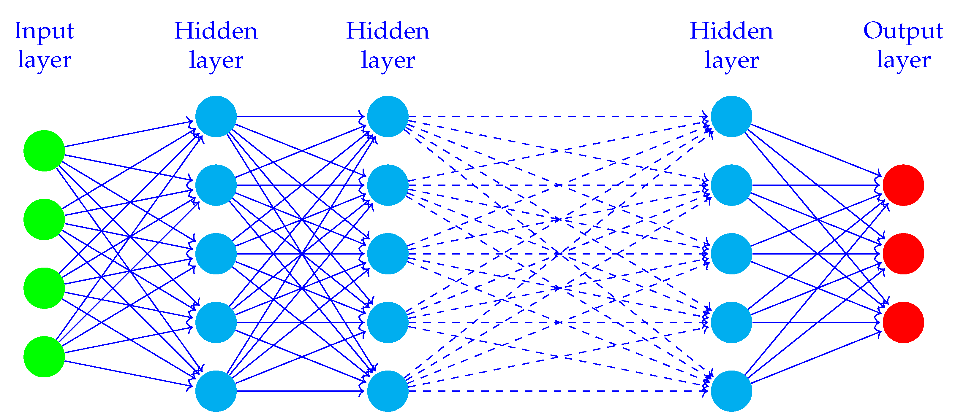
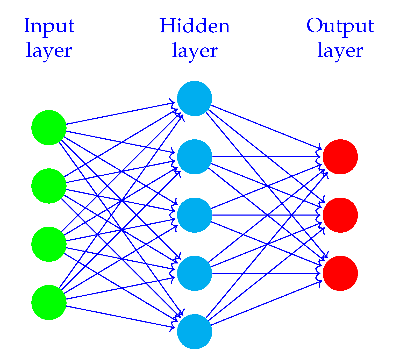
Artificial neural networks (ANN) emerged from considerations of perception and cognition in biology. Many of the ANN network architectures draw inspiration from the human brain. Figure 1 illustrates a simple ANN, where the circles illustrate nodes (neurons). Nodes belonging to the same layer are shown in one colour. Arrows illustrate weights, the connections between the layers. The figure shows that nodes belonging to the same layer are not connected, but nodes in consecutive layers are connected with weights. In the context of DL, “deep” refers to the number of layers contributing to a network. DL expands the ideas from simpler ANNs using deeper networks enabling them to capture more complex relationships between input and output variables.

Figure 2 illustrates a deeper version of the network displayed in Figure 1. A layer is a set of nodes. The connections between the layers are the trained units, also known as weights. The layers between the input and output layers are denoted hidden layers.

The values for each node are computed based on weights, biases and an activation function. For example to compute the node j in a layer l

$$a_j^{\left(l\right)}=g\left(\sum _{i=1}^n{w}_{i,j}^{\left(l\right)}{x}_i+b_j\right)$$

(1)

where $w_{i,j}^{\left(l\right)}$ represent the weighing of the inputs $x_i$ and $b_j$ the bias. The inputs $x_i$ can either be the input layer or the previous layer of the network, i.e., $x_i=a_i^{(l-1)}$. The function g represent the activation function, and must be set before the model training starts. Popular choices are rectified linear unit (ReLU), Sigmoid function ($\sigma$) or hyperbolic tangent (tanh), and their mathematical expressions are

$$ReLU\left(x\right)=\left\{\begin{array}{cc}\mathrm{x},\hfill & \mathrm{if}\mathrm{x}\ge 0\hfill \\ 0,\hfill & \mathrm{else}\hfill \end{array}\right.$$

(2)

$$\sigma \left(x\right)=\frac{1}{1+e^{-x}}$$

(3)

$$tanh\left(x\right)=\frac{e^x-e^{-x}}{e^x+e^{-x}}=\frac{e^{2x}-1}{e^{2x}+1}$$

(4)

The weights and biases of the network are trained (estimated) numerically by minimizing the loss (error) between the model outputs and the outputs in the training data using some pre-selected loss function.

2.2. Convolutional Neural Networks

Computer vision is a field of artificial intelligence concerned with interpreting the visual world. One popular model for visual tasks is the CNN.

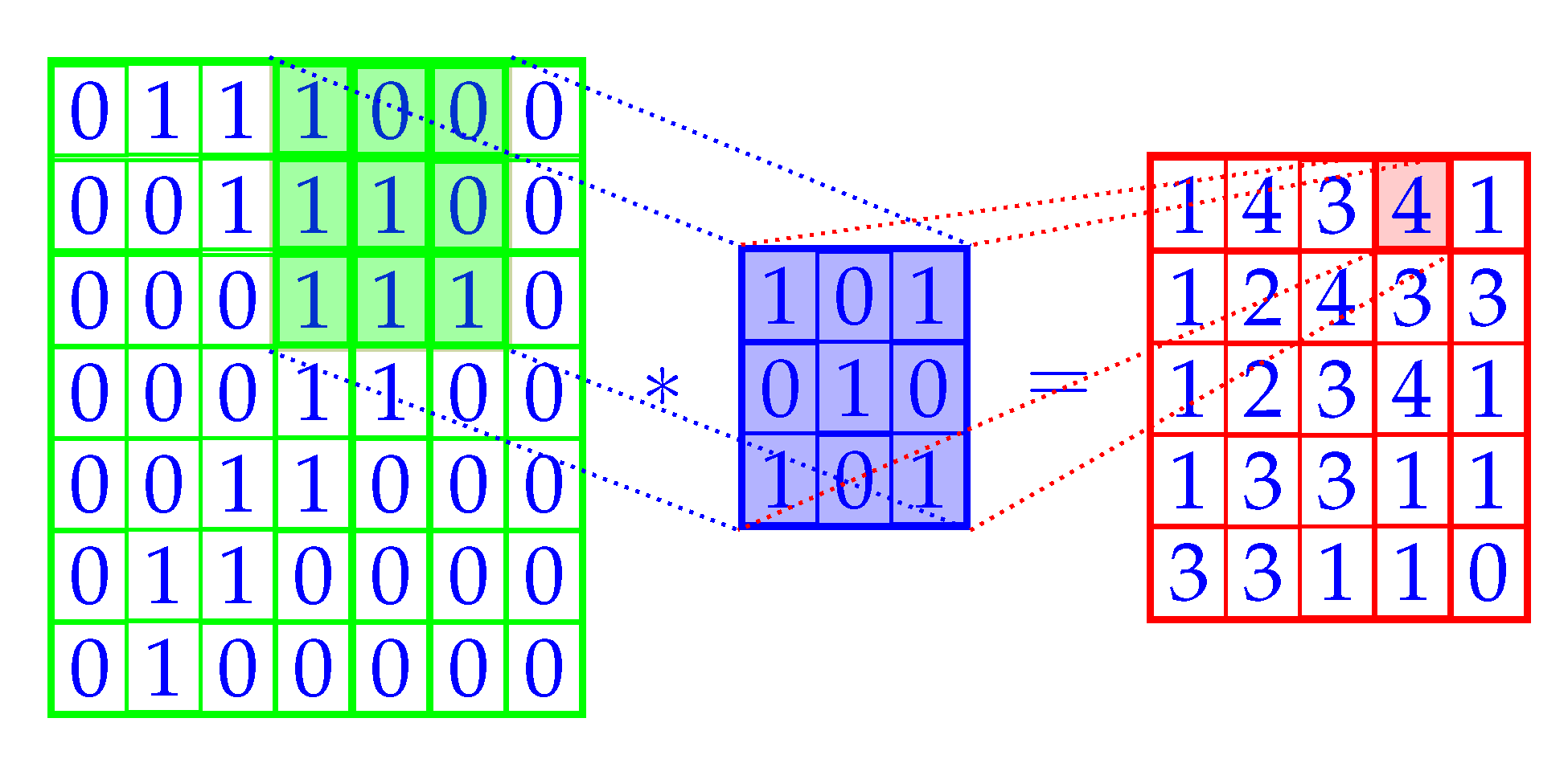
A core component of the CNN is the convolution mechanism. Several types of convolutions are used in CNNs, and Figure 3 shows one such convolutional operation as the sum over element-wise multiplication of the filter and input (shown with a *). The filter is blue, which is placed over the filled green section, producing the red output. The entire red grid is called a feature map (output map). The green grid is the input (typically an image), overlaid with blue indicating the pixels contributing to the activation, of the red pixel. In Figure 3 this would be the value 4. Receptive field is known as the pixels contributing to the activation in a pixel (i.e., the value) [20]. For instance, the receptive field of the shaded red pixel is the shaded green submatrix. Figure 3 shows the convolution of a single filter, but in practice the CNN model usually consists of many filters.

Unlike the fully connected neural network layers in the previous section, the nodes in the output layer are not connected to all the input nodes, but only the nodes within their receptive fields. One filter convolves the entire input, searching for a single characteristic of the input. When the filter finds this particular feature it activates, propagating this signal into the feature maps. A core idea of the CNN is to also train the values that should be used in the filters to optimize prediction performance, i.e., what kind of characteristics of the input should be emphasized for the given prediction task.

2.3. Padding

From Figure 3 we see that convolution operations shrink the dimensions of the feature map. We also see that the data along the border are less used than the rest of the data, and can reduce the accuracy of the DL predictions. A popular technique to avoid this is to use padding, which is based on putting zeros along the edges of the input. The degree of shrinking depends on the filter size $f\times f$, padding p and stride s. Stride determines how the algorithm convolve over the input. For some applications, including the one in this paper, it is useful to have the same shape of input and output. This is called “padding same”, and Equation (5) calculates the amount of padding necessary to preserve the dimension of the input volume.

$$p=\frac{n\left(s-1\right)-s+f}{2}$$

(5)

2.4. Recurrent Neural Networks

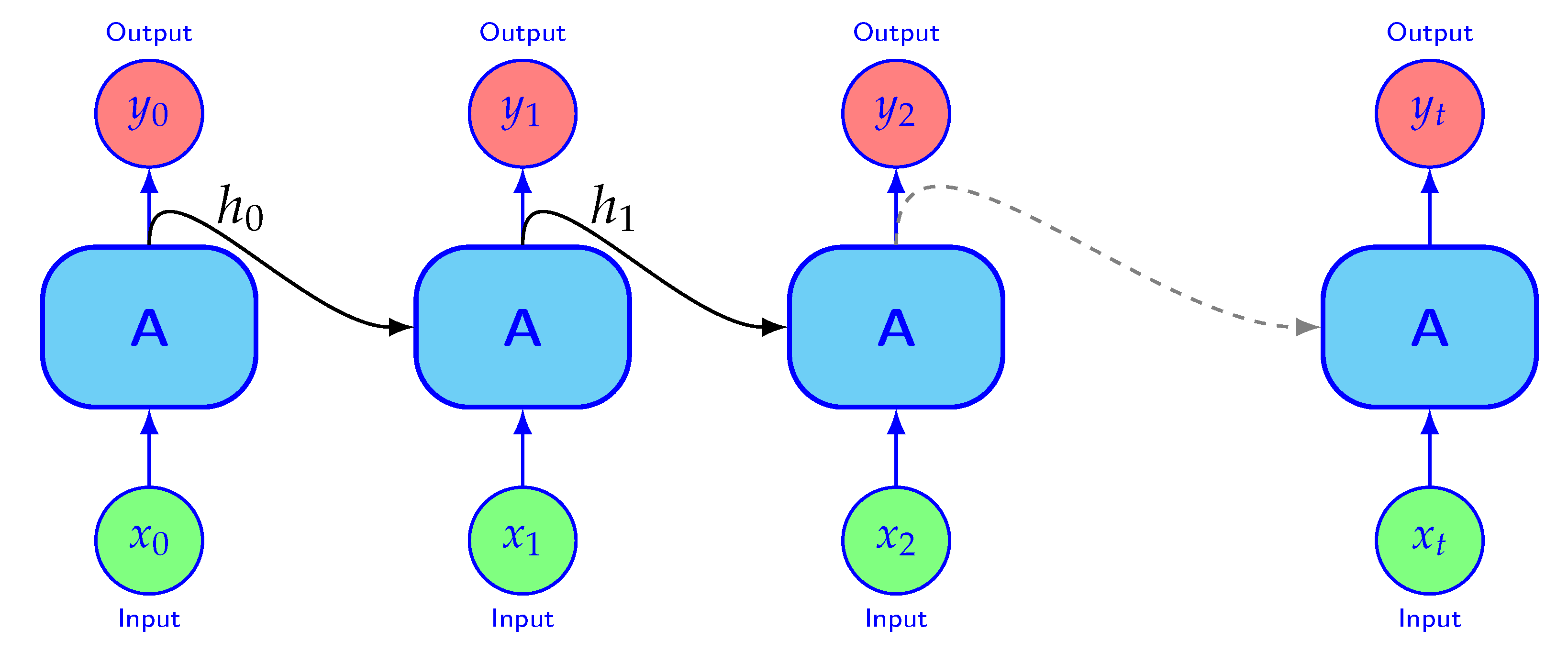
RNN is a class of ANNs developed for studying patterns in sequential data such as time series, audio or text. Figure 4 shows the structure of the RNN. The connection between the nodes are a directed graph along a temporal sequence. The hidden states $h_t$ from the previous step is fed into the next. The hidden states contain information about what has been learned so far. The “memory”, $h_t$, stores the useful information from the training sequence $x_0,x_1,\dots ,x_t$ that is useful to make efficient predictions of the output. For example, in weather forecasting, we can imagine that $h_t$ contains abstract information about the current state of the weather system that is useful to make precise weather forecasts.

2.5. Long Short-Term Memory Network

Unfortunately, training RNNs for long sequences turns out to be challenging. The optimization gradient can explode or vanish to zero. In order to address these challenges, Hochreiter and Schmidhuber suggested the LSTM Network [16]. The memory cells now contain input and output gates. A gate is a structure that can be opened or closed. Having values ranging from 0 to 1, it truncates the noise signal from the input and the output. Gers et al. 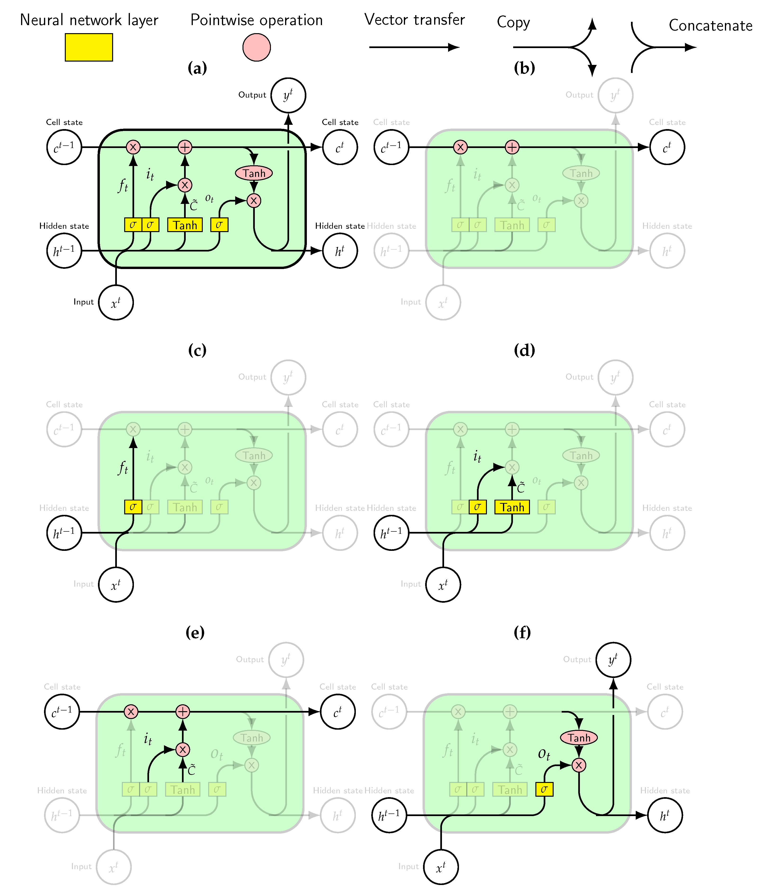[21] further suggested to add an additional gate, the forget gate. The idea was to enable the LSTM to reset parts of its own memory. Resetting releases internal resources and enables even more learning. In very simplified terms, the forget gate learns which part of the cell state, the long-term memory, it should forget. The input gate learns the information from the input it should add to the cell state. The output gate learns which information it should pass to the output. The assembled memory unit is displayed in Figure 5a. The information flow thought the cell is regulated by three gates; the forget gate (see Figure 5c), the input gate (see Figure 5d) and the output gate (see Figure 5f). These gates are all ANNs.

The long-term memory is shown in Figure 5b and the short term memory is referred to as the hidden state. The cell state is affected by some linear interactions, and usually simply results in an unchanged flow. The hidden state is the output passed to the next cell. Structures like gates regulate the flow of information.

To be able to make predictions the forward propagation of information through the network is required. Figure 5c shows this based on the new input and the previous hidden state, the forget gate determines which instances from the memory to remove. Regulating the information that stays in memory frees up space allowing the network to learn new things.

Figure 5d shows two processes, one determining the candidate information based on the input and another the computations in the input gate. The candidate information is filtered by the multiplicative input gate. This determines what information to add to the cell state.

Figure 5e shows how the cell state is updated. Using multiplicative gates, first the forget gate removes information. Then the output from the input gate adds the useful information from the input to memory. The input gate regulates what information to store from the input. The aim of the input gate is to clean the input by reducing the noise signal. These computations are also shown in Figure 5d.

Figure 5f illustrates how the output gate gets updated. Passing the cell state through the function tanh, it is given a value in the range from −1 to 1. The output gate determines what to remove from the cell state and pass as the hidden state. This gate aims to remove noise from the output, preventing misrepresentations of the hidden state (short-term memory).

A variant of the LSTM network is the ConvLSTM, which was originally developed for the application of precipitation nowcasting [22]. The difference between this and the general LSTM is that the standard ANNs of the LSTM (recall Figure 5a) are replaced by CNNs. This significantly reduces the number of variables in the model, making it possible to train LSTM models when the inputs $x_t$ and outputs $y_t$ are two dimensional, for example, images or observations in geographical grids.

3. European Cloud Cover Dataset

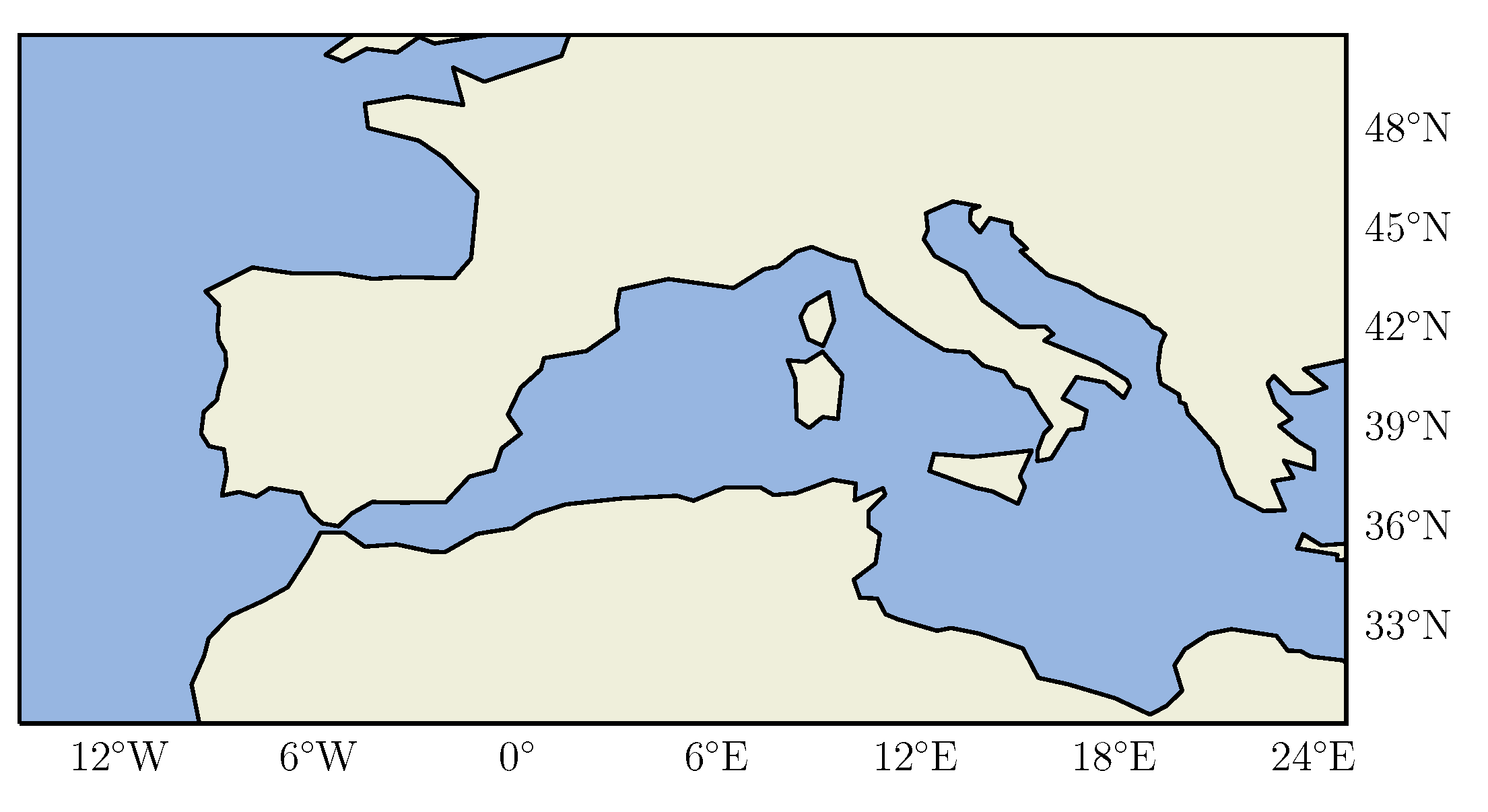
The ECC dataset consists of hourly data on a $0.{25}^{\circ }$ uniform grid resolution. The geographical domain is $[30,50]$ degrees latitude (north), and $[-15,25]$ degrees longitude (east), see Figure 6. The resulting dimensions of the grid are $81\times 161$ pixels. The domain covers Central Europe and North Africa. A total of $54\%$ of the domain is land, and $46\%$ is ocean or sea. The dataset was recorded from April 2004 to December 2018 and is comprised of the five variables; temperature (T), surface pressure (P), relative humidity ($RH$) and specific humidity ($SH$), and CFC. The ECC dataset can be downloaded from https://datasets.simula.no/ecc-dataset/, accessed on 1 November 2021.

The ECC dataset is compiled by two sources of data. T, P, $RH$ and $SH$ were collected from the 5th Generation Reanalysis data (ERA5) from the European Centre for Medium-Range Weather Forecasts [23]. Reanalysis is as close to observations as one can get while still obtaining complete and coherent data in both space and time. It is produced using a forecast model to assimilate observations. Data assimilation takes observations as input and tries to make an accurate estimate of the state of the system that is as consistent as possible with the available observations at all times. This includes observations retrieved from satellites, ships, buoys, airplanes, and ground-based stations. There are multiple global reanalysis datasets available, and they are all different. It depends on the forecast assimilation system used and observations assimilated [24]. ERA5 was used because of its fine resolution and recent release date of January 2020.

The variables were all retrieved from the surface (T, P) or the closest pressure level (1000 hPa) ($RH$ and $SH$). We wanted to investigate to what extent surface observations can be used to predict clouds. The reanalysis data also offers information about humidity at other pressure levels but is more modelled than real observations. Many prevalent types of clouds form by air parcels close to the surface being heated from below, becoming buoyant and ascending through the atmospheric columns while simultaneously cooling, often to the point where water starts to condense and a cloud is formed. For these cloud types, temperature and humidity near the surface are key variables. Other cloud types, for example those associated with weather fronts, are less tightly linked to near-surface variables, but the passage of a weather front brings in air masses of different temperature and humidity both at the surface and aloft, and thus near-surface variable may still be good indicators of frontal clouds even though they do not have a direct influence on the cloud formation.

The second source is METeosat Second Generation (MSG) cloud masks from the European Organisation for the Exploitation of Meteorological Satellites (EUMETSAT) [25] and was selected due to its high spatiotemporal consistency and resolution. The variable cloud masks are provided by many satellites, bringing valuable information in itself, but also for the retrieval of other variables restricted to cloud free conditions [26]. The cloud masks were further regridded to the same grid as the ERA5 data [12]. MSG has used the four different satellites for the data collections from the start in 2002, namely the METeosat-8 to METeosat-11, covering different time periods. To create the ECC dataset, data from all four satellites were used.

4. Cloud Fractional Cover Prediction Models

A potential alternative to use NMCs for projecting future CFC is to use a statistical downscaling procedure (by future CFC here we mean future from a climate perspective, i.e., for example the time period 2030–2100). For further descriptions about statistical downscaling see e.g., [8].

• Train a model to predict CFC from T, P, $RH$ and $SH$ using the ECC data, $CF{C}_H=f(T_H,P_H,R{H}_H,S{H}_H)$. The subscript H is added to emphasize that the relation is trained based on historic observations.
• Let $T_F$, $P_F$, $R{H}_F$ and $S{H}_F$ denote projections of future values of these variables from NCMs, for example for the time period 2030–2100. Project future values of CFC using the trained model from step 1, i.e., $CF{C}_F=f(T_F,P_F,R{H}_F,S{H}_F)$

The environmental variables T, P, $RH$ and $SH$ were selected for two reasons. First, the variables are predicted well in NCMs which is a requirement for the second step of the procedure to be reliable. Second, we expect that it should be possible to predict CFC from these variables. For example, high humidity is usually a requirement for cloud formation.

As pointed out in Section 1, we focus on the first step of the statistical downscaling procedure above, i.e., we will focus on evaluating the ability of the ConvLSTM model and the regression equation to predict CFC from the environmental variables on historic data. We will not do the second step of the procedure but is still added to motivate for why we do the model training and evaluations we do in this paper.

4.1. Convolutional LSTM Architecture

We suggest a ConvLSTM-based model due to its ability to learn complex spatial and temporal patterns. The model takes a 24 h sequence of values of T, P, $RH$ and $SH$ as input to predict CFC for the same 24 h sequence in accordance with the first step of the procedure above. Each sequence started at 00Z. We used such a long sequence to give the model the ability to learn the complex spatiotemporal patterns in cloud formation. 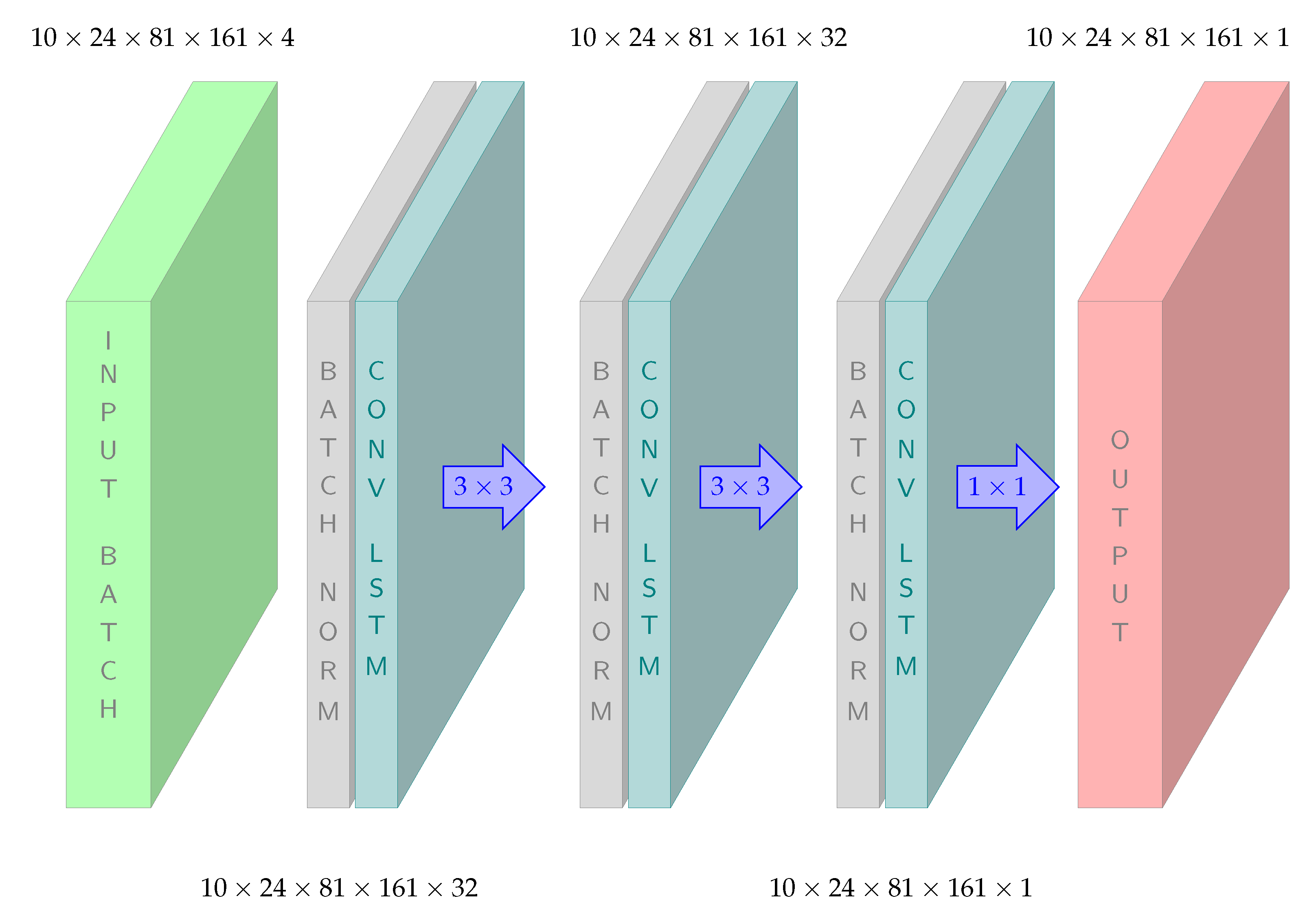Figure 7 shows an example of a model architecture we explored.

For the input batch the numbers 10, 24, 81, 161 and 4 refer to the number of batches, sequence length (hours), geographic dimensions and number of variables (T, P, $RH$ and $SH$), respectively. The model is further followed by batch normalization [27] and ConvLSTM layers. We see that in total three such architectures were used between input and output, where the output from the previous batch normalization are inserted to the next ConvLSTM, then further from ConvLSTM to batch normalization and so on. Batch normalization refers to standardizing the outputs from the previous layer of the network such that the mean value and standard deviations of the outputs from the previous layer are zero and one before computing the next layer of the network. The values 32 and 1 refer to the number of hidden states (recall Figure 1) and the $3\times 3$ and $1\times 1$ arrows refer to the sizes of the convolutional filters in the ConvLSTM layers (recall Figure 3). The results showed three benefits, the network was less sensitive to initial values for the weights in the optimization (training) algorithm, higher learning rate (how fast the algorithm learns from the training data) and dropout was not needed. Dropout is a technique often used in DL to avoid overfitting, and based on randomly setting the values of some weights equal to zero. Disabling dropout accelerated the training process. “Padding same” (Section 2.3) is applied to all ConvLSTM layers to make sure the input and output dimensions were the same. This is a natural requirement since the dimensions of the input (the environmental variables) and the output (CFC) is on the same grid. For the experiments in this paper we decided on five different configurations of the ConvLSTM based on empirical testing of the different possible configurations of hidden states and filter sizes, etc.

4.2. Multiple Regression Equation

As mentioned before, we also evaluate the performance of a multiple linear regression equation. Linear regression equations are the most common to use in the two-step statistical downscaling procedure [28]. In each geographical location, we fitted the regression equation

$$CFC={\alpha }_0+{\alpha }_{1}T+{\alpha }_{2}P+{\alpha }_{3}RH+{\alpha }_{4}SH$$

(6)

to predict CFC at a given time point from the values of T, P, $RH$ and $SH$ at the same time point in accordance with the first step of the statistical downscaling procedure described above. Here ${\alpha }_0$ is the regression intercept with the y-axis and ${\alpha }_1-{\alpha }_4$ the regression equation constants for each variable.

5. Computer Experiments

The ECC dataset was divided in training (2004–2012), validation (2012–2013) and test (2014–2018) sets. The overall aim is to predict CFC from T, P, $RH$ and $SH$ for the test period. The experiments were run on a DGX-2 system consisting of 16 NVIDIA Tesla V100 GPUs, each of 32 Gb local memory and 1.5 Tb of shared memory.

The ConvLSTM was implemented using Tensorflow’s Keras API [29]. The weights of the ConvLSTM were initialized based on the scheme “LeCun uniform” [30], and optimized with the Adam optimizer using the standard settings, $\mathrm{learning}\mathrm{rate}=0.001$ (tuning parameter for step size per iteration), ${\beta }_1=0.9$, ${\beta }_2=0.999$ (decay rates used for estimating the first and second moments of the gradient) and $ϵ={10}^{-7}$ (constant for numerical stability) as defined in [31]. Usually, in Tensorflow the $ϵ$ is set to ${10}^{-8}$ which we changed to ${10}^{-7}$. This was done to avoid the optimizer becoming unstable, which can happen with a smaller $ϵ$. The loss function was mean squared error. The training procedure reached convergence both in terms of training and validation loss. The models predicted almost equally well on the unseen test data compared to on the training set, indicating the models did not suffer from overfitting. The prediction error was measured using mean absolute error (MAE).

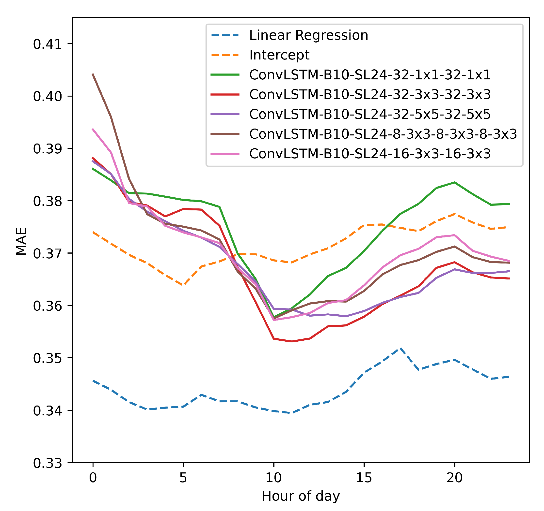
Figure 8 shows the prediction performance for the different models for different hours of the day. The error is also averaged over all the geographic locations. Uncertainty bounds are not added to the plotted curves since given the large number of test examples, the uncertainties in the plotted curves are minimal.

Intercept refers to a model that predicts without using the features, i.e., the prediction is based on the average CFC in the training data. This is equivalent to fitting a regression equation only consisting of the intercept ${\alpha }_0$. The regression equation outperformed the ConvLSTM, but also the best ConvLSTM models performed better than the intercept for most hours of the day documenting that the ConvLSTM was able to learn from the features. Cloud formations are often more active in the afternoon due to surface heating increasing as the sun rises, and might explain the increased prediction error for the regression equation and the ConvLSTM in the afternoon. Further, we see that neither the ConvLSTM nor the regression equation improve much on the intercept documenting that predicting CFC is a difficult problem.

Table 1. Mean absolute error (MSE) for different regression equations taking the average over all geographic locations and time points. The second column refers to MSE for regression equations only using T as a feature. The third to the fifth columns are the same, but with only P, $RH$ and $SH$ as the feature, respectively. The sixth column shows the MSE using all the four environmental variables as given in Equation (6) and the seventh column is a regression equation without any of the environmental variables, i.e., only the intercept.

Reg. Equation	T	P	RH	SH	All	Intercept
MSE	0.357	0.363	0.367	0.360	0.344	0.372

shows the MSE when predicting CFC for different regression equations. The MSE is computed taking the average MSE over all geographic locations and time points in the test set.

We see that all the regression equations consisting of a single feature perform poorer than the full model and better than the intercept, indicating that each environmental variable to some extent contributes to the prediction in the full model. Among the features temperature is the one being most efficient in predicting CFC.

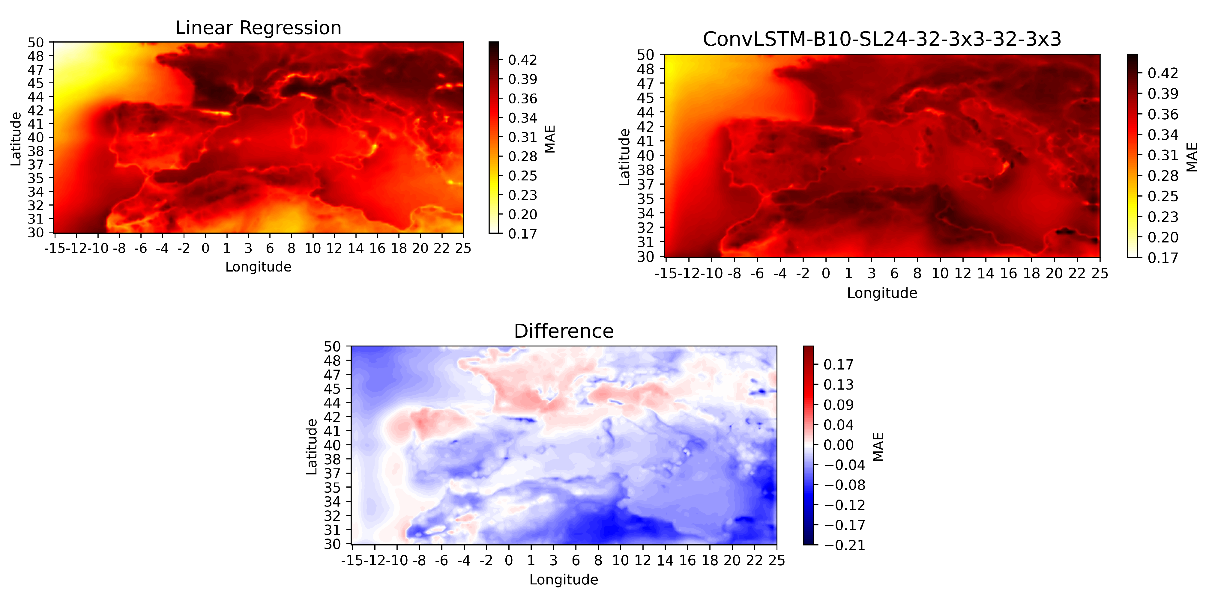
Figure 9 shows prediction error in different geographic locations.

We see that for most of the geographic area, the regression equation performs the best. However, especially along the coast of Spain, France and the Northern Mediterranean Sea and in the Alps, the ConvLSTM performs best. This might indicate that the ConvLSTM models are better at predicting CFC for areas with land/sea interactions or areas where convergence may initiate convections, e.g., along mountain ridgelines leading to phenomena such as orographic lifting.

6. Conclusions

In this paper, we have evaluated the potential of using the ConvLSTM model and a regression equation to predict CFC from other environmental variables. A potential application of the models is, as part of the two step statistical downscaling procedure, described in Section 4. The selected environmental variables were chosen since they (i) are modelled well in NCMs and (ii) and could potentially contain information to predict CFC, both being necessary requirements for the statistically downscaling procedure to be meaningful. To the best of our knowledge this is the first attempt in this direction.

The results showed that the ConvLSTM models were outperformed by the linear regression equation, showing that the ConvLSTMs were not able to predict CFC on the level we had expected. Neither the ConvLSTM nor the regression equation performed much better than the intercept indicating that it might not be much information in the environmental variables to predict CFC. A potential direction for future research could be to look for other input information that could potentially improve the predictions of CFC and in the end the projections of future CFC using statistical downscaling.