Article

TranScreen: Transfer Learning on Graph-Based Anti-Cancer Virtual Screening Model

by
Milad Salem
1,†,
Aminollah Khormali
1,†,
Arash Keshavarzi Arshadi
2,
Julia Webb
2 and
Jiann-Shiun Yuan
1,*
1
Department of Electrical and Computer Engineering, University of Central Florida, Orlando, FL 32816, USA
2
Burnett School of Biomedical Sciences, University of Central Florida, Orlando, FL 32816, USA
*
Author to whom correspondence should be addressed.
Equal Contributions.
Big Data Cogn. Comput. 2020, 4(3), 16; https://doi.org/10.3390/bdcc4030016
Submission received: 19 May 2020 / Revised: 17 June 2020 / Accepted: 23 June 2020 / Published: 29 June 2020

Abstract

:
Deep learning’s automatic feature extraction has proven its superior performance over traditional fingerprint-based features in the implementation of virtual screening models. However, these models face multiple challenges in the field of early drug discovery, such as over-training and generalization to unseen data, due to the inherently unbalanced and small datasets. In this work, the TranScreen pipeline is proposed, which utilizes transfer learning and a collection of weight initializations to overcome these challenges. An amount of 182 graph convolutional neural networks are trained on molecular source datasets and the learned knowledge is transferred to the target task for fine-tuning. The target task of p53-based bioactivity prediction, an important factor for anti-cancer discovery, is chosen to showcase the capability of the pipeline. Having trained a collection of source models, three different approaches are implemented to compare and rank them for a given task before fine-tuning. The results show improvement in performance of the model in multiple cases, with the best model increasing the area under receiver operating curve ROC-AUC from 0.75 to 0.91 and the recall from 0.25 to 1. This improvement is vital for practical virtual screening via lowering the false negatives and demonstrates the potential of transfer learning. The code and pre-trained models are made accessible online.

1. Introduction

Drug development is a long and costly process during which a drug candidate is discovered and widely tested to be both efficient and safe. This process can take an average of 12 years with billions of dollars spent per drug [1,2]. The early stages of this process involve discovery of a drug candidate which is bio-active towards the targeted disease and is non-toxic for humans. Since High Throughput Screening (HTS) of big library of molecules for discovery of a potent scaffold is very inefficient, for decades, scientists have been working on modeling the bio-activity in silico and virtually screening the molecules. Since the screening takes place in simulation with no wet-lab effort, the cost and time of early drug discovery can be drastically decreased.
Traditionally, molecular descriptors and fingerprints are used to extract features from the input molecules, which are then passed to a machine learning model for training. This pipeline has been used for many virtual screening tasks such as kinase inhibition prediction [3], side-effect prediction [4], cytotoxicity prediction [5], and anti-cancer agent prediction [6]. In the recent years, deep learning models have proven to be capable, and in some cases superior [7], virtual screening tools for predicting the bio-activity of given molecules. The automatic feature extraction offered by deep learning models has been demonstrated to enable de novo drug design [8], Pharmacokinetics profile prediction [9], and bio-activity prediction [10]. Since the performance and accuracy of the screening models have a direct effect on the outcome of drug development pipelines [11], deep learning offers practical virtual screening. However, deep learning models are over-parameterized and data hungry models, thus face challenges in the virtual screening domain. These challenges are at heart of what this work examines and aims to address.
One of the main challenges of virtual screening is over-fitting on the imbalanced and small training datasets [12]. In most molecular training datasets, the active molecules are rare and make up the minority distribution in the dataset, with inactive molecules outnumbering them heavily. Moreover, the number of total data points within available datasets is low due to the cost of screening in vitro. The significance of this challenge becomes palpable when a virtual screening model is trained on a non-diverse training dataset and tested on a large and diverse dataset. This scenario is often the case in many virtual screenings for drug discovery [13], and needs to be addressed for models to be practical in real-world applications.
A handful of solutions have been adapted to virtual screening from other domains of deep learning to battle this challenge. For virtual screening drug discovery, the problem of low and imbalanced data is handled traditionally using expert-made features [14], and in more recent years with a few applying multitask learning [15], few-shot learning [16], and unsupervised pre-training [17], with results showing performance improvement or deterioration in various cases. Transfer learning, which is the focus of this work, allows better initialization of the models and alleviates the problems caused from over-parameterization and imbalanced datasets. A wide-scale study of transfer learning, a collection of models to transfer from, and the study of models’ behavior are lacking from the virtual screening domain.
The main aim of this work is to apply transfer learning for a virtual drug screening in a wide-scale manner. A p53-based dataset is chosen as the virtual screening task due to its importance for anticancer discovery, the imbalanced property of the dataset, and the fact that high sensitivity to weight initialization is observed in its baseline model. The results are compared to a related work, which uses reinforced multi-task learning to classify the same task [18]. The behaviors of the models are analyzed via ranking the model’s predicting capability before its training on target data. The main contributions of this work are:
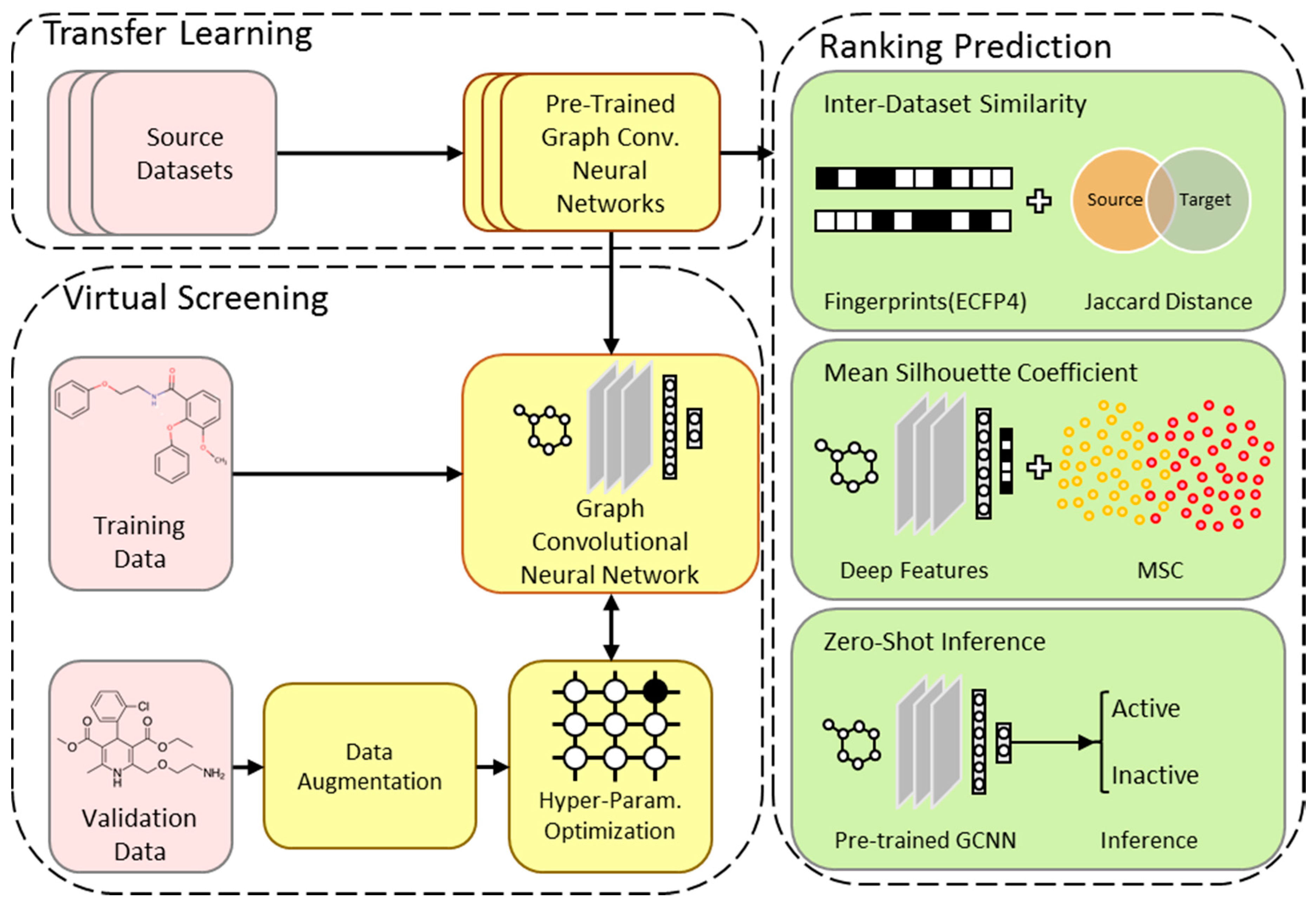
  • TranScreen pipeline: A practical pipeline is developed, which enables the usage of graph convolutional neural networks (GCNNs) for virtual screening and transferring the learned knowledge between multiple molecular datasets.
  • Creation of a collection of weights, which can be used as network initializations.
  • Comparing three methods of ranking models before fine-tuning takes place to select the model for future tasks.

2. Materials and Methods

2.1. Overview of the TranScreen Pipeline

The pipeline implemented in this work aims to apply transfer learning to a graph-based virtual screening model in a practical manner. The source datasets (from MoleculeNet) used for transfer learning and the target dataset (related to cancer) offer simple molecular-input line-entry system (SMILES) strings as input, and bio-activity or inhibition class as output to the models. The datasets are preprocessed and partitioned based on scaffold into training, validation, and test splits. As seen in Figure 1, one common network architecture and set of hyper-parameters are chosen. The source datasets are used to train multiple GCNN models with the common architecture in their related task. The pre-trained networks are then transferred to the target task and the models are fine-tuned. The models are ranked based on how well they perform on the target test dataset. Three different approaches are implemented which use the source data, the deep features of the target validation dataset, or zero-shot inference to predict the rank of the pre-trained models before fine-tuning.

2.2. Data

2.2.1. Source Data

MoleculeNet [19] is a large-scale molecular database designed to enable machine learning model creation for molecular tasks. This database offers a unique collection of multiple tasks and diverse molecules, which makes it an ideal choice for transfer learning. The source datasets used in the TranScreen pipeline are chosen from MoleculeNet datasets that have SMILES information. These source datasets originate from six different datasets, namely PCBA, MUV, HIV, BACE, Tox21, and SIDER, consisting of in total 182 tasks (assays) and 582,914 molecules. The datasets are not combined, yet each task is taken as an independent dataset, creating 182 different source datasets which can be used to train the same number of source models. We have provided detailed statistics for each dataset in Table 1. Detailed information about name of the tasks is provided in the Appendix B.

2.2.2. Target Data

The p53 gene is mutated in roughly 50–60% of all human cancers [20], making it an important target for the understanding and treatment of cell abnormality. As it is mentioned in Appendix A, it is not entirely clear what pathways would become involved after p53 mutation and loss of function. Therefore, not all molecular targets of the resultant cancers are known, and prediction of candidate drugs is not always feasible. Therefore, we identify four p53-based datasets (PCBA-aid902/aid903/aid904/aid924) in which high throughput screening assays were performed to discover potential anticancer compounds. Since the molecules need to be potent against a cell line with no p53 expression (complete loss of function), which is still mutated and cancerous, PCBA-aid904 [21] is chosen as the target dataset, which used a p53 null cell in a non-permissive temperature assay. By doing so, scaffolds selectively inhibiting cancer cells with loss of p53 functionality can be predicted. Since the target data is from PCBA dataset of the MoleculeNet, it is removed from the source data. The three other tasks, namely PCBA-902, PCBA-903, and PCBA-924, were also deleted due to the close relation they had with the target dataset. The information regarding the target dataset is presented in Table 2. Due to the low number of active compounds, this dataset is highly imbalanced and only 0.12% of the molecules show bio-activity.

2.2.3. Data Preprocessing and Partitioning

During preprocessing, SMILES with bio-activity data are read from each dataset. The input SMILES do not need to be canonical since the model will rearrange the input atoms in a preset order. Chirality information can be included in each input in order to distinguish between isomers. For each task, 80% of the compounds are selected as training samples, while the rest are partitioned as test and validation dataset. Dataset partitioning is done in regards to scaffolds of the molecules, which ensures that similar molecules are put in same data splits and increases the variation between training, test, and validation splits.
The validation set is aimed to be used to tune the process and to find the optimum model. If this validation set is chosen at random from a non-diverse dataset, the model may be prone to memorization of specific features that represent the homogenous training distribution. The random partitioning will decrease the trained model’s ability to be applied to unseen test datasets. Therefore, dataset partitioning is implemented based on scaffolds of the molecules to improve generalization abilities of the learned representations and increase the practicality of the model in real-world scenarios.

2.3. Model Creation and Training

2.3.1. Graph Convolutional Neural Networks

Traditionally, virtual screening models take fingerprints of the molecules as input representation [14]. One of the most popular fingerprint creation techniques is Extended Connectivity Fingerprint [22], which encodes the existence of specific sub-structures of the molecule into a binary array. In recent years, this technique has been improved with the addition of GCNN models [10]. These deep learning models learn from the data to extract useful feature representations during training, while building on the same concepts of circular fingerprints.
GCNNs have been successfully applied to many tasks in drug discovery such as drug-target interaction prediction [23], physiochemical properties prediction [15], and chemical reaction prediction [24]. Part of this success is owed to the fact that molecules inherently resemble graphs, with nodes representing atoms and edges representing the bonds between the atoms. In this work, the DeepChem [25] implementation of GCNNs with Tensorflow backend are used. This framework also handles the conversion of molecules to graphs with featurization of atom types, atom bonds, number of Hydrogens, and formal charge.

2.3.2. Common Network Architecture

One common model architecture and set of parameters need to be defined so that all models within the pipeline can be transferred to the target task. An architecture that has proven to perform well on the molecular dataset or task can be chosen as the common architecture. Alternatively, hyper-parameter optimization can be done using a grid search over various parameters and using the validation data to find a best-performing model. However, in many cases in virtual screening, the validation data is highly imbalanced and the effects of active molecules on the result of the grid search are diminished. Therefore, we suggest using data augmentation in the form of SMILES Enumeration [26], in order to make more copies of the active molecules and make the validation set balanced. Thus, more importance is put on finding active molecules when searching for optimum hyper-parameters. In this work we use an architecture that has proven to perform well on the PCBA dataset as the common architecture. This architecture is adapted from our previous work [27] which implements the aforementioned data augmentation and hyper-parameter optimization. The details of the common architecture are given in Table A1.

2.3.3. Baseline Model and Internal Validation

After the data is preprocessed and the model is defined, training on the target task can begin. The training set from the target data is used to train the GCNN with random initialization for 30 epochs. Over-training was avoided using internal validation; the model is saved at each epoch during training and the performances of the model on the training set and the validation set are compared. In a healthy training period, the model’s performance is improved over time on both sets. However, when over-training occurs, a decline in performance is observed on the validation set. The model from the last epoch before over-training, which is the second epoch, is taken as the base-line model.

2.4. Transfer Learning and Fine-Tuning

Machine learning has been successfully applied to many fields such as natural language processing [28], speech recognition [29], structured data [30], and arguably most predominantly to the image domain [31]. The current state of the solutions to low and imbalanced data in the image domain include the use of data augmentation [32], multitask learning [33], few-shot learning [32], and general transfer learning [34]. The training procedure of the deep learning models can be highly sensitive towards the weight initialization. Authors in [35] demonstrated that in most initializations there is a winning set of weights that become dominant during training. The stochastic gradient descent procedure will focus on this sub-structure of the network, making the rest of the network susceptible to be removed during pruning. This sheds a new light on how network initialization affects the training and performance of a deep learning model. Unfortunately, the situation is exacerbated when deep learning models are used as virtual screening models, since they are over-parameterized models that are data-hungry and are faced with imbalanced, non-diverse, or small datasets.
The state-of-the-art solution in dealing with the initialization challenge would be the use of transfer learning [34]. This process can include the transfer of weights from a pre-trained model on one domain (source) to a model on another domain (target). These weights represent what the source model has learned from the source data and the patterns used to extract features from the data. Transfer learning has shown to improve performance in many cases, but also hurt the performance in some [36]. Transfer learning in virtual screening has also been sparsely implemented in the forms of multitask learning [15] and unsupervised pre-training [17].
In this work, a separate GCNN model is trained for each source task, making a total of 182 source models. These tasks are of different data size, data diversity, and biological origin. Each model is trained for 30 epochs and the weights are saved and transferred to the target task. The models are then fine-tuned on the target training set for one epoch.

2.5. Model Rank Prediction Before Fine-Tuning

After the models are trained, fine-tuned, and evaluated they can be ranked based on how well they performed on the target test dataset. An interesting question arises: can this ranking be predicted before fine-tuning on the target dataset was initiated? If there can be a rank prediction method, useful recommendations can be made for future tasks and there would not be a need to apply large scale transfer learning from all 182 models. This question is a derivative of domain shift [37] and requires the comparison of the nature of datasets and models from the source and target domains. There are two main approaches in the literature for ranking pre-trained models, either via training an alternative model [38,39] or via statistical methods [36,40,41]. In this work we implement two of the statistical methods and offer a third solution in order to take a step forward in model rank prediction.

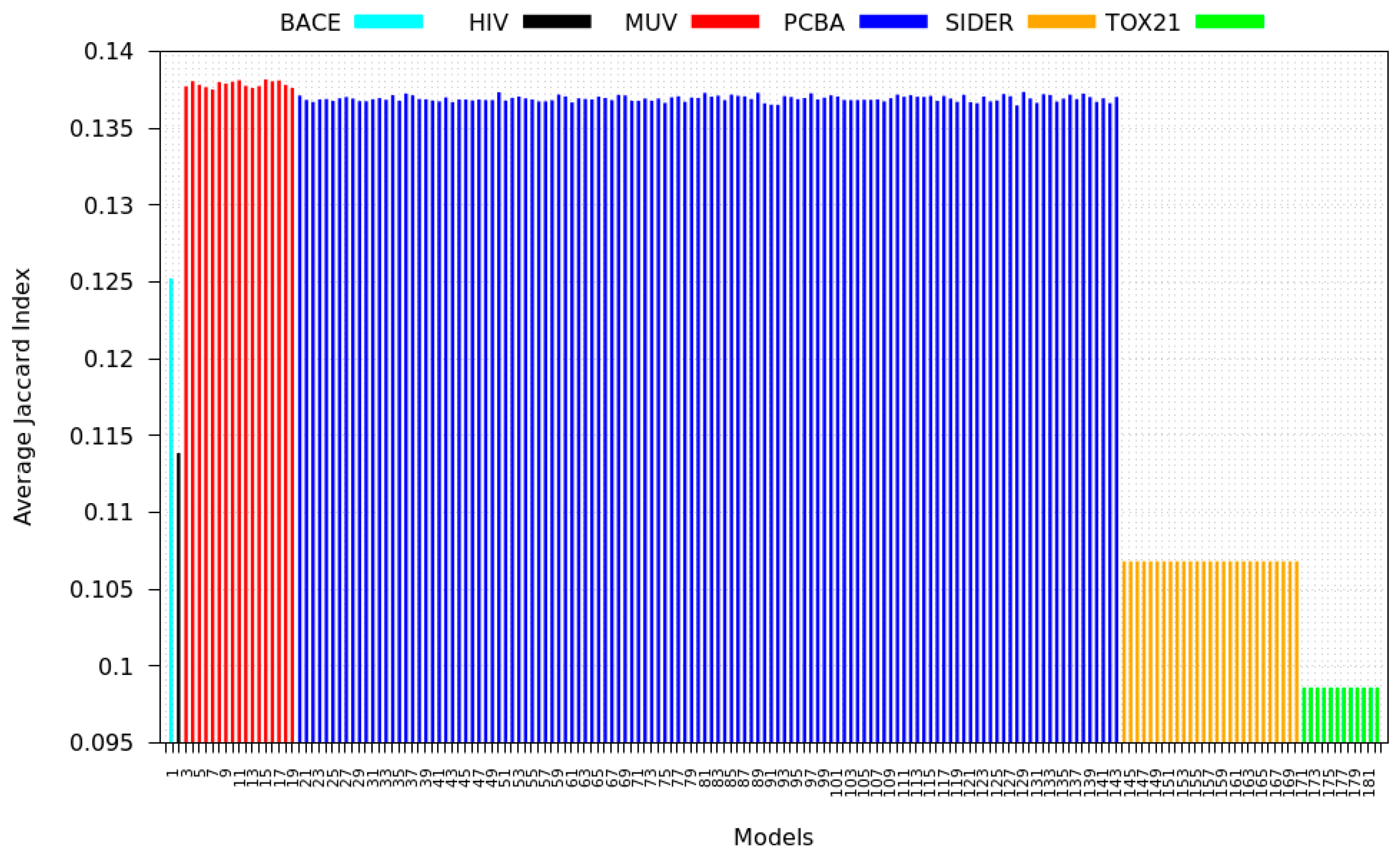
2.5.1. Inter-Dataset Similarity Comparison

The intuitive solution for model ranking prediction is to examine the source and target datasets and find the similarity between them [42]. If the model has seen similar data during training on the source dataset, it might have learned useful representations for the target task. This intuition can also be seen in traditional virtual screening models, which are based on the concept that molecules that share common sub-structures (i.e., fingerprints) and have similar bio-activity. In this work, this method is adopted from time-series domain in the form of Inter-Dataset Similarity (IDS) comparison [36] and is implemented using ECFP molecular fingerprints. The Jaccard (Tanimoto) Coefficient is used to find the pair-wise similarity between molecules from the source dataset and the molecules from the target dataset. The results are averaged over the maximum of 10,000 molecules, due to the large size of calculations. Higher Jaccard Index represents more similarity between the datasets.

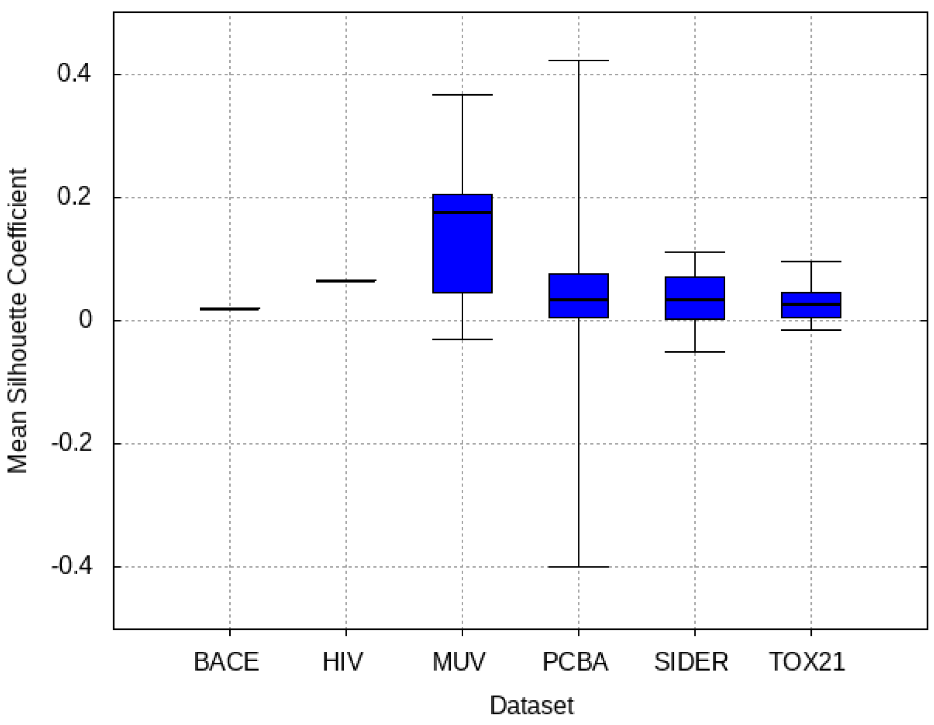
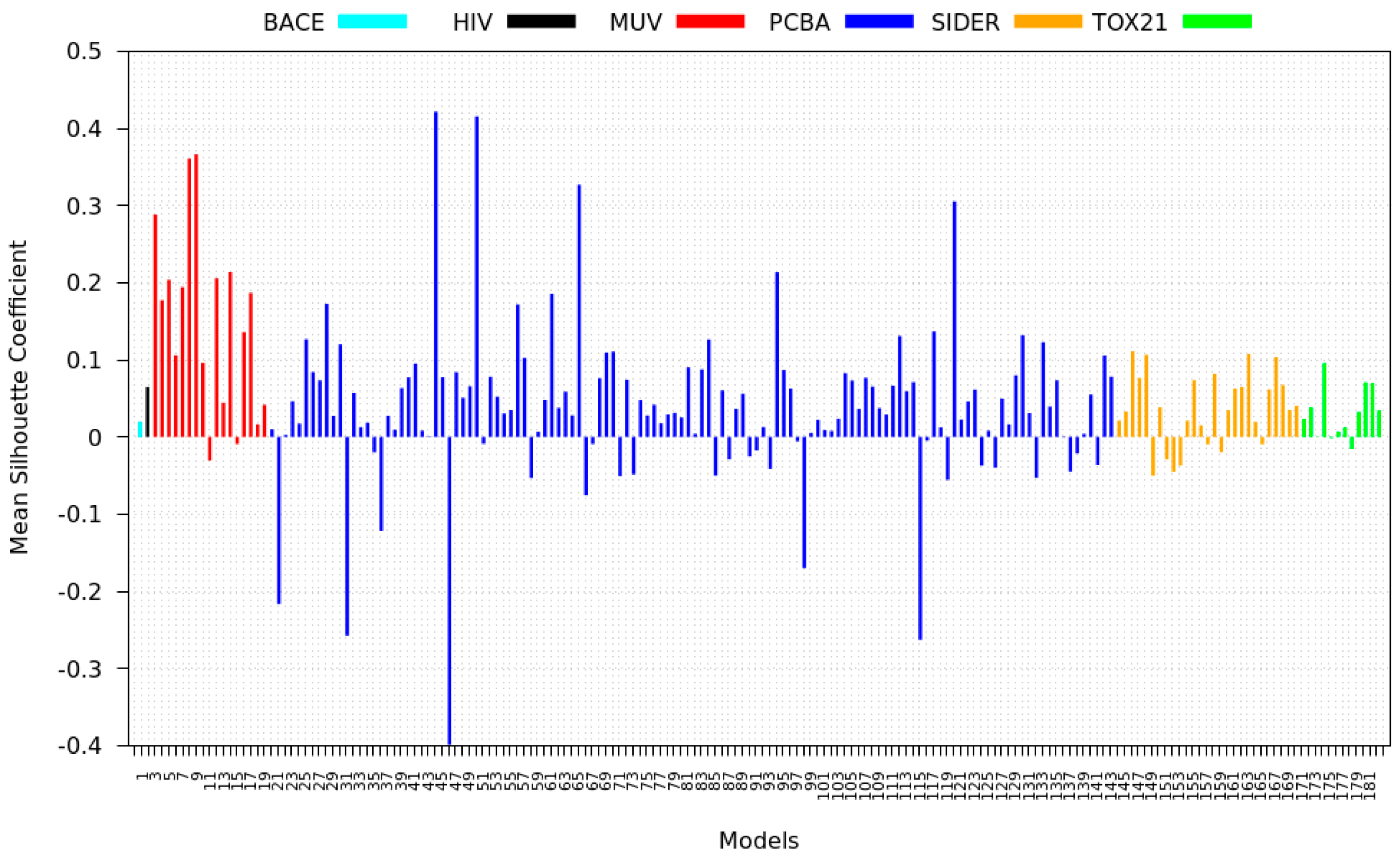
2.5.2. Mean Silhouette Coefficient on Deep Features

The second solution for ranking prediction is to understand how well the models distinguish between active or inactive target molecules. If the model’s inner representations are able to discriminate based on the activity of target molecules, it might be easier to fine-tune the model and thus perform better on the target task. In order to do so, the Mean Silhouette Coefficient (MSC) calculation is adopted from the time-series domain [41] as the ranking prediction metric. This metric is used to evaluate the efficiency of a clustering algorithm based on how distinguished the clusters are from each other. This metric is applied to features extracted from the second to last layer of the model, in order to judge how well these features distinguish between active and inactive molecules from the target validation dataset. Higher MSC represents better discrimination between the clusters.

2.5.3. Zero-Shot Inference
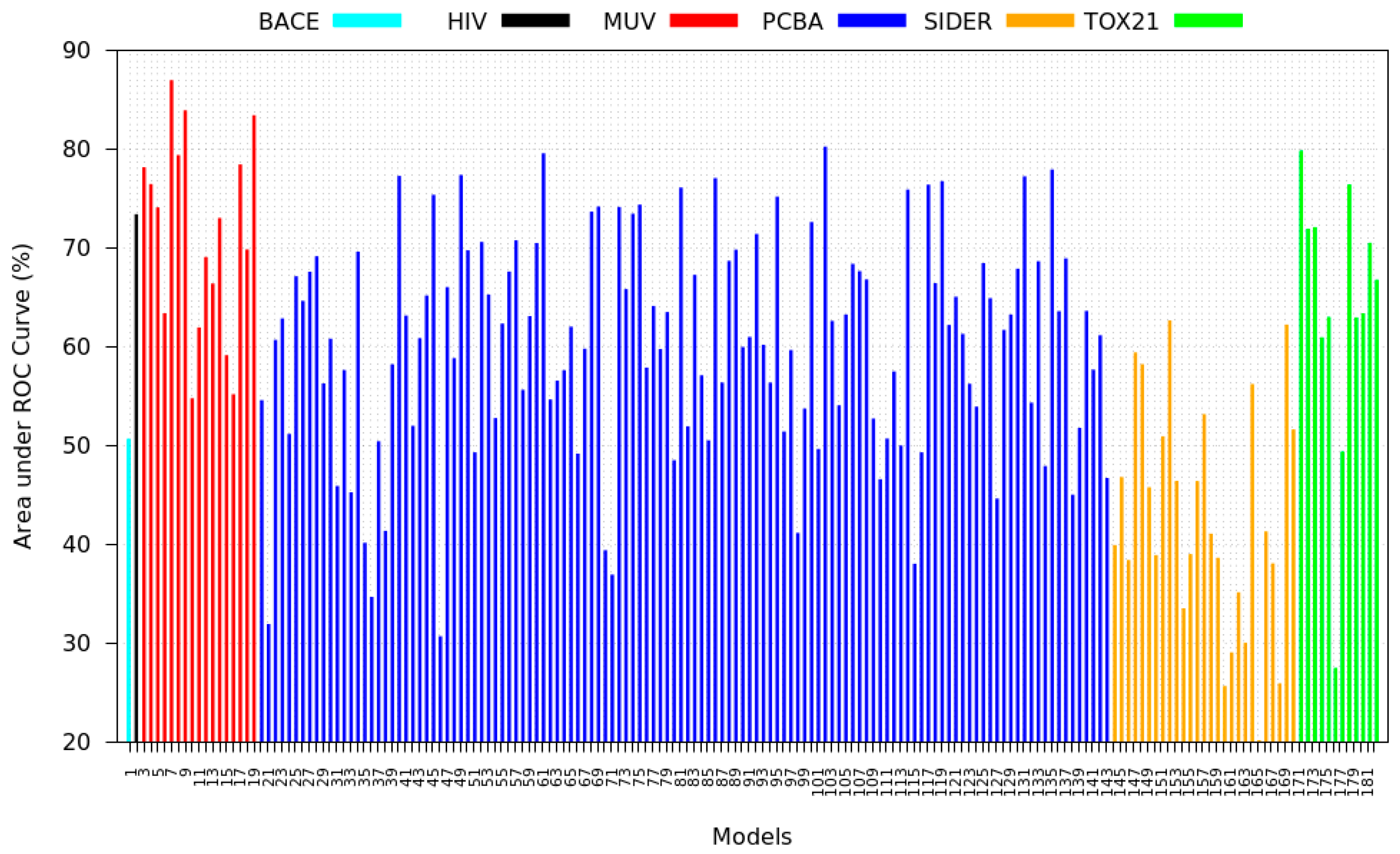
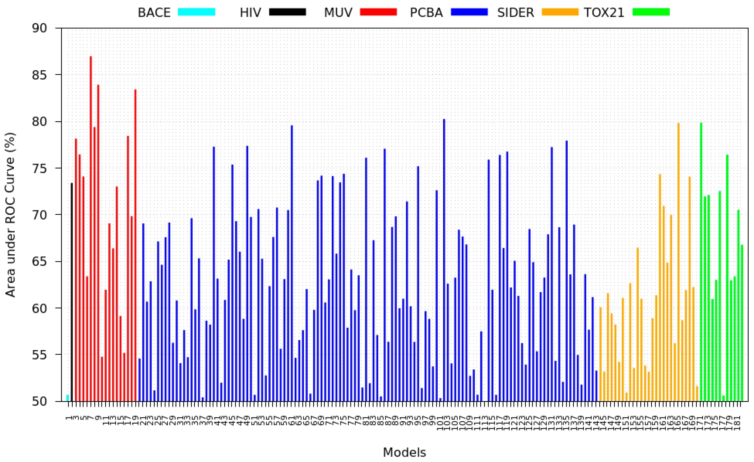
One final approach to ranking prediction, which is proposed in this work, is to simply let the pre-trained model classify the target validation data without any fine-tuning, i.e., zero-shot inference. The intuition behind this approach closely follows that of the last two approaches. First, if the source dataset is similar to that of the target dataset, the model might perform better after fine-tuning. This similarity was tested in regards to the molecules in IDS, but is applied to the bio-activity labels in zero-shot inference. Second, if the model has learned to distinguish between active and inactive molecules of the target dataset, it might have a better performance after fine-tuning. The main difference to MSC is that now the ROC-AUC of predictions on the target validation dataset is used as a metric. This difference forces the knowledge learned within the last layer of the model to also be incorporated into the ranking metric, which was absent from the MSC method.

2.6. Evaluation

Performance of the models was evaluated using three different evaluation metrics, including accuracy rate, recall, and area under the Receiver Operation Characteristic curve (ROC-AUC). While accuracy is easily interpretable, it is not a good metric for a highly imbalanced dataset. On the other hand, ROC-AUC can demonstrate how well the model performs on both the majority and minority data distributions. Furthermore, the Boltzman-Enhanced Discrimination of the Receiver Operating Characteristic (BEDROC) is used as a performance metric [43]. This metric is often used in the molecular domain where datasets are commonly class imbalanced. Recall is used since it reflects how well the model is able to predict active molecules, and misclassifying the few active molecules in the dataset is a costly mistake in the field of drug discovery. For reproducibility purposes, all 182 trained models are provided.
Having acquired the three metrics for ranking models before fine-tuning, they are ranked in three different manners and compared to the ground truth ranking attained from fine-tuning on the target test set. In order to evaluate the ranking prediction, similar to [44], the correlation between the metrics and the improvement in ROC-AUC after transfer learning is calculated. Moreover, the number of accurate predictions between the top 10 models is recorded. Lastly, similar to [41], the Mean Reciprocal Ranking (MRR) is calculated for the predicted ranks, averaging on the top 10 predictions.

3. Results

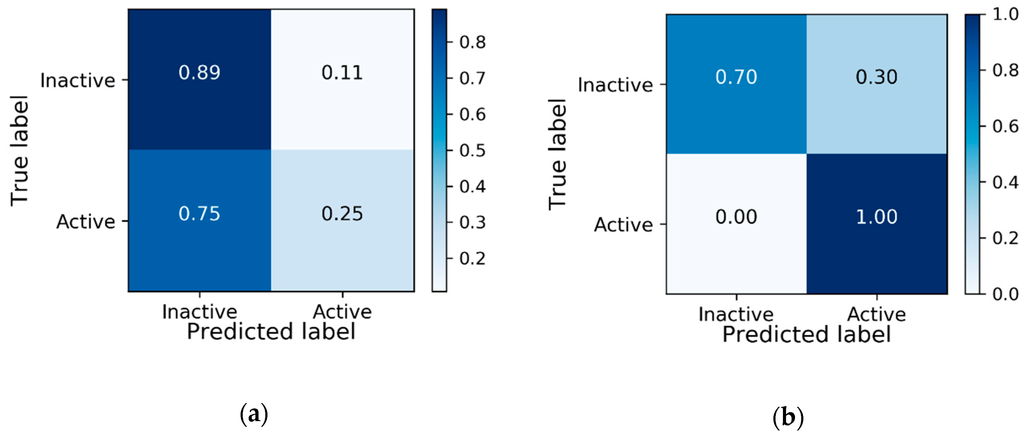
3.1. Baseline Model Results

The baseline model is trained on the target dataset for 30 epochs. The progress of the model is shown in Figure 2.
It is visible from Figure 2 that the model’s performance on train and validation sets start to diverge after the second epoch. This epoch is chosen as the optimum epoch and the results for this model are evaluated in Table 3.

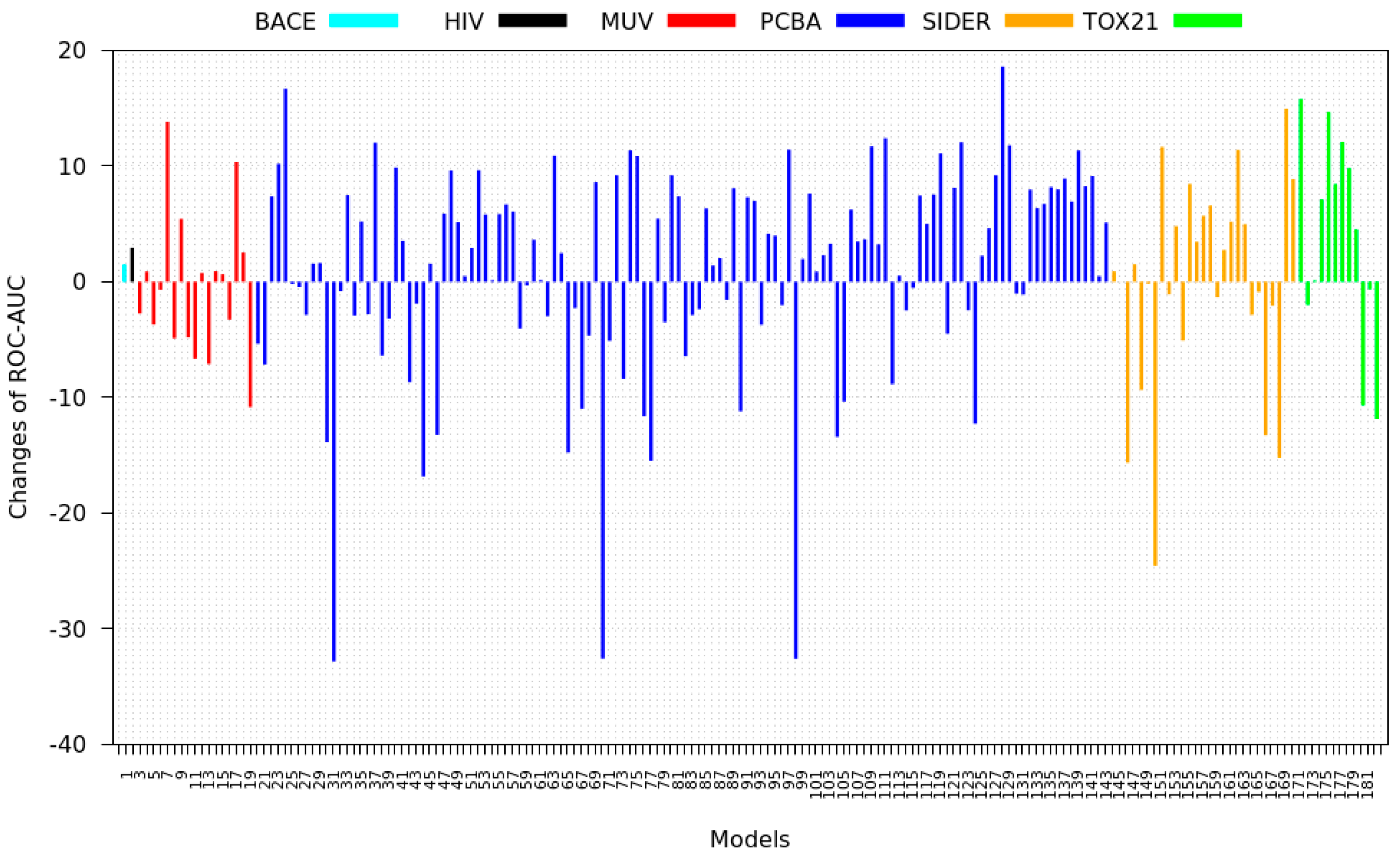
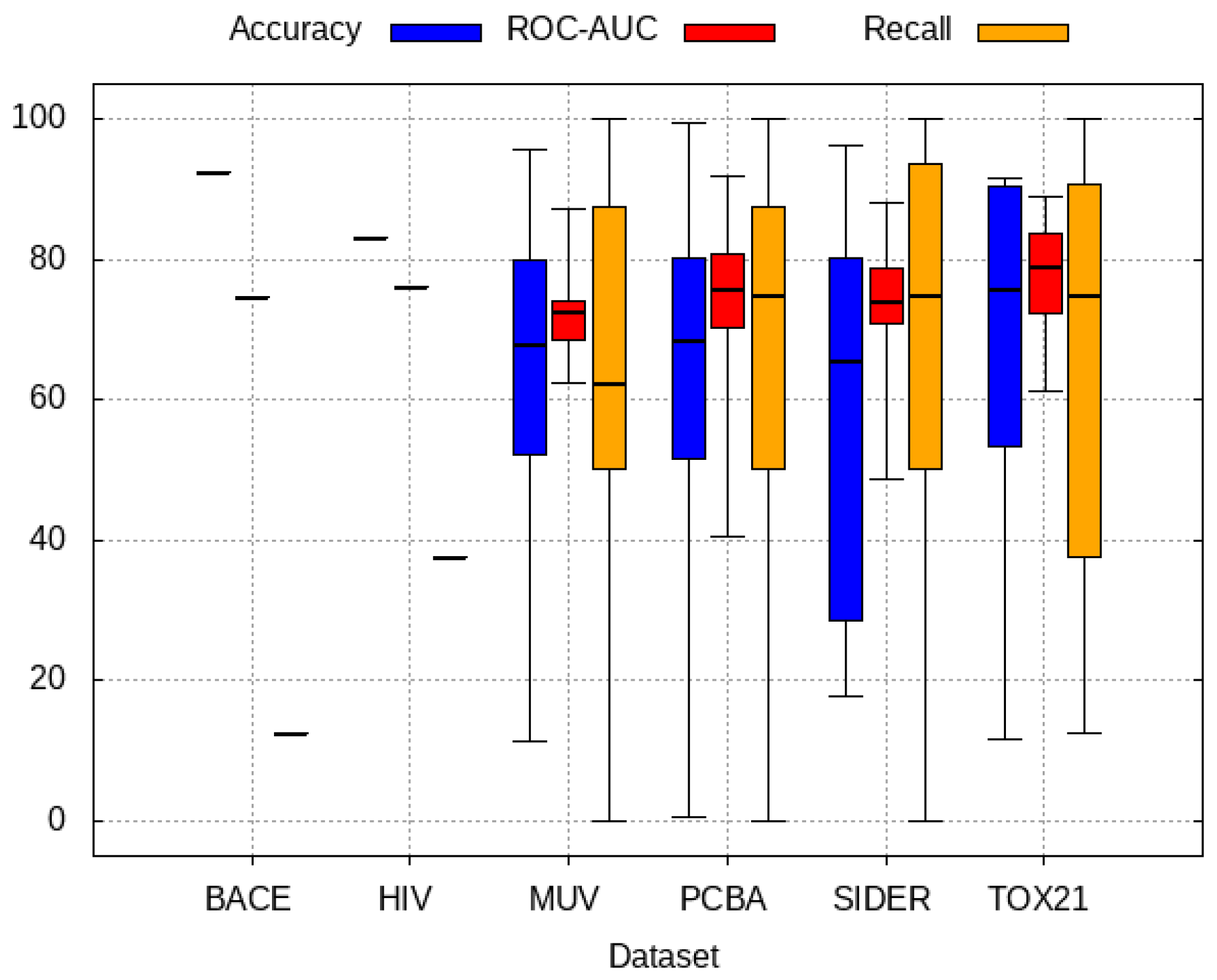
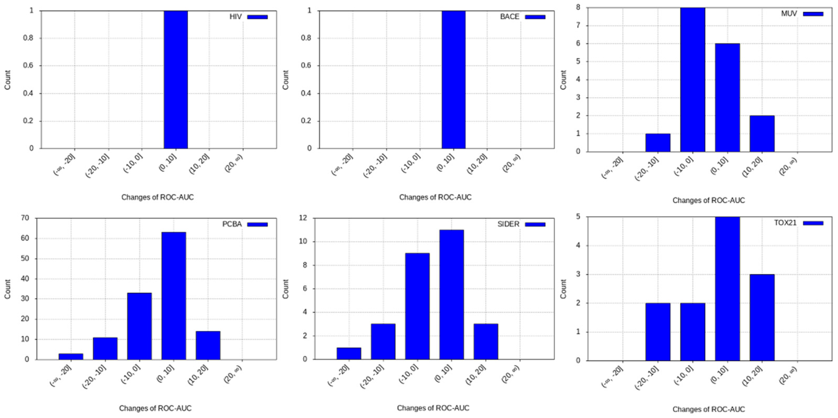
3.2. Transfer Learning Results

182 different source models from 6 datasets are trained for 30 epochs and then fine-tuned using the target dataset. The change in the ROC-AUC of the model on the target test set is depicted in Figure 3. These results can also be seen in further details in Appendix B (Figure A1).
As it is visible from Figure 3, models within the same datasets can either improve or worsen the performance of the target model. The average outcome of these models in regards to the source datasets are shown in Figure 4. The histogram of these results can be found in Appendix B (Figure A3).
Figure 4 demonstrates that on average, models transferred from the Tox21 dataset tend to perform well on the target task (highest average ROC-AUC), while the best and worst performing models originate from the PCBA dataset. The best performing models from each source task are shown in Table 4.
The overall best performing model is the model pre-trained on PCBA-651635 dataset and fine-tuned on the target dataset. This model also outperforms the state-of-the-art [18], which uses reinforcement learning from a related task to learn the target task. The best model’s confusion matrix is compared to the baseline model in Figure 5, showing noticeable improvement in correctly predicting bio-active molecules after transfer learning. The ROC curves for these two models can be viewed in Appendix B (Figure A2).

3.3. Inter-Dataset Similarity Results

The molecules within each source dataset are compared with those of the target dataset using Jaccard Index. The results are illustrated in Figure 6, showing that the Tox21 and SIDER datasets are the most different data from the target dataset, with PCBA and MUV having high similarities to the target dataset.

3.4. Mean Silhouette Coefficient Results

The target validation dataset is fed to the pre-trained models and deep features are extracted from the second to last layer. The MSC of these features between active and inactive clusters are shown in Figure 7, demonstrating that on average MUV has a higher capability of distinguishing between the target molecules. Moreover, PCBA contains tasks that possess the best and worst MSC scores.

3.5. Zero-Shot Inference Results

The target validation set is given to pre-trained models in order to be classified solely based on the knowledge gained from the source data and with no fine-tuning on the target data. The results are shown in Figure 8, demonstrating that MUV, Tox21, and PCBA are able to perform well on average through zero-shot inference.

3.6. Model Rank Prediction Results

After the results are acquired from three ranking approaches, the correlations between the results and the improvements in ROC-AUC of the test set are calculated. Furthermore, the number of correct top 10 predictions and their respective MRRs are calculated and reported in Table 5. IDS and MSC provided ranking predictions that were impractical for our target dataset. Zero-shot inference offers an improvement over previous approaches and can recommend two of the top ten models without performing fine-tuning.

4. Discussion and Results Interpretations

The baseline model for the target task shows clear signs of over-fitting at early stages of training, making it a prime candidate for performance improvement via better initialization. After transfer learning implementation, different initializations deliver varying performance and looking at three datasets in particular, enables better interpretation of the results:
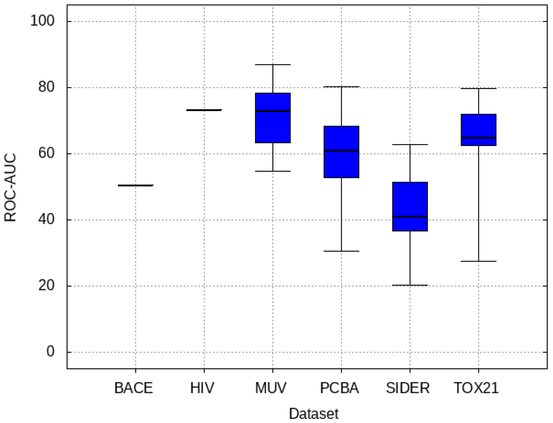
  • PCBA: This dataset is one of the closest and most similar (in terms of fingerprint similarity) to the target dataset. It has the highest MSC, indicating that deep features learned from this data source can distinguish between active and inactive molecules. The best performing data source belongs to this dataset. However, it also possesses the tasks that yielded the lowest MSC and the worst performance.
  • MUV: This dataset is also very similar to the target dataset. On average the models trained on this dataset delivered the highest MSC. However, on average these models yielded the lowest performance improvement.
  • Tox21: This dataset is the most dissimilar to the target dataset. It does not perform well when tested with MSC measurement. However, the models from this dataset deliver the highest average improvement after transfer learning.
From the cheminformatics point of view, these results demonstrate the insufficiency of molecular similarity and bio-activity clusterization for a performance’s prediction. In a non-structural, non-target-based virtual approach, the molecular data itself plays a very important role since there is no information regarding the target and its 3D structure. Therefore, similarity search and clustering would be a good approach to analyze data and to improve the performance. However, the first interpretation shows that a similarity search can even play an opposite role. In other words, the first interpretation is that judging by the training dataset or deep feature discrimination alone is not enough to understand the behavior of the model. These results demonstrate the fact that similar source dataset (to the target dataset) can perform poorly while dissimilar source datasets can give a high performance on average. Thus, refuting the traditional intuition that the source and target datasets should necessarily be similar. Deep feature discrimination did not prove to be fully capable of explaining the models’ behavior either, since models with the highest MSC still could perform rather poorly on the target dataset. This is aligned with the literature, since ranking prediction is still an unsolved task and the prediction accuracy of these approaches varies between datasets and is averaged at 7% [41].
The second interpretation is that zero-shot inference reveals more information from the model and the underlying training data, which in turn delivers a better understanding of the model’s behavior. The main difference between the proposed approach and the previous ones is examining how well the model can predict bio-activity of the molecules. Zero-shot inference includes information about target labels and the non-linearity of the last layer of the network into the ranking process, thus examining the model from more aspects. This can be seen in the fact that zero-shot inference offered better understanding of the Tox21 models’ behavior and a better perspective for inspecting the model.
It is also notable to mention that none of the three implemented approaches in this work could explain why the MUV dataset which has a high IDS, MSC, and zero-shot inference performance, still delivers the lowest average performance improvement after transfer learning. This fact demonstrates room for improvement in the ranking prediction models for future research. Further limitation of this work is viewing molecules as static inputs and not considering the flexibility of certain compounds.
The collection of pre-trained source models created in this work can be used as diverse initializations for future virtual screening tasks. The zero-shot inference approach provided in this work offers a better understanding of the pre-trained model and a more practical approach to rank the models before fine-tuning. Future directions for this research can include application of transfer learning within all datasets instead of one target dataset, inspection of learning based approaches for ranking prediction, or comparison of pre-trained model’s weight distribution to that of the baseline model.

5. Conclusions

Graph convolutional neural networks have improved the accuracy of virtual screening models, yet face the challenge of imbalanced, non-diverse, and small training datasets. In this work the TranScreen pipeline is designed and implemented to alleviate these challenges with the help of diverse weight initialization. Transfer learning is utilized from 182 source models trained on the MoleculeNet database. The models are then fine-tuned on an anticancer prediction task. The results show that some source models can significantly improve the performance of the baseline target model, with the best model achieving 0.92 ROC-AUC and 100% recall. A collection of the pre-trained models is curated and made available for future virtual screening tasks to be used as weight initialization. Moreover, three approaches are implemented to rank and recommend pre-trained models for a given task, which also gave insight to how the models behave in regards with the training data and feature representations. The code and pre-trained models created in this work are made accessible online through www.transilico.com.

Author Contributions

Conceptualization M.S.; methodology, M.S., A.K.; implementation and visualization, A.K.; data curation A.K.A.; formal analysis, M.S.; investigation, J.W.; writing—original draft preparation, M.S.; writing—review and editing, J.W.; supervision and project administration, J.-S.Y. All authors have read and agreed to the published version of the manuscript.

Funding

This research received no external funding.

Conflicts of Interest

The authors declare no conflicts of interest.

Appendix A

Cancer and p53

Cancer is a leading cause of death globally, ranking first or second for deaths in ages below 70 in the majority of countries [45]. This predominant contribution to global mortality, in addition to a significant economic burden [46], places cancer research in a place of paramount importance. In essence, the term “cancer” refers to a family of diseases that arise from abnormal cell growth; this abnormal growth occurs as a result of several cellular changes, usually triggered by mutations in the genome. At their root, many mutations and epigenetic changes can be traced to lifestyle and environmental factors, such as the use of tobacco products, alcohol intake, diet, exercise, and exposure to carcinogens and radiation; still other cancers are the result of inherited mutations and infections. The formation of tumors is a multistep process, characterized by several cellular “hallmarks of cancer”, including sustained proliferative signaling, evasion of growth suppressors, resistance to cell death, enabled replicative immortality, induction of angiogenesis, and activation of invasion and metastasis; these characteristics are fueled by both genomic instability and inflammation [47]. The body employs several mechanisms to protect against cancer formation, known as “immunosurveillance”, while tumors also evolve to avoid detection and clearance, via immune evasion [48]. The threshold between benign and malignant tumors is defined by migration of the tumor cells to a different location in the body, known as metastasis; this transition involves dedifferentiation of the cells into a stem-like migratory phenotype, and is associated with complication of treatment [49]. Traditional cancer treatment strategies involve surgical removal of tumors, radiotherapy, hormone therapy, and chemotherapy, while newer approaches include immunotherapy and targeted therapies. Targeted therapy differs from traditional chemotherapy in that it focuses on cancer-specific molecules, rather than acting on general cellular processes [50].
One of the ways to view cancer on a cellular level is as an imbalance of oncogenes, which can promote cancer; and tumor-suppressor genes (TSG), which work to prevent it [51]. Mutations in TSGs can lead to inhibition of their normal cancer-surveilling activity, allowing tumorigenesis to go unchecked [52]. One of the most important TSGs is TP53, which encodes the p53 protein, sometimes referred to as the “guardian of the genome” [53]. P53 is activated in response to stressors like DNA damage and deregulated growth, which can lead to cancer if unaddressed; such signals activate sensors like ATM/ATR and ARF, respectively, which then activate p53 via phosphorylation [54]. Once activated, p53 acts as a transcription factor, inducing transcription of genes that facilitate DNA damage repair, entrance into senescence (dormancy), or cell-mediated death (apoptosis), removing the potential for tumor formation [55]. P53’s large role in tumor prevention can also be a weakness; cells with mutations in p53 are extremely vulnerable to transformation to a cancer state. Mutations in TP53 frequently interfere with p53’s DNA-binding activity in its role as a transcription factor [56]. Current approaches to cancer therapy that target p53 focus on restoration of wild-type p53 functionality, removal of mutant p53, and inhibition of downstream pathways of mutant p53 [57]. Loss of normal function allows damaged cells to proliferate and mutate further, contributing to tumor formation and metastasis [58]. Not all biomolecules enhancing the carcinogenicity after p53 loss of function are yet discovered. Consequently, it has been challenging to discover molecules with unknown target of interest as anticancer. One way to do so would be prediction using non-target-based models [27], which is the main approach taken in this work.

Appendix B

Figure A1. Detailed results of transfer learning from each source model after fine-tuning on the target dataset.
Bdcc 04 00016 g0a1
Figure A2. ROC-AUC curves on target test dataset for: (a) baseline model; (b) best performing model after transfer learning.
Bdcc 04 00016 g0a2
Figure A3. Histograms of the ROC-AUC improvements for each source model after fine-tuning on the target dataset.
Bdcc 04 00016 g0a3
Figure A4. Detailed similarity of each source dataset to the target dataset.
Bdcc 04 00016 g0a4
Figure A5. Discriminative capability (MSC) of each pre-trained source model in regards to the bio-activity of the target dataset’s molecules.
Bdcc 04 00016 g0a5
Figure A6. Detailed performance of pre-trained models inferring on target validation set without fine-tuning. (Correlation to improvement: 0.22)
Bdcc 04 00016 g0a6
Figure A7. Detailed performance of pre-trained models inferring on target validation set without fine-tuning, results smaller than 0.5 are flipped to be larger than 0.5. (Correlation to improvement: 0.08).
Bdcc 04 00016 g0a7
Table A1. Details of the common architecture and hyper-parameters.
ParameterValuesParameterValue
Number of conv. layers3Size of conv. layers64
Number of neurons256Learning rate0.0001
Dropout0Batch size128
Table A2. Source tasks and their referred number within the figures, part 1.
TaskNumberTaskNumberTaskNumberTaskNumber
BACE1PCBA-88536PCBA-48528171PCBA-588590106
HIV2PCBA-88737PCBA-48529072PCBA-588591107
MUV-4663PCBA-89138PCBA-48529473PCBA-588795108
MUV-7334PCBA-89939PCBA-48529774PCBA-588855109
MUV-7375PCBA-91240PCBA-48531375PCBA-602179110
MUV-8106PCBA-91441PCBA-48531476PCBA-1460111
MUV-8327PCBA-91542PCBA-48534177PCBA-602233112
MUV-8468PCBA-147943PCBA-145478PCBA-602310113
MUV-8529PCBA-92544PCBA-48534979PCBA-602313114
MUV-85810PCBA-92645PCBA-48535380PCBA-602332115
MUV-85911PCBA-92746PCBA-48536081PCBA-624170116
MUV-54812PCBA-93847PCBA-48536482PCBA-624171117
MUV-60013PCBA-99548PCBA-48536783PCBA-624173118
MUV-64414PCBA-163149PCBA-49294784PCBA-624202119
MUV-65215PCBA-163450PCBA-49320885PCBA-624246120
MUV-68916PCBA-168851PCBA-50432786PCBA-624287121
MUV-69217PCBA-172152PCBA-50433287PCBA-1461122
MUV-71218PCBA-210053PCBA-50433388PCBA-624288123
MUV-71319PCBA-210154PCBA-145789PCBA-624291124
PCBA-103020PCBA-214755PCBA-50433990PCBA-624296125
PCBA-146921PCBA-137956PCBA-50444491PCBA-624297126
PCBA-72055322PCBA-224257PCBA-50446692PCBA-624417127
PCBA-72057923PCBA-232658PCBA-50446793PCBA-651635128
PCBA-72058024PCBA-245159PCBA-50470694PCBA-651644129
PCBA-72070725PCBA-251760PCBA-50484295PCBA-651768130
PCBA-72070826PCBA-252861PCBA-50484596PCBA-651965131
PCBA-72070927PCBA-254662PCBA-50484797PCBA-652025132
PCBA-72071128PCBA-254963PCBA-50489198PCBA-1468133
PCBA-74325529PCBA-255164PCBA-54027699PCBA-652104134
PCBA-74326630PCBA-266265PCBA-1458100PCBA-652105135
PCBA-87531PCBA-267566PCBA-540317101PCBA-652106136
PCBA-147132PCBA-145267PCBA-588342102PCBA-686970137
PCBA-88133PCBA-267668PCBA-588453103PCBA-686978138
PCBA-88334PCBA-41169PCBA-588456104PCBA-686979139
PCBA-88435PCBA-46325470PCBA-588579105PCBA-720504140
Table A3. Source tasks and their referred number within the figures, part 2.
TaskNumberTaskNumberTaskNumberTaskNumber
PCBA-720532141Metabolism and nutrition disorders152Vascular disorders163SR-p53174
PCBA-720542142Musculoskeletal and connective tissue disorders153“Neoplasms benign, malignant and unspecified (incl cysts and polyps)”164NR-AR175
PCBA-720551143Nervous system disorders154“Pregnancy, puerperium and perinatal conditions”165NR-AR-LBD176
“Congenital, familial and genetic disorders”144“Injury, poisoning and procedural complications”155“Respiratory, thoracic and mediastinal disorders”166NR-Aromatase177
Eye disorders145Product issues156Blood and lymphatic system disorders167NR-ER178
Gastrointestinal disorders146Psychiatric disorders157Cardiac disorders168NR-ER-LBD179
General disorders and administration site conditions147Renal and urinary disorders158Ear and labyrinth disorders169NR-PPAR-gamma180
Hepatobiliary disorders148Reproductive system and breast disorders159Endocrine disorders170SR-ARE181
Immune system disorders149Skin and subcutaneous tissue disorders160NR-AhR171SR-ATAD5182
Infections and infestations150Social circumstances161SR-HSE172
Investigations151Surgical and medical procedures162SR-MMP173

References

  1. Carnero, A. High throughput screening in drug discovery. Clin. Transl. Oncol. 2006, 8, 482–490. [Google Scholar] [CrossRef] [PubMed]
  2. Mohs, R.C.; Greig, N.H. Drug discovery and development: Role of basic biological research. Alzheimer’s Dement. (N. Y.) 2017, 3, 651–657. (In English) [Google Scholar] [CrossRef] [PubMed]
  3. Miljković, F.; Rodríguez-Pérez, R.; Bajorath, J. Machine Learning Models for Accurate Prediction of Kinase Inhibitors with Different Binding Modes. J. Med. Chem. 2019. [Google Scholar] [CrossRef] [PubMed]
  4. Sánchez-Rodríguez, A.; Pérez-Castillo, Y.; Schürer, S.C.; Nicolotti, O.; Mangiatordi, G.F.; Borges, F.; Cordeiro, M.N.D.; Tejera, E.; Medina-Franco, J.L.; Cruz-Monteagudo, M. From flamingo dance to (desirable) drug discovery: A nature-inspired approach. Drug Discov. Today 2017, 22, 1489–1502. [Google Scholar]
  5. Cruz-Monteagudo, M.; Ancede-Gallardo, E.; Jorge, M.; Cordeiro, M.N.D.S. Chemoinformatics Profiling of Ionic Liquids—Automatic and Chemically Interpretable Cytotoxicity Profiling, Virtual Screening, and Cytotoxicophore Identification. Toxicol. Sci. 2013, 136, 548–565. [Google Scholar] [CrossRef] [Green Version]
  6. Perez-Castillo, Y.; Sánchez-Rodríguez, A.; Tejera, E.; Cruz-Monteagudo, M.; Borges, F.; Cordeiro, M.N.D.; Le-Thi-Thu, H.; Pham-The, H. A desirability-based multi objective approach for the virtual screening discovery of broad-spectrum anti-gastric cancer agents. PLoS ONE 2018, 13, e0192176. [Google Scholar] [CrossRef] [Green Version]
  7. Korotcov, A.; Tkachenko, V.; Russo, D.P.; Ekins, S. Comparison of Deep Learning With Multiple Machine Learning Methods and Metrics Using Diverse Drug Discovery Data Sets. Mol. Pharm. 2017, 14, 4462–4475. [Google Scholar] [CrossRef]
  8. Popova, M.; Isayev, O.; Tropsha, A. Deep reinforcement learning for de novo drug design. Sci. Adv. 2018, 4, eaap7885. [Google Scholar] [CrossRef] [Green Version]
  9. Minnich, A.J.; McLoughlin, K.; Tse, M.; Deng, J.; Weber, A.; Murad, N.; Madej, B.D.; Ramsundar, B.; Rush, T.; Calad-Thomson, S.; et al. AMPL: A Data-Driven Modeling Pipeline for Drug Discovery. J. Chem. Inf. Model. 2020, 60, 1955–1968. [Google Scholar] [CrossRef]
  10. Kearnes, S.; McCloskey, K.; Berndl, M.; Pande, V.; Riley, P. Molecular graph convolutions: Moving beyond fingerprints. J. Comput. Aided Mol. Des. 2016, 30, 595–608. [Google Scholar] [CrossRef] [Green Version]
  11. Gimeno, A.; Ojeda-Montes, M.J.; Tomás-Hernández, S.; Cereto-Massagué, A.; Beltrán-Debón, R.; Mulero, M.; Pujadas, G.; Garcia-Vallvé, S. The Light and Dark Sides of Virtual Screening: What Is There to Know? Int. J. Mol. Sci. 2019, 20, 1375. [Google Scholar] [CrossRef] [PubMed] [Green Version]
  12. Pérez-Sianes, J.; Pérez-Sánchez, H.; Díaz, F. Virtual Screening: A Challenge for Deep Learning. In 10th International Conference on Practical Applications of Computational Biology & Bioinformatics; Springer International Publishing: Cham, Switzerland, 2016; pp. 13–22. [Google Scholar]
  13. Fischer, B.; Merlitz, H.; Wenzel, W. Increasing Diversity in In-silico Screening with Target Flexibility. In Computational Life Sciences; Springer: Berlin/Heidelberg, Germany, 2005; pp. 186–197. [Google Scholar]
  14. Hert, J.; Willett, P.; Wilton, D.J.; Acklin, P.; Azzaoui, K.; Jacoby, E.; Schuffenhauer, A. Comparison of Fingerprint-Based Methods for Virtual Screening Using Multiple Bioactive Reference Structures. J. Chem. Inf. Comput. Sci. 2004, 44, 1177–1185. [Google Scholar] [CrossRef] [PubMed]
  15. Ramsundar, B.; Kearnes, S.; Riley, P.; Webster, D.; Konerding, D.; Pande, V. Massively multitask networks for drug discovery. arXiv 2015, arXiv:1502.02072. [Google Scholar]
  16. Altae-Tran, H.; Ramsundar, B.; Pappu, A.S.; Pande, V. Low Data Drug Discovery with One-Shot Learning. ACS Cent. Sci. 2017, 3, 283–293. [Google Scholar] [CrossRef]
  17. Hu, W.; Liu, B.; Gomes, J.; Zitnik, M.; Liang, P.; Pande, V.; Leskovec, J. Strategies for Pre-training graph neural networks. arXiv 2019, arXiv:1905.12265. [Google Scholar]
  18. Liu, S. Exploration on Deep Drug Discovery: Representation and Learning; Computer Science, University of Wisconsin-Madison: Madison, WI, USA, 2018. [Google Scholar]
  19. Wu, Z.; Ramsundar, B.; Feinberg, E.N.; Gomes, J.; Geniesse, C.; Pappu, A.S.; Leswing, K.; Pande, V. MoleculeNet: A benchmark for molecular machine learning. Chem. Sci. 2018, 9, 513–530. [Google Scholar] [CrossRef] [Green Version]
  20. Baugh, E.H.; Ke, H.; Levine, A.J.; Bonneau, R.A.; Chan, C.S. Why are there hotspot mutations in the TP53 gene in human cancers? Cell Death Differ. 2018, 25, 154–160. [Google Scholar] [CrossRef]
  21. PubChem Database. Source=NCGC AID=904. 2007. Available online: https://pubchem.ncbi.nlm.nih.gov/bioassay/904 (accessed on 18 May 2020).
  22. Rogers, D.; Hahn, M. Extended-Connectivity Fingerprints. J. Chem. Inf. Model. 2010, 50, 742–754. [Google Scholar] [CrossRef]
  23. Torng, W.; Altman, R.B. Graph Convolutional Neural Networks for Predicting Drug-Target Interactions. J. Chem. Inf. Model. 2019, 59, 4131–4149. [Google Scholar] [CrossRef]
  24. Coley, C.W.; Jin, W.; Rogers, L.; Jamison, T.F.; Jaakkola, T.S.; Green, W.H.; Barzilay, R.; Jensen, K.F. A graph-convolutional neural network model for the prediction of chemical reactivity. Chem. Sci. 2019, 10, 370–377. [Google Scholar] [CrossRef] [Green Version]
  25. Ramsundar, B.; Eastman, P.; Walters, P.; Pande, V.; Leswing, K.; Wu, Z. Deep Learning for the Life Sciences; O’Reilly Media: Sebastopol, CA, USA, 2019. [Google Scholar]
  26. Bjerrum, E.J. Smiles enumeration as data augmentation for neural network modeling of molecules. arXiv 2017, arXiv:1703.07076. [Google Scholar]
  27. Arshadi, A.K.; Salem, M.; Collins, J.; Yuan, J.S.; Chakrabarti, D. DeepMalaria: Artificial Intelligence Driven Discovery of Potent Antiplasmodials. Front. Pharmacol. 2019, 10, 1526. [Google Scholar] [CrossRef] [PubMed] [Green Version]
  28. Devlin, J.; Chang, M.-W.; Lee, K.; Toutanova, K. Bert: Pre-training of deep bidirectional transformers for language understanding. arXiv 2018, arXiv:1810.04805. [Google Scholar]
  29. Nassif, A.B.; Shahin, I.; Attili, I.; Azzeh, M.; Shaalan, K. Speech Recognition Using Deep Neural Networks: A Systematic Review. IEEE Access 2019, 7, 19143–19165. [Google Scholar] [CrossRef]
  30. Boumi, S.; Vela, A.; Chini, J. Quantifying the relationship between student enrollment patterns and student performance. arXiv 2020, arXiv:2003.10874. [Google Scholar]
  31. Zhang, K.; Guo, Y.; Wang, X.; Yuan, J.; Ding, Q. Multiple Feature Reweight DenseNet for Image Classification. IEEE Access 2019, 7, 9872–9880. [Google Scholar] [CrossRef]
  32. Sun, Q.; Liu, Y.; Chua, T.-S.; Schiele, B. Meta-transfer learning for few-shot learning. In Proceedings of the IEEE Conference on Computer Vision and Pattern Recognition, Long Beach, CA, USA, 16–20 June 2019; pp. 403–412. [Google Scholar]
  33. Liu, S.; Johns, E.; Davison, A.J. End-to-end multi-task learning with attention. In Proceedings of the IEEE Conference on Computer Vision and Pattern Recognition, Long Beach, CA, USA, 16–20 June 2019; pp. 1871–1880. [Google Scholar]
  34. Zhuang, F.; Qi, Z.; Duan, K.; Xi, D.; Zhu, Y.; Zhu, H.; Xiong, H.; He, Q. A Comprehensive Survey on Transfer Learning. arXiv 2019, arXiv:1911.02685. [Google Scholar]
  35. Frankle, J.; Carbin, M. The lottery ticket hypothesis: Finding sparse trainable neural networks. arXiv 2018, arXiv:1803.03635. [Google Scholar]
  36. Fawaz, H.I.; Forestier, G.; Weber, J.; Idoumghar, L.; Muller, P. Transfer learning for time series classification. In Proceedings of the 2018 IEEE International Conference on Big Data (Big Data), Zurich, Switzerland Seattle, WA, USA, 10–13 December 2018; pp. 1367–1376. [Google Scholar]
  37. Wang, M.; Deng, W. Deep visual domain adaptation: A survey. Neurocomputing 2018, 312, 135–153. [Google Scholar] [CrossRef] [Green Version]
  38. Zhang, H.; Koniusz, P. Model Selection for Generalized Zero-Shot Learning. In Computer Vision—ECCV 2018 Workshops; Springer International Publishing: Cham, Switzerland, 2019; pp. 198–204. [Google Scholar]
  39. Zhang, H.; Koniusz, P. Zero-Shot Kernel Learning. In Proceedings of the 2018 IEEE/CVF Conference on Computer Vision and Pattern Recognition, Salt Lake City, UT, USA, 18–22 June 2018; pp. 7670–7679. [Google Scholar]
  40. Ben-David, S.; Blitzer, J.; Crammer, K.; Pereira, F. Analysis of representations for domain adaptation. In Advances in NEURAL Information Processing Systems; The MIT Press: Cambridge, MA, USA, 2007; pp. 137–144. [Google Scholar]
  41. Meiseles, A.; Rokach, L. Source Model Selection for Deep Learning in the Time Series Domain. IEEE Access 2020, 8, 6190–6200. [Google Scholar] [CrossRef]
  42. Liu, S.; Alnammi, M.; Ericksen, S.S.; Voter, A.F.; Ananiev, G.E.; Keck, J.L.; Hoffmann, F.M.; Wildman, S.A.; Gitter, A. Practical Model Selection for Prospective Virtual Screening. J. Chem. Inf. Model. 2019, 59, 282–293. [Google Scholar] [CrossRef] [PubMed] [Green Version]
  43. Swamidass, S.J.; Azencott, C.-A.; Lin, T.-W.; Gramajo, H.; Tsai, S.-C.; Baldi, P. Influence relevance voting: An accurate and interpretable virtual high throughput screening method. (in eng). J. Chem. Inf. Model. 2009, 49, 756–766. [Google Scholar] [CrossRef] [PubMed]
  44. Zhang, H.; Koniusz, P. Power Normalizing Second-Order Similarity Network for Few-Shot Learning. In Proceedings of the 2019 IEEE Winter Conference on Applications of Computer Vision (WACV), Waikoloa Village, HI, USA, 7–11 January 2019; pp. 1185–1193. [Google Scholar]
  45. Bray, F.; Ferlay, J.; Soerjomataram, I.; Siegel, R.L.; Torre, L.A.; Jemal, A. Global cancer statistics 2018: GLOBOCAN estimates of incidence and mortality worldwide for 36 cancers in 185 countries. CA Cancer J. Clin. 2018, 68, 394–424. [Google Scholar] [CrossRef] [PubMed] [Green Version]
  46. Yabroff, K.R.; Warren, J.L.; Brown, M.L. Costs of cancer care in the USA: A descriptive review. Nat. Clin. Pract. Oncol. 2007, 4, 643–656. [Google Scholar] [CrossRef]
  47. Hanahan, D.; Weinberg, R.A. Hallmarks of cancer: The next generation. Cell 2011, 144, 646–674. [Google Scholar] [CrossRef] [Green Version]
  48. Smyth, M.J.; Dunn, G.P.; Schreiber, R.D. Cancer immunosurveillance and immunoediting: The roles of immunity in suppressing tumor development and shaping tumor immunogenicity. Adv. Immunol. 2006, 90, 1–50. [Google Scholar]
  49. Brabletz, T.; Jung, A.; Spaderna, S.; Hlubek, F.; Kirchner, T. Opinion: Migrating cancer stem cells—An integrated concept of malignant tumour progression. Nat. Rev. Cancer 2005, 5, 744–749. [Google Scholar] [CrossRef]
  50. Huang, M.; Shen, A.; Ding, J.; Geng, M. Molecularly targeted cancer therapy: Some lessons from the past decade. Trends Pharmacol. Sci. 2014, 35, 41–50. [Google Scholar] [CrossRef]
  51. Croce, C.M. Oncogenes and cancer. N. Engl. J. Med. 2008, 358, 502–511. [Google Scholar] [CrossRef] [Green Version]
  52. Wang, L.H.; Wu, C.F.; Rajasekaran, N.; Shin, Y.K. Loss of Tumor Suppressor Gene Function in Human Cancer: An Overview. Cell Physiol. Biochem. 2018, 51, 2647–2693. [Google Scholar] [CrossRef]
  53. Lane, D.P. Cancer. p53, guardian of the genome. Nature 1992, 358, 15–16. [Google Scholar] [CrossRef]
  54. Ashcroft, M.; Taya, Y.; Vousden, K.H. Stress signals utilize multiple pathways to stabilize p53. Mol. Cell Biol. 2000, 20, 3224–3233. [Google Scholar] [CrossRef] [PubMed] [Green Version]
  55. Oren, M. Decision making by p53: Life, death and cancer. Cell Death Differ. 2003, 10, 431–442. [Google Scholar] [CrossRef] [PubMed]
  56. Goh, A.M.; Coffill, C.R.; Lane, D.P. The role of mutant p53 in human cancer. J. Pathol. 2011, 223, 116–126. [Google Scholar] [CrossRef] [PubMed]
  57. Parrales, A.; Iwakuma, T. Targeting Oncogenic Mutant p53 for Cancer Therapy. Front. Oncol. 2015, 5, 288. [Google Scholar] [CrossRef] [Green Version]
  58. Powell, E.; Piwnica-Worms, D.; Piwnica-Worms, H. Contribution of p53 to metastasis. Cancer Discov. 2014, 4, 405–414. [Google Scholar] [CrossRef] [Green Version]
Figure 1. The overview of the TranScreen Pipeline. A common network architecture is determined and used to train multiple source models. The pre-trained models are fine-tuned on the target dataset. Three approaches are implemented to predict how well these pre-trained models can perform on the target task before fine-tuning.
Bdcc 04 00016 g001
Figure 2. Performance on training and validation sets at each epoch for the target’s baseline model.
Bdcc 04 00016 g002
Figure 3. The change in performance and the area under receiver operating curve (ROC-AUC) of model after transfer learning.
Bdcc 04 00016 g003
Figure 4. The average change in performance and ROC-AUC of after transfer learning from each dataset.
Bdcc 04 00016 g004
Figure 5. Confusion matrix comparison between: (a) baseline model; (b) best performing model after transfer learning.
Bdcc 04 00016 g005
Figure 6. Similarity between each source dataset and the target dataset. Higher Jaccard Index indicates higher degree of similarity between the molecules.
Bdcc 04 00016 g006
Figure 7. Mean Silhouette Coefficient (MSC) between each source dataset and target datasets. Higher MSC indicates more distinguishable clusters formed from bio-active and inactive molecules.
Bdcc 04 00016 g007
Figure 8. Performance of pre-trained models inferring on target validation set without fine-tuning. Higher ROC-AUC indicates better zero-shot inference.
Bdcc 04 00016 g008
Table 1. Source data information.
DatasetData TypeNumber of TasksNumber of Compounds
PCBASMILES124437,929
MUV1793,087
HIV141,127
BACE11513
Tox21127831
SIDER271427
Table 2. Target data information.
DatasetData TypeNumber of TasksNumber of CompoundsNumber of Active Compounds
PCBA-904SMILES1437,929528
Table 3. Baseline results for the cancer candidate prediction models.
TaskPartitionAccuracyRecallROC-AUC
PCBA-904Validation90.9657.140.7846
PCBA-904Test89.66250.7322
Table 4. Best performing source models for transfer learning on the target test dataset.
Source DatasetSource TaskTarget TaskAccuracyRecallBEDROC (Alpha = 1)ROC-AUCImprovement
PCBAPCBA-651635PCBA-90471.481000.7790.9180.186
Tox21NR-AhR82.11750.6780.8890.158
SIDEREar and labyrinth disorders73.5687.50.3920.8820.150
MUVMUV-83281.68750.6770.8710.138
HIVHIV83.0537.50.5050.7610.029
BACEBACE92.3112.50.3990.7470.015
PCBA [18]PCBA-903---0.81-
Table 5. Evaluation of each pre-trained model ranking approach.
Ranking ApproachCorrelation to ImprovementMRR (Top 10)Correct Predictions (Top 10)
IDS [36]−0.030.0170
MSC [41]0.050.0090
Zero-Shot (Ours)0.220.0632

