Abstract
Agent-based modelling is a successful technique in many different fields of science. As a bottom-up method, it is able to simulate complex behaviour based on simple rules and show results at both micro and macro scales. However, developing agent-based models is not always straightforward. The most difficult step is defining the rules for the agent behaviour, since one often has to rely on many simplifications and assumptions in order to describe the complicated decision making processes. In this paper, we investigate the idea of building a framework for agent-based modelling that relies on an artificial neural network to depict the decision process of the agents. As a proof of principle, we use this framework to reproduce Schelling’s segregation model. We show that it is possible to use the presented framework to derive an agent-based model without the need of manually defining rules for agent behaviour. Beyond reproducing Schelling’s model, we show expansions that are possible due to the framework, such as training the agents in a different environment, which leads to different agent behaviour.
1. Introduction
The main idea behind agent-based modelling [1] is to describe a system by using its constituent parts as a starting point. These so-called “agents” have certain properties and actions available to them and the whole system is then modelled based on the actions and interactions of the agents. Thus, the dynamic in this bottom-up approach originates at the micro scale, in contrast to most macroscopic modelling approaches, where the dynamic is mostly governed by equations that describe system properties. Agent-based modelling is relevant for different scientific disciplines, in which systems can be seen as comprised of a large number of interacting entities. There are many examples of areas where agent-based modelling was used successfully: for evacuation models [2], it is quite intuitive to describe the system as interacting agents. The goal of each agent is clear, but due to their interactions interesting effects can emerge. Another important area for agent-based models are traffic simulations [3,4,5]. The goals of the agents are also clear here (getting from one point to an other point), but, due to interactions with other agents, they must behave differently from how they would if they could use all roads for themselves, leading to congestion or even stop-and-go traffic. Somewhat related to this field is the field of city planning [6], where models with mobile agents, which have various needs, can give crucial input about how efficient a specific plan for a city is. Beyond that, there are also various applications in social sciences [7,8] and the simulation of human systems [9]. In the fields of ecology [10] and complexity research [11], agent-based models can also be used. Another important application of agent-based modelling is computational economics [12]. This field is especially active and it is possible to simulate whole economies from the bottom up [13,14,15,16]. An agent-based approach can also be used if one is interested in (social) networks [17] and phenomena that are influenced by network effects. A prominent example would be tax compliance and tax evasion [18], which can be better understood by models that see this behaviour not as a external feature of the system, but as something that emerges on the agent-level and is disseminated via a network.
For the development of each agent-based model certain steps are necessary: (i) defining the agents; (ii) defining the environment; (iii) defining what agents know and sense; (iv) defining the goal of the agents; and (v) finding rules for their behaviour. While the first four steps are relatively straightforward for most models, the last step features some unique challenges. The rules should use the information the agents have access to as an input and yield what action they take in this situation as an output, considering bounded rationality [19]. The input that the agents use for their decision is relatively easy to find and to justify. In an evacuation model for example, agents sense their immediate surroundings and choose their path accordingly, but they have no information about the situation behind a visual barrier such as a wall. In a traffic model, agents know which roads are usually congested and which are not and may have access to information about recent construction sites or accidents and mainly base their path decision on this input. However, specifying the rules that lead to a decision is much more difficult and often relies on assumptions from psychology or economics, which are often hard to back up empirically or by theories. This makes the search for valid rules for agent behaviour one of the biggest challenges in agent-based modelling [20].
In this paper, a framework is presented that uses an artificial neural network to simulate the decision making process in an agent-based model. The framework is generic enough that it can be used for any kind of agent-based model, since the training of the artificial neural network is included in the process and therefore independent of the investigated system or model. The framework is related to reinforcement learning [21,22], but there are important differences. While the goal of reinforcement learning is to arrive at an optimal solution, the framework focuses on providing a realistic decision process, by training agents in realistic environments and not in hypothetical environments proven to show the best results, as is done for reinforcement learning. This also includes the possibility of wrong decisions or misjudgement, allowing us to model a wide range of systems, in which agents are not able to find the optimal solution, realistically.
This paper is organised as follows. Section 2 details the used methods. Section 2.1 gives a short introduction to artificial neural networks. A detailed description of the proposed framework can be found in Section 2.2. As a proof of principle, the framework is applied to reproduce Schelling’s famous segregation model [23,24] in Section 2.3. Results of this application are presented in Section 3. Section 4 discusses these results. Finally, Section 5 gives a short conclusion of this study.
2. Methods
The core idea of the presented framework is to replace the manual definition of rules that govern agent behaviour by an automated, generic process. This shifts the effort during model development away from finding rules that correctly depict reality towards defining an equation for a score or a utility function for an agent. This utility function can be tailored specifically to model the investigated system and it is also possible to use different utility functions for different agents. In most cases, the definition of a utility function will be a simpler and less subjective task than finding rules for behaviour. The actual decision making, i.e. the decision on what action to perform given the current sensory input and past experience, is then handled by an artificial neural network. A simple example where this advantage is evident would be an agent-based model that describes a game of chess. Both players want to win the game, so their utility function would be trivial to find:
However, finding a rule based description of which moves the players think will lead them to maximise this function is virtually impossible. A neural network can close this gap.
2.1. Artificial Neural Networks
Artificial neural networks [25,26,27,28] are based on the idea of building artificial networks that closely resemble the principles of biological neural networks. A signal enters the network through some sensory cells or input nodes and is transferred to a complex network. Depending on the individual connections between nodes, this input signal is then transformed into an output at an output node (see Figure 1). Similar to a biological neural network, an artificial neural network also needs to be trained. This means it needs to be confronted with various input signals and receive feedback regarding the desired output, so that the required connections can be formed. There are various techniques to train artificial neural networks with different benefits and downsides [29,30,31,32,33,34,35], but they all have in common that they rely on a large amount of data, either measured or generated.
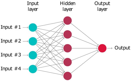
Figure 1.
Schematic depiction of a neural network: A signal enters the input layer. A complex network then transforms it into an output. Optimising the network by changing the connections between the nodes, so that it always produces the desired outcome, is called training.
Trained neural networks can then be used for many applications, such as data processing [36], function approximation [37], solving prediction problems [38] and solving classification problems [39]. In a classification problem, a neural network is presented with certain inputs (images or other data) and has to classify each input as a member of a set of predefined categories or classes. The most prominent example for a neural network that solves a classification problem is the automated reading of handwriting. The inputs are images of handwritten letters and each of them corresponds to an actual letter. In that case, the input layer of the network would encode the image and the output layer would have one node for each letter in the alphabet. Using images that are already classified, the network can then be trained to produce a signal in the correct output node.
For the framework, we focus on the classification problem, since this is the problem agents are faced with. They have a set of possible actions available to them and need to decide for each whether this would be a good or a bad decision in their current situation. Alternatively, this could be framed as a prediction problem. In a prediction problem, agents would not classify decision as good or bad but would try to approximate the utility that this decision would lead to. Thus, they would search for a quantitative value for each possible decision and not for a qualitative one, making the process more complicated. Furthermore, the formulation as a prediction problem would assume that agents have a quantitative understanding of their utility function. Since this assumption is unjustified in many systems, the basis of our framework is the aforementioned classification problem, where a qualitative understanding (worse, the same, or better) of their utility is sufficient.
2.2. A Framework for Agent-Based Modelling
The core of the presented framework is a trained artificial neural network that solves the following classification problem: “Which of the actions available to me can increase my score?” To train the network, we first need to gather a sufficient amount of data. Each entry should consist of the sensory input of the agent, the decision it made and whether this decision increased its score or not. The modelling process is split into two parts: the experience phase, in which agents make random decisions in order gather experience data, and the application phase, in which the agents use the trained neural network to make realistic decisions. These two phases are depicted schematically in Figure 2.
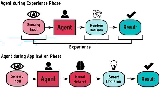
Figure 2.
Agents are trained by making random decisions and storing the achieved result as experience. During the application phase, a neural network is used for decision making.
During the experience phase, agents are initialised (in general) in the same environment and under the same conditions in which the actual modelling will take place. Agents take turns and perform the following steps in each turn:
- Save all the sensory inputs in a vector .
- Calculate current score from utility function and save as .
- Perform a random action a from the list of available actions.
- Calculate the new score and save as .
- Rate the decision and save as r: good if , bad otherwise.
- Add an entry to the experience database: .
After the experience phase, we end up with a large database that contains information about whether a certain action in a certain situation can be classified as good or bad. Similar to the problem of reading handwritten letters, this information of correctly classified inputs can be used to train the neural network, so that it can then classify inputs, even though they are not exactly the same as the ones it trained with. When applying a neural network for this purpose, one has to take great care regarding validation: Validating a neural network that is used for reinforcement learning is simple. The closer the rate of correct classifications is to 100%, the better. Here, the situation is more complicated: We do not want perfect, but realistic decisions. Thus, reaching a correct classification rate of close to 100% cannot be used as an indicator for successful training. For our application, one has to look at convergence: If the rate of correct classifications stops improving, this is a sign that the agents are sufficiently trained, even if the only reach a rate of, e.g., 60%.
After the training of the neural network, the application phase begins. Agents are reinitialised, so that the random decisions they took during training have no influence on their state. In addition, in the application phase the agents take turns and perform the following steps:
- Save all the sensory inputs in a vector .
- For each action available action , use as an input for the neural network.
- Rank all actions according to the certainty that they are good decisions.
- Perform the action which was ranked highest.
2.3. Applying the Framework
To showcase the presented framework, we apply it to the well-know segregation model by Schelling [23,24]. Agents are distributed randomly on a grid (see Figure 3). Each agent is a member of one of two groups. Every time step, agents can choose to stay at their position or move to a random unoccupied place on the grid. In the original model, one has to define a certain percentage of neighbours from the other group, above which the agents should move away. Depending on this value, one can observe weak or strong segregation [40]. Using the presented framework, there is no need to determine such specific rules. We simply define how to calculate a score S: Agents gain a point for every neighbour in the same group and lose a point for every neighbour in the other group:
with being the score of the agent at position , and being the group membership of the agent (1 for membersr of Group 1, for members of Group 2 and 0 for unoccupied cells). The first term of Equation (2) counteracts the contribution of the sums, where and an agent would be awarded a point for being its own neighbour. Note that the actual formulation of this equation has no impact on the results, as long as each “correct” neighbour increases the score and each “incorrect” neighbour decreases the score by the same amount. Having different weights for positive and negative contributions is possible, but seems counter-intuitive in the context of segregation [41].
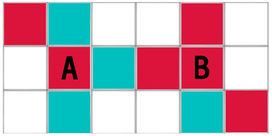
Figure 3.
A sample grid with agents: Agent A has one fitting neighbour (top left) and three neighbours, which are members of the other group. Agent B has three fitting neighbours and one of the other group.
In addition to this score, we have to define what agents can sense or know: In this implementation, we assume that agents know which group they are in and that they can see the group of all agents in their Moore neighbourhood [42]. These are all the assumptions that are required for the experience phase.
During the experience phase, agents make random decisions. They store their sensory input and their decision as a positive experience, if the score increased as an effect of the decision and as a negative experience if it decreased. Since the decisions of all agents are random, the states of the system are also more or less random. This means we need to collect data over long periods of time, in order to also have information about situations that have only a small probability of occurring randomly. However, since the data can be generated automatically and this process only involves a random decision, an action and the recalculation of the score, it is computationally cheap. For this study, we generated 1000 time steps in a system consisting of agents, leading to 200,000 experiences, which were used for training the neural network.
In the application phase, agents use the trained neural network in order to classify all possible actions as positive or negative and choose what they think is the best option. Note that in this phase the network will encounter data not seen before. Ideally, they should show patterns of segregation, similar to the original model. However, in the framework, we never defined any specific rules or equipped agents with the knowledge what the input parameters mean. The agents receive a vector containing numbers, but they do not know what information is encoded there or how it is encoded. They learn their meaning during the experience phase, which makes the framework highly flexible.
In addition to replicating the original model, we can also experiment with the experience phase. On the one hand, we can change the environment in which the agents train, so that it is different from the one the agents encounter during application. That way we can investigate any change in behaviour that comes from a different training environment. On the other hand, we can truncate some of the senses of the agents during training. This enables us to pinpoint which sensory input is necessary for which kind of behaviour. This is related to the established technique of feature extraction [43]. However, in feature extraction, one is limited to removing or adding features, while here we can make changes to the learning environment that go beyond that.
To showcase these two methods, we train agents in a population with an asymmetrical population share and restrict their vision to fewer cells, to see how the resulting behaviour changes.
3. Results
3.1. Reproducing the Original Model
Figure 4 shows the results for reproducing the results of the original model. Shown is the initial, random configuration of agents (left) and the final configuration after the trained neural network governed the decision making of the agents over 100 time steps (right). We can clearly see segregation: both blue and red agents form connected groups. Note that we use periodic boundary conditions [44], meaning that the cells on the left edge of the image are connected to the ones on the right edge and the cells on the top edge are connected to the ones on the bottom edge. Thus, the large groups are indeed connected. Additionally, we see the scores of individual agents and overall scores. Agents represented as squares have high scores (4 or more), medium circles have a medium score (2–3), small circles have a small score (1) and dots have a score of less than 1. A violin plot of the overall score distribution is also shown, which is similar to a histogram, but rotated so that different distributions can be compared more easily. This plot reveals that, at , scores are Gaussian distributed around 0 (Figure 4, left), while they tend towards the maximum of 8 at (Figure 4, right).
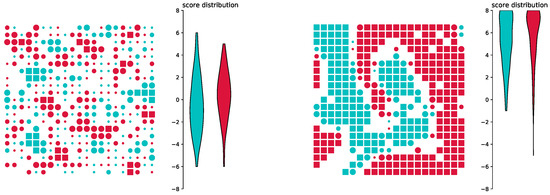
Figure 4.
Reproducing Schelling’s original model: Agents are positioned randomly initially (left), but when using a trained neural network for decision making, they transition into an ordered state (right).
This result cannot be taken for granted, since application of the framework to reproduce a model is more than a simple optimisation. Agents have no knowledge about the way their score is calculated, nor do they know the meaning of the sensory input data and how their actions affect them and their score. All behaviour is learned during the generic experience phase. Nevertheless, it was possible to gain very similar results to the original segregation model, but without the need to define rules, serving as a proof of concept that suggests that also other systems, where it is difficult to find correct rules, can be modelled using the framework.
3.2. Training in a Different Environment
Beyond this proof of concept, we also investigate what happens if we use an environment during application that is different to the one used in training. Here, we use a population consisting of a majority of blue agents and only a few red agents. Results of this simulation can be seen in Figure 5. Figure 5 (left) shows a random configuration during training. Even though the positioning is completely random, blue agents tend to have a higher score, simply because the density of blue agents is much higher. After the training phase, we change the population to a symmetrical population share and use the trained neural network for decision making. In Figure 5 (right), we see the final configuration after 100 time steps. It is clearly visible that red and blue agents learned completely different behaviour. Blue agents are only satisfied with very high scores and cluster together very closely. Red agents learned that high scores are difficult to obtain and are thus satisfied with a lower score, even though higher scores would be obtainable in this system. We also see blue agents that are encircled by red agents. The reason for this behaviour is that the blue agents never encountered such a situation during training and are not sure what to do, leading to a wrong decision.
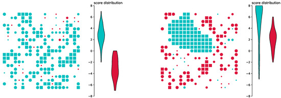
Figure 5.
Different environment for training and application: If agents are trained in an environment with an asymmetric population share, the different groups of agents learn different behaviour. Even if the groups are the same size during application, the group that was under-represented during learning is satisfied with a lower score.
3.3. Truncating Input during Training
Models where the agents are not capable of perfectly classifying all actions are especially interesting for the presented framework. Such a situation can be achieved by truncating the senses of the agents during training, representing a system with a suboptimal learning environment. Figure 6 shows the results of such a simulation run. Even with all their senses enabled during application, they tend to ignore input that they cannot relate to a previous experience. Figure 6 (left) shows the final configuration of a simulation, where agents were only able to see their left and their right neighbour, but nothing else. This leads to the agents forming horizontal lines. In Figure 6 (right), red agents could only sense left and right, blue agents could only sense up and down during training. The result is the formation of horizontal lines for the red agents and vertical lines for the blue agents. Overall score is higher than for Figure 6 (left), since the different orientation aids pattern formation.
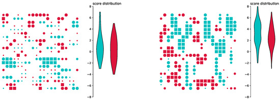
Figure 6.
Truncating the senses during training: If agents can only see in certain directions during training, the resulting patterns during application differ, even if during this phase the agents see all their neighbours.
4. Discussion
The obtained results show that it is possible to use the framework to generate a model that produces very similar results to Schelling’s original model. The most striking difference is that trained agents do not make a perfect decisions all the time. Sometimes they perform actions that decrease their scores, which would not happen if they would correctly classify all actions available to them. This is possible because the neural network is not trained until it has 100% accuracy in solving any classification problem, but under realistic conditions to produce realistic behaviour. This inaccuracy goes beyond the typical problem of generalisation in neural networks: Part of the information that would be needed for correct classification is simply not available to the agents. In the presented example, the average density of agents of a certain colour would be crucial to determine if moving away from a spot would most likely increase or decrease the current score, yet this density is not perceived by the agents and therefore has no influence on their decision.
To highlight the difference between a perfect decision (i.e., correct classifications throughout, as would be the goal of reinforcement learning) and a realistic decision, we truncate the sensory input that agents receive. As expected, agents are then unable to correctly judge many of the possible situations and behave differently. Again, the model provides realistic results without the need to manually define agent behaviour.
While the model was able to successfully reproduce Schelling’s segregation model, there are also several possible ways to expand it in order to increase its scope. Currently, the agents only consider the direct effects of their action. This is sufficient for the used model, but other models would require the agents to think ahead several steps in order to behave realistically. To solve this problem, the model would need a small adaptation. Instead of judging the effect of their next action, they need to judge the effect of their next few actions. If the number of available actions or the number of steps becomes to large to evaluate all possible options, a Monte-Carlo approach using a Markov process [45,46] may be used, or even more sophisticated techniques from reinforcement learning, such as efficient exploration [47,48,49]. These techniques are able to filter out the most promising options and evaluate them carefully, while ignoring options that have a low chance of success, thus drastically reducing the sample space that needs to be considered in order to make a decision.
Another difficulty that one could encounter when applying the framework to different systems is related to the experience phase. For the presented application, random decisions were sufficient to generate a satisfying training environment. However, this is not true for all systems. In many systems, the environment produced by realistic decisions is fundamentally different from the environment produced by random decisions, thus making it unsuitable for training the agents. In that case, it might be better to train the agents iteratively. After the first training, agents could enter a second experience phase in which they collect data in the same way as previously, but with decisions utilising the neural network instead of random decisions. This process could be repeated until convergence. However, since generating smart decisions is computationally more expensive than generating random decisions, such a process would drastically increase the time required for training.
Using the framework offers unique benefits. While rules are hard to define and even harder to justify, finding a way of scoring the success of an agent is straightforward most of the time, as is apparent for the example of modelling a game of chess. In addition, finding an appropriate training environment for the agents is easier than finding rules, mainly because such an environment is more visible in the real world than some underlying rules. Furthermore, in many cases, the training environment is completely identical to the application environment. However, using a different training environment offers new flexibility and ways of influencing agent behaviour, as was demonstrated by changing the agent density during the training phase. As long as the training environment is realistic, the resulting agent behaviour is also realistic. On the other hand, an unrealistic training environment will lead to unrealistic behaviour. Since an unrealistic training environment is easier to spot and identify than an unrealistic rule set, using the framework also reduces the risk of errors in model development, to which agent-based models are usually very susceptible [50,51,52].
Further steps in the development of the framework will be its application to many different systems where established models are available for comparison, in order to gain insight into its flexibility and improve it where necessary. After this step, application can be expanded to systems where there is as of yet no satisfying agent-based solution. Possible areas for such tests would be cooperation research [11,53,54], game theory [55,56,57] or sociology [58,59,60,61].
After the framework is sufficiently tested, so that we can ensure that it can be used for most systems suitable for agent-based modelling, it will be made available as open-source software, so that it can be used and modified by the whole research community and beyond. This would facilitate the diffusion of agent-based modelling and provide easy access to this methodology. The current implementation of the framework and the presented model is done in Python, thus all data are transferred directly. Future plans include a flexible interface, so that models programmed in a different language (e.g., NetLogo) can also benefit from the framework.
5. Conclusions
We identified the search for rules that govern the agent behaviour as the most challenging step in the development of agent-based models. Since the decision process for agents in most systems consists of picking the best alternative, given a finite set of choices, we propose to use a trained neural network to handle this decision as a classification problem. We introduced a generic framework, in which we do not need to define rules, but a score and a training environment for the agents. As a poof of principle, we use the framework to reproduce Schelling’s segregation model. We found that, even without specifying rules, we can develop a model that produces the same results as Schelling’s original segregation model, but with the added possibility to change the training environment, giving us more flexibility. Thus, this study substantiates the claim that it is possible to derive a generic framework for agent-based models using artificial neural networks. Nevertheless, more work needs to be done before the framework can be applied to an arbitrary system, which would be the final goal of developing this framework.
Funding
This research received no external funding.
Acknowledgments
Open Access Funding by the University of Graz.
Conflicts of Interest
The author declares no conflict of interest.
References
- Gilbert, N. Agent-Based Models; Number 153; Sage: Thousand Oaks, CA, USA, 2008. [Google Scholar]
- Chen, X.; Zhan, F.B. Agent-based modelling and simulation of urban evacuation: Relative effectiveness of simultaneous and staged evacuation strategies. J. Oper. Res. Soc. 2008, 59, 25–33. [Google Scholar] [CrossRef]
- Chen, B.; Cheng, H.H. A review of the applications of agent technology in traffic and transportation systems. IEEE Trans. Intell. Transp. Syst. 2010, 11, 485–497. [Google Scholar] [CrossRef]
- Balmer, M.; Cetin, N.; Nagel, K.; Raney, B. Towards truly agent-based traffic and mobility simulations. In Proceedings of the Third International Joint Conference on Autonomous Agents and Multiagent Systems-Volume 1; IEEE Computer Society: Washington, DC, USA, 2004; pp. 60–67. [Google Scholar]
- Hofer, C.; Jäger, G.; Füllsack, M. Large scale simulation of CO2 emissions caused by urban car traffic: An agent-based network approach. J. Clean. Prod. 2018, 183, 1–10. [Google Scholar] [CrossRef]
- Batty, M. Cities and Complexity: Understanding Cities With Cellular Automata, Agent-Based Models, and Fractals; The MIT press: Cambridge, MA, USA, 2007. [Google Scholar]
- Davidsson, P. Agent based social simulation: A computer science view. J. Artif. Soc. Soc. Simul. 2002, 5, 1–7. [Google Scholar]
- Epstein, J.M. Agent-based computational models and generative social science. Complexity 1999, 4, 41–60. [Google Scholar] [CrossRef]
- Bonabeau, E. Agent-based modeling: Methods and techniques for simulating human systems. Proc. Natl. Acad. Sci. USA 2002, 99, 7280–7287. [Google Scholar] [CrossRef]
- Judson, O.P. The rise of the individual-based model in ecology. Trends Ecol. Evol. 1994, 9, 9–14. [Google Scholar] [CrossRef]
- Axelrod, R.M. The Complexity of Cooperation: Agent-Based Models of Competition and Collaboration; Princeton University Press: Princeton, NJ, USA, 1997. [Google Scholar]
- Amman, H.M.; Tesfatsion, L.; Kendrick, D.A.; Judd, K.L.; Rust, J. Handbook of Computational Economics; Elsevier: Amsterdam, The Netherlands, 1996; Volume 2. [Google Scholar]
- Tesfatsion, L. Agent-based computational economics: Growing economies from the bottom up. Artif. Life 2002, 8, 55–82. [Google Scholar] [CrossRef]
- Tesfatsion, L. Agent-based computational economics: A constructive approach to economic theory. Handb. Comput. Econ. 2006, 2, 831–880. [Google Scholar]
- Deissenberg, C.; Van Der Hoog, S.; Dawid, H. EURACE: A massively parallel agent-based model of the European economy. Appl. Math. Comput. 2008, 204, 541–552. [Google Scholar] [CrossRef]
- Farmer, J.D.; Foley, D. The economy needs agent-based modelling. Nature 2009, 460, 685–686. [Google Scholar] [CrossRef] [PubMed]
- Gilbert, G.; Hamill, L. Social circles: A simple structure for agent-based social network models. J. Artif. Soc. Soc. Simul. 2009, 12, 1–3. [Google Scholar]
- Andrei, A.L.; Comer, K.; Koehler, M. An agent-based model of network effects on tax compliance and evasion. J. Econ. Psychol. 2014, 40, 119–133. [Google Scholar] [CrossRef]
- Simon, H.A. Theories of bounded rationality. Decis. Organ. 1972, 1, 161–176. [Google Scholar]
- Gilbert, N.; Terna, P. How to build and use agent-based models in social science. Mind Soc. 2000, 1, 57–72. [Google Scholar] [CrossRef]
- Sutton, R.S.; Barto, A.G. Introduction to Reinforcement Learning; MIT Press: Cambridge, MA, USA, 1998; Volume 2. [Google Scholar]
- Kaelbling, L.P.; Littman, M.L.; Moore, A.W. Reinforcement learning: A survey. J. Artif. Intell. Res. 1996, 4, 237–285. [Google Scholar] [CrossRef]
- Schelling, T.C. Models of segregation. Am. Econ. Rev. 1969, 59, 488–493. [Google Scholar]
- Schelling, T.C. Dynamic models of segregation. J. Math. Sociol. 1971, 1, 143–186. [Google Scholar] [CrossRef]
- Yao, X. Evolving artificial neural networks. Proc. IEEE 1999, 87, 1423–1447. [Google Scholar]
- Schmidhuber, J. Deep learning in neural networks: An overview. Neural Netw. 2015, 61, 85–117. [Google Scholar] [CrossRef]
- Silver, D.; Huang, A.; Maddison, C.J.; Guez, A.; Sifre, L.; Van Den Driessche, G.; Schrittwieser, J.; Antonoglou, I.; Panneershelvam, V.; Lanctot, M.; et al. Mastering the game of Go with deep neural networks and tree search. Nature 2016, 529, 484. [Google Scholar] [CrossRef]
- Da Silva, I.N.; Spatti, D.H.; Flauzino, R.A.; Liboni, L.H.B.; dos Reis Alves, S.F. Artificial Neural Networks; Springer International Publishing: Cham, Switzerland, 2017. [Google Scholar]
- Sutskever, I.; Vinyals, O.; Le, Q.V. Sequence to sequence learning with neural networks. In Advances in Neural Information Processing Systems; 2014; pp. 3104–3112. Available online: https://papers.nips.cc/paper/5346-sequence-to-sequence-learning-with-neural-networks.pdf (accessed on 9 October 2019).
- Günther, F.; Fritsch, S. neuralnet: Training of neural networks. R J. 2010, 2, 30–38. [Google Scholar] [CrossRef]
- Zhang, L.; Suganthan, P.N. A survey of randomized algorithms for training neural networks. Inf. Sci. 2016, 364, 146–155. [Google Scholar] [CrossRef]
- Sutskever, I.; Hinton, G. Training Recurrent Neural Networks; University of Toronto: Toronto, ON, Canada, 2013. [Google Scholar]
- Courbariaux, M.; Bengio, Y.; David, J.P. Training deep neural networks with low precision multiplications. arXiv 2014, arXiv:1412.7024. [Google Scholar]
- Mirjalili, S.; Hashim, S.Z.M.; Sardroudi, H.M. Training feedforward neural networks using hybrid particle swarm optimization and gravitational search algorithm. Appl. Math. Comput. 2012, 218, 11125–11137. [Google Scholar] [CrossRef]
- Srivastava, R.K.; Greff, K.; Schmidhuber, J. Training very deep networks. In Advances in Neural Information Processing Systems; MIT Press: Cambridge, MA, USA, 2015; pp. 2377–2385. [Google Scholar]
- Blank, T.; Brown, S. Data processing using neural networks. Anal. Chim. Acta 1993, 277, 273–287. [Google Scholar] [CrossRef]
- Huang, G.B.; Saratchandran, P.; Sundararajan, N. A generalized growing and pruning RBF (GGAP-RBF) neural network for function approximation. IEEE Trans. Neural Netw. 2005, 16, 57–67. [Google Scholar] [CrossRef] [PubMed]
- Adya, M.; Collopy, F. How effective are neural networks at forecasting and prediction? A review and evaluation. J. Forecast. 1998, 17, 481–495. [Google Scholar] [CrossRef]
- Dreiseitl, S.; Ohno-Machado, L. Logistic regression and artificial neural network classification models: A methodology review. J. Biomed. Inform. 2002, 35, 352–359. [Google Scholar] [CrossRef]
- Gauvin, L.; Vannimenus, J.; Nadal, J.P. Phase diagram of a Schelling segregation model. Eur. Phys. J. B 2009, 70, 293–304. [Google Scholar] [CrossRef]
- Clark, W.A.; Fossett, M. Understanding the social context of the Schelling segregation model. Proc. Natl. Acad. Sci. USA 2008, 105, 4109–4114. [Google Scholar] [CrossRef] [PubMed]
- Weisstein, E.W. Moore Neighborhood. From MathWorld—A Wolfram Web Resource. 2005. Available online: http://mathworld.wolfram.com/MooreNeighborhood.html (accessed on 9 September 2019).
- Guyon, I.; Gunn, S.; Nikravesh, M.; Zadeh, L.A. Feature Extraction: Foundations and Applications; Springer: Berlin/Heidelberg, Germany, 2008; Volume 207. [Google Scholar]
- Helbing, D. Agent-based modeling. In Social Self-Organization; Springer: Berlin/Heidelberg, Germany, 2012; pp. 25–70. [Google Scholar]
- Thrun, S. Monte carlo pomdps. In Advances in Neural Information Processing Systems; MIT Press: Cambridge, MA, USA, 2000; pp. 1064–1070. [Google Scholar]
- Lazaric, A.; Restelli, M.; Bonarini, A. Reinforcement learning in continuous action spaces through sequential monte carlo methods. In Advances in Neural Information Processing Systems; MIT Press: Cambridge, MA, USA, 2008; pp. 833–840. [Google Scholar]
- Thrun, S. Efficient Exploration in Reinforcement Learning; Technical Report; Carnegie Mellon University: Pittsburgh, PA, USA, 1992. [Google Scholar]
- Mnih, V.; Kavukcuoglu, K.; Silver, D.; Rusu, A.A.; Veness, J.; Bellemare, M.G.; Graves, A.; Riedmiller, M.; Fidjeland, A.K.; Ostrovski, G.; et al. Human-level control through deep reinforcement learning. Nature 2015, 518, 529. [Google Scholar] [CrossRef] [PubMed]
- Stanley, K.O.; Miikkulainen, R. Efficient reinforcement learning through evolving neural network topologies. In Proceedings of the 4th Annual Conference on Genetic and Evolutionary Computation, New York, NY, USA, 9–13 July 2002; Morgan Kaufmann Publishers Inc.: Burlington, MA, USA, 2002; pp. 569–577. [Google Scholar]
- Jennings, N.R. Agent-Based Computing: Promise and Perils. In Proceedings of the Sixteenth International Joint Conference on Artificial Intelligence, Stockholm, Sweden, 31 July–6 August 1999; Morgan Kaufmann Publishers Inc.: Burlington, MA, USA, 1999; pp. 1429–1436. [Google Scholar]
- Galán, J.M.; Izquierdo, L.R.; Izquierdo, S.S.; Santos, J.I.; Del Olmo, R.; López-Paredes, A.; Edmonds, B. Errors and artefacts in agent-based modelling. J. Artif. Soc. Soc. Simul. 2009, 12, 1. [Google Scholar]
- Leombruni, R.; Richiardi, M. Why are economists sceptical about agent-based simulations? Phys. A Stat. Mech. Its Appl. 2005, 355, 103–109. [Google Scholar] [CrossRef]
- Elliott, E.; Kiel, L.D. Exploring cooperation and competition using agent-based modeling. Proc. Natl. Acad. Sci. USA 2002, 99, 7193–7194. [Google Scholar] [CrossRef] [PubMed]
- Müller, J.P. A cooperation model for autonomous agents. In Proceedings of the International Workshop on Agent Theories, Architectures, and Languages; Springer: Berlin/Heidelberg, Germany, 1996; pp. 245–260. [Google Scholar]
- Parsons, S.D.; Gymtrasiewicz, P.; Wooldridge, M. Game Theory and Decision Theory in Agent-Based Systems; Springer Science & Business Media: Berlin/Heidelberg, Germany, 2012; Volume 5. [Google Scholar]
- Adami, C.; Schossau, J.; Hintze, A. Evolutionary game theory using agent-based methods. Phys. Life Rev. 2016, 19, 1–26. [Google Scholar] [CrossRef] [PubMed]
- Semsar-Kazerooni, E.; Khorasani, K. Multi-agent team cooperation: A game theory approach. Automatica 2009, 45, 2205–2213. [Google Scholar] [CrossRef]
- Conte, R.; Edmonds, B.; Moss, S.; Sawyer, R.K. Sociology and social theory in agent based social simulation: A symposium. Comput. Math. Organ. Theory 2001, 7, 183–205. [Google Scholar] [CrossRef]
- Bianchi, F.; Squazzoni, F. Agent-based models in sociology. Wiley Interdiscip. Rev. Comput. Stat. 2015, 7, 284–306. [Google Scholar] [CrossRef]
- Macy, M.W.; Willer, R. From factors to actors: Computational sociology and agent-based modeling. Annu. Rev. Sociol. 2002, 28, 143–166. [Google Scholar] [CrossRef]
- Squazzoni, F. Agent-Based Computational Sociology; John Wiley & Sons: Hoboken, NJ, USA, 2012. [Google Scholar]
© 2019 by the author. Licensee MDPI, Basel, Switzerland. This article is an open access article distributed under the terms and conditions of the Creative Commons Attribution (CC BY) license (http://creativecommons.org/licenses/by/4.0/).