1. Introduction
Salient object detection has attracted a lot of interest in the computer vision community. It allows us to quickly retrieve information from the input image by focusing on the most conspicuous object regions [
1]. The fundamental challenge of salient object detection is to find the decision boundary that separates the salient object from the background.
Many saliency detection methods have been proposed to address this challenge. Depending on whether large scale training samples are used or not, existing methods broadly fall into two categories: Supervised and unsupervised. In many situations, data-driven supervised methods can provide a workable solution strategy and produce a clean saliency map. Liu et al. [
2] proposed to detect salient object by formulating the detection process as a binary labeling problem. They first extracted multiple levels (locally, regionally, and globally) image features. Following this, the features were used to train a conditional random field (CRF) for detecting the saliency map. Mai et al. [
3] proposed to use a data-driven based CRF approach to perform saliency aggregation in order to mitigate the performance gaps among other salient object detection methods. Jiang et al. [
4] formulated the saliency detection task as a regression problem via the random forest model. First, they divided the image into multi-level regions to form multi-level image segmentation. Then each region was represented by discriminative features. Later, the features were used to train a random forest regressor to map them to saliency values. Finally, saliency values from different regions and levels were linearly combined to achieve the final saliency map. Recently, the successful applications of deep neural networks (DNNs) in various research fields open up another promising path for accurately detecting salient objects. In [
5], a multi-context deep learning method for saliency detection is proposed. The work first employed a global-context convolutional neural network (CNN) to acquire the image-level information. It then created a local-context modeling CNN to get closer-focused local information, by inputting image patches. The results of the two networks were combined to obtain the final saliency map. Li et al. [
6] proposed to use a pixel-level fully CNN stream to obtain the pixel-level saliency prediction result. At the same time, they used a segment-wise spatial pooling stream to extract the segment-wise feature. Finally, they used a CRF to incorporate the results of the two streams to generate the final saliency map. Hou et al. [
7] proposed a short-connection deep supervised salient object detection method. They connected the output from the other side output of hidden layers to the last pooling layer in CNN to enhance the visual distinctive region output. These data-driven supervised methods achieved remarkable detection performance in detecting the task-specified salient object. However, the detection accuracy of these supervised methods was restricted by the quality and quantity of training samples and the high computational platform required for deep learning-based methods.
On the other hand, many sophisticated approaches have been proposed to deal with the salient object detection task in an unsupervised or weakly-supervised manner. Most of them attempted to identify saliency regions in a scene via low-level features, such as color, texture, and location. Among the unsupervised saliency detection methods, the most commonly used methods are contrast-based methods [
8,
9] and mathematical model-based methods [
10,
11,
12,
13]. As one of the contrast-based saliency detection methods, the work in [
9] proposed a contrast-filtering method. First, they split the input image into basic elements that preserve the relevant image structure. After this, they calculated two contrast metrics based on the uniqueness and spatial distribution of the elements in order to find the significance value of each element. Finally, they used high-dimensional Gaussian filters to estimate the saliency map. In [
8], Cheng et al. proposed a regional contrast saliency detection method. This method used the histogram-based contrast to calculate the global color information. Then, a region-based contrast was proposed to enhance the spatial information on the final saliency map. Ishikura et al. [
14] proposed an unsupervised saliency detection method based on multi-scale extrema of local perceptual color difference. However, their method was only used to estimate the locations, sizes, and saliency levels of candidate regions instead of the pixel-level saliency map.
Research has also been conducted on saliency detection methods based on mathematical models. Wang et al. [
11] adopted the site entropy rate model. First, the multi-band filter response maps were calculated, and then the response map was represented by a fully-connected graph based on cortical connectivity. The site entropy rate (SER) was used to measure the average information from a node to the others in the graph. The final saliency map was calculated by using the cumulative sum of all SERs. Later, Guo et al. [
12] proposed a SER based multi-scale point set saliency detection method. The most representative mathematical model for saliency detection is the low-rank matrix recovery (LRMR)-based (or low-rank and sparse matrix decomposition) model. In the LRMR model, the saliency detection task is formulated as the decomposition of a feature matrix. The model decomposes the feature matrix into a sparse subspace and a low-rank subspace [
10]. It assumes that the low-rank feature space represents the redundant background image information and the salient object is represented in the sparse feature space. These unsupervised methods have the generalized ability for unseen saliency detection tasks.
The LRMR based saliency detection method is simple and powerful. However, the detection performance is usually restricted by spatial consistency and incomplete detection results. It is because LRMR loses spatial consistency during the mathematical analysis process of converting three-dimensional (3D) image feature into two-dimensional (2D) matrix, while not taking full advantage of image features. In this article, our main interest is in seeking to maintain the spatial consistency to improve the detection accuracy. With the aid of high-dimensional tensor decomposition, we are able to solve this issue and derive better salient object detection results.
The main contribution of this article is twofold: (1) to the best of our knowledge, this is the first attempt to integrate tensor decomposition into the salient object detection task. By doing this, we can naturally represent high-dimensional features with a tensor. We then propose a series relaxation optimization processes to simplify the optimization process of tensor decomposition and solve it by using a heuristic method; (2) tensor decomposition is capable of discovering more hidden relationships of image features than LRMR in the process of capturing saliency information. Therefore, it obtains better salient object detection accuracy as shown in the experimental results section.
2. Related Works
In this section, we briefly review the work of LRMR-based salient object detection and basic knowledge about tensors.
The core of LRMR is decomposing a 2D matrix space into a sparse subspace and a low-rank subspace. Mathematically, LRMR can be formulated as [
15]:
where
represents the input 2D image or the feature matrix. As shown in Equation (1),
F is decomposed into the sum of a low-rank matrix
and sparse matrix
by solving optimization problem in Equation (1).
stands for the nuclear norm which computes the sum of the singular values of a matrix. It is a convex relaxation of the matrix rank function.
represents the
l1-norm to promote the sparsity.
λ is a constant to balance the tradeoff between the low-rank term and the sparse term.
In the literature on salient object detection via LRMR, the work by Yan et al. [
16] was the earliest attempt. They suggested segmenting the input image into small patches. From these image patches, they learned an over-completed dictionary. Then, the sparse coding features obtained from the learned dictionary constituted the feature space of the input image. The LRMR was performed in this feature space to generate the sparse matrix, and then it was used to produce the final saliency map. Peng et al. [
1] pointed out that most LRMR-based methods did not take into consideration the inter-correlation between salient elements. Therefore, they proposed a
structured matrix decomposition (SMD) model for saliency detection. The SMD model leverages a tree-structure during the LRMR decomposition process to smooth the detected saliency region and capture spatial relations between salient elements. However, Zheng et al. [
17] mentioned that the deep structure of the tree in SMD may destroy the sparsity of LRMR decomposition. They proposed to maintain the completeness of the salient object through a coarse-to-fine integration process. Moreover, the work in [
18] aimed to improve the salient performance by adding global prior as the weight of LRMR during matrix decomposition process. In summary, the salient object detection methods refer to LRMR focusing on one key objective: Properly modeling image features to separate the low-rank background from the sparse salient objects, while sustaining the completeness of the salient object. In this article, we propose to use the low-rank and sparse tensor method to achieve this objective.
A tensor is a multidimensional array [
19,
20]. We used bold capital fonts to represent the matrix, while a boldface script letter, e.g.,
, was used to denote a tensor. A vector is a first-order tensor, and a matrix is a second-order tensor. Here, the order of a tensor is the number of dimensions. Similar to matrix rows and columns, a third-order tensor has column, row, and tube fibers. A tensor can reorder its elements to form a matrix, i.e., unfolding. The mode-
n unfolding of a tensor
is denoted by
and arranges the mode-
n fibers to be the columns of the resulting matrix [
19]. For instance, a 3 × 4 × 5 tensor can be arranged as a 3 × 20 matrix, or a 4 × 15 matrix, or a 5 × 12 matrix. For a more complete knowledge of tensor and tensor decomposition, please refer to [
19,
20]. Due to high-dimensional data representation and analysis capabilities, tensor and tensor decomposition have been widely adopted in various research fields. For example, Jia et al. [
21] proposed to use low-rank tensor decomposition for recognizing RGB-D action. They used the tensor Tucker decomposition to obtained tensor ranks. The obtained tensor ranks can be used to discover tensor subspace to extract useful information of RGB-D action. The work in [
22] emphasized tensor-based decomposition techniques for detecting abnormalities and failures in different applications, such as environmental monitoring, video surveillance, social networks, etc. In these applications, different spatial and time series data are represented by tensor, and different techniques, such as tensor classifiers, tensor forecasting, and tensor decomposition, to consider the mutual relationship between different dimensions in the tensor. Chen and Mitra [
23] proposed to use tensor Tucker decomposition-based technique to locate the source from multimodal data. Specifically, they used rank-1 tensor resulted from Tucker decomposition to compute the common signature vectors. Then, the peak locations of the signature vectors represent the coordinate of the source location. In this work, we attempted to use tensor solving salient object detection task by leveraging its high-dimensional representation ability.
We extend the matrix based low-rank and sparse decomposition into high-dimensional tensor version and apply it to the salient object detection task. The motivations for our work are: First, the high-dimensional tensor is able to express image features in their natural way. As a result, the spatial information of the image is well maintained. Second, the proposed low-rank and sparse tensor decomposition discovers useful information from high-dimensional feature analysis. Therefore, it achieves better performance in discovering salient objects than its LRMR based counterpart methods.
3. Proposed Tensor Decomposition Method for Saliency Detection
For image detection tasks, a rich image feature space is often required to capture high object variations to improve detection performance. In order to adapt LRMR to the salient object detection task, existing methods convert high dimensional feature space into 2D to accomplish model fitting process, while at the expense of spatial consistency. To sustain both the effectiveness of LRMR and the spatial consistency, we propose low-rank and sparse tensor decomposition method.
Based on Equation (1), low-rank and sparse tensor decomposition can be written as:
Accordingly, , , are the input three-dimensional (3D) image or feature tensor, low-rank tensor, and sparse tensor, respectively.
However, unlike matrices, computing the rank of a tensor with the order greater than two is a non-deterministic polynomial-time (NP) hard problem, because the definition of tensor rank depends on the choice of the field [
24]. Therefore, most works used heuristic-based strategies, such as in [
21,
23]. In this work, to solve Equation (2), we also employ a heuristic-based method by redefining the trace norm and
l1-norm for the high-dimensional tensor case with the order greater than three. Based on the relationship between high-dimensional tensor and matrix, we use the following tensor trace norm [
25] for a
n-order tensor
:
To simplify the computation here in this article and to be consistent with the above trace norm, we propose the following tensor
l1-norm:
where
’s and
’s are constants satisfying
and
. In essence, the trace norm (or
l1-norm) of a high-dimensional tensor is a linear combination of the trace norms (or
l1-norms) of all matrices unfolded along each mode. Note that, the
l1-norm definition in this article is different from the general norm definition of a tensor in [
19].
Therefore, with these definitions, the optimization in Equation (2) can be written as:
Equation (5) with known tensor
aims at finding the minimal summation value of n linear equations. To solve this, we replace it with
n-sub-problem and find minimal values of each sub-problem, and then we summarize
n-minimal values together to achieve the final result of Equation (5), with the aid of tensor unfolding.
To solve the non-convex sub-problem of Equation (6), the robust principal component analysis (RPCA) method [
26] can be properly employed. That is, we unfolding the obtained image feature tensor
into three matrices,
,
,
, after optimization using the RPCA method, we obtain three matrices
of the tensor
. Therefore, our tensor decomposition turns into three LRMR optimization problems:
In this article, this heuristic method is called tensor decomposition original (TDO). In this case, the basic LRMR model becomes the second sub-problem of our case. LRMR is the second unfolding situation of our tensor decomposition. After we obtain three sparse matrices , we summarize them according to weights to obtain final saliency tensor . Finally, the l1-norm along each tube fibers, i.e., , of tensor is used to measure the saliency of corresponding segmented region in the i-th row and j-th column of the superpixels. The final saliency map is then accordingly generated and normalized to a 0 to 1 scale image.
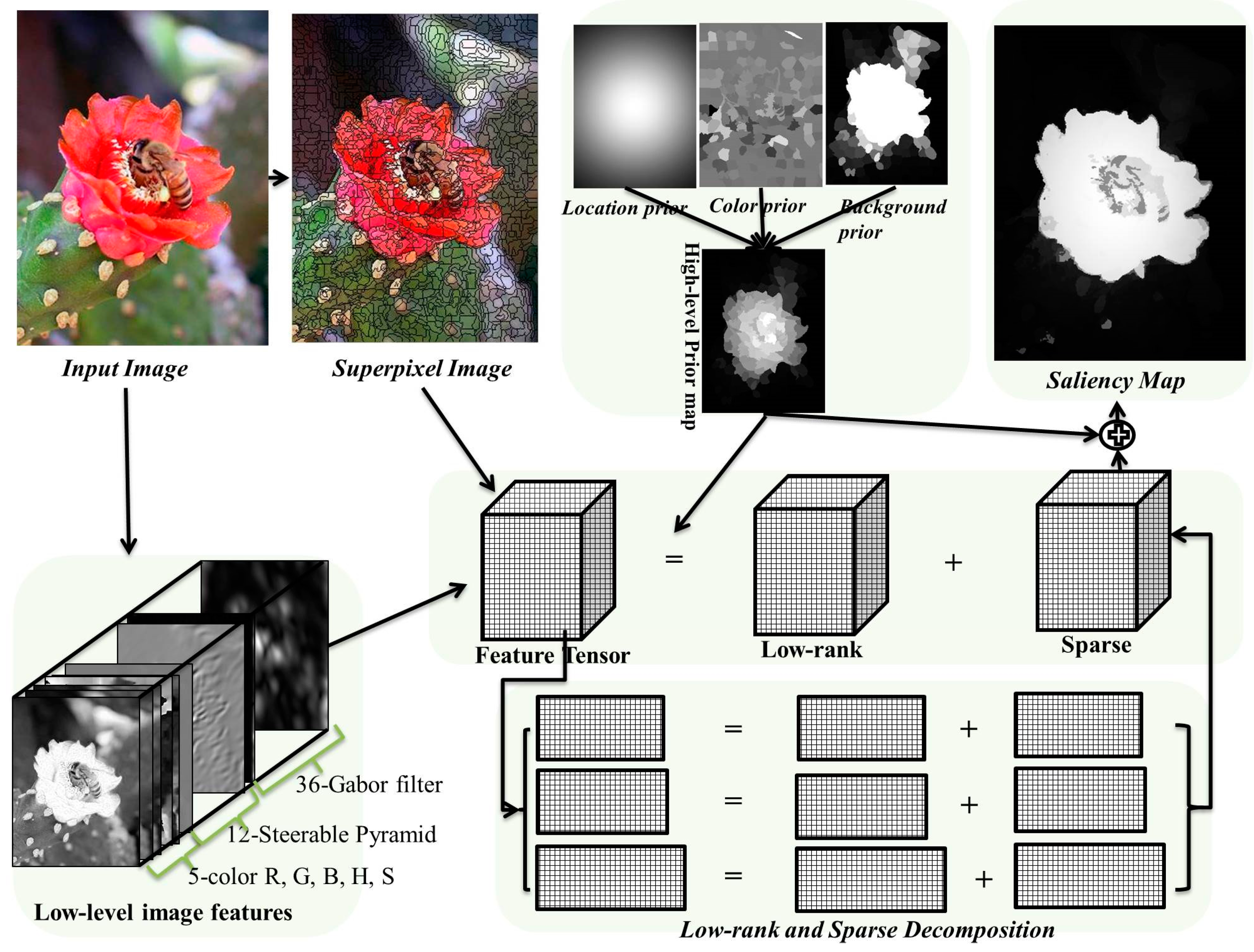
Following this we can then adapt Equation (5) to a salient object detection task. The overview of our framework is shown in
Figure 1. Given an input image
, its low-level features including color, steerable pyramids [
27], and Gabor filter [
28], are calculated, forming a
P × Q × D feature tensor (in this article
D = 53). The Gabor filter feature captures the edge, texture information of the input image. These low-level features can better represent the input image than raw pixel values. Note, here we use the same low-level features as in [
1] for a fair comparison in
Section 4. The feature tensor is segmented into
M × N small non-overlapping regions, i.e., superpixels, using the
simple linear iterative clustering (SLIC) method [
29] to reduce the computational cost. Each small region is assigned with a
D-dimensional feature vector which equals to the mean feature values over all the pixels within the region. Finally, all regions, together with their feature vectors, constitute the input tensor
. Then we use Equation (6) based heuristic procedures to solve this image feature-based tensor decomposition.
Similar to [
1], we also integrated high-level priors into our tensor decomposition process, in order to guide the decomposition slightly incline to the most empirically potential saliency position of an image. Three types of priors including location, color, and background priors are used to generate a high-level prior weight map. Empirically, the probability of a salient object in the center of the image is higher than the boundary of the image. The location prior models this observation through a Gaussian distribution based on the distances of the pixels from the image center. Since the human eye is sensitive to red and yellow color, the color prior [
10] tends to pay more attention to these color regions in an image. The background prior [
30] treats image boundaries as background with high probability. In addition, the high-level prior is employed to eliminate noise saliency regions for the final saliency map.
5. Discussion
In this section, we discuss the results shown in
Section 4 from the perspectives of our research motivations and future work.
In this article, we proposed a tensor decomposition method to detect the salient object from images. The task was formulated as a tensor low-rank and sparse optimization problem. We employed a heuristic method to convert the optimization problem into three sub-problems.
• The first motivation of this article is that we use a tensor to represent image features in a natural high-dimensional fashion. The tensor ensures that more dimensions can be introduced to represent information; meaning that the spatial information is maintained.
One of the drawbacks of LRMR based methods in saliency detection is that it may destroy the spatial consistency when converting high-dimensional image features into 2D matrix form. It is because the spatial adjacent image regions are separated in the feature space. The SMD method addressed this drawback by introducing a tree-structure to group spatial adjacent image regions together during the optimization process. However, in this article, we used a tensor to represent the image feature to maintain the spatial position of image regions. Although the heuristic optimization may change this 3D structure during the individual optimization process, the final step of converting the result of the optimized sub-problems into a single tensor will solve the spatial connection problem.
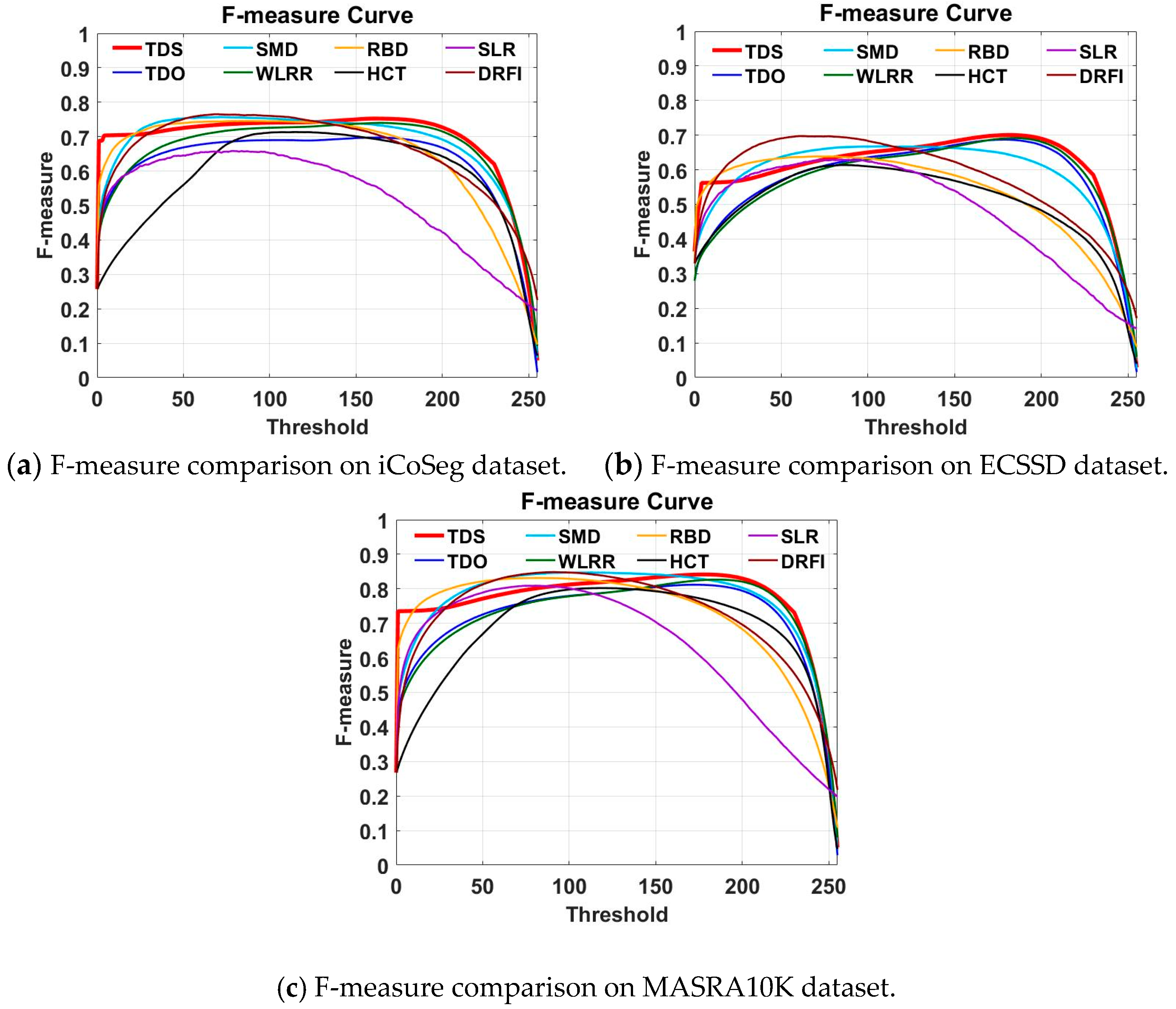
As can be observed from
Table 1,
Table 2 and
Table 3 and
Figure 3, the original tensor decomposition method TDO achieved a much higher performance than the LRMR-method SLR, which did not consider spatial information. However, it achieved a slightly worse performance than SMD and WLRR with their additional tree-structure and weighted prior information, respectively. The reason for this is that TDO contains more noise information during the tensor decomposition process. Therefore, we used the high-level prior information to generate a mask to reduce the saliency value in high probability background area to obtain the final saliency map, i.e., TDS. As a result, the MAE was reduced in TDS. TDS achieved slightly higher or similar performance than SMD and WLRR in terms of the metrics. This means the proposed tensor method has the ability to sustain the spatial structure.
• The second motivation for this study is that tensor decomposition is capable of discovering more saliency information.
The image feature information was identical for the LRMR-based method and TDS for the salient object detection task. The only difference was the way of representing the image feature. With TDS, the image feature was represented in 3D tensor. Our task was to employ a heuristic method to solve a tensor decomposition problem. This heuristic method converted the tensor into sub-matrices and optimized them independently. Following this, the final tensor decomposition result was obtained by combining three matrices into a unified tensor. Conventional LRMR was just one of our sup-optimization processes.
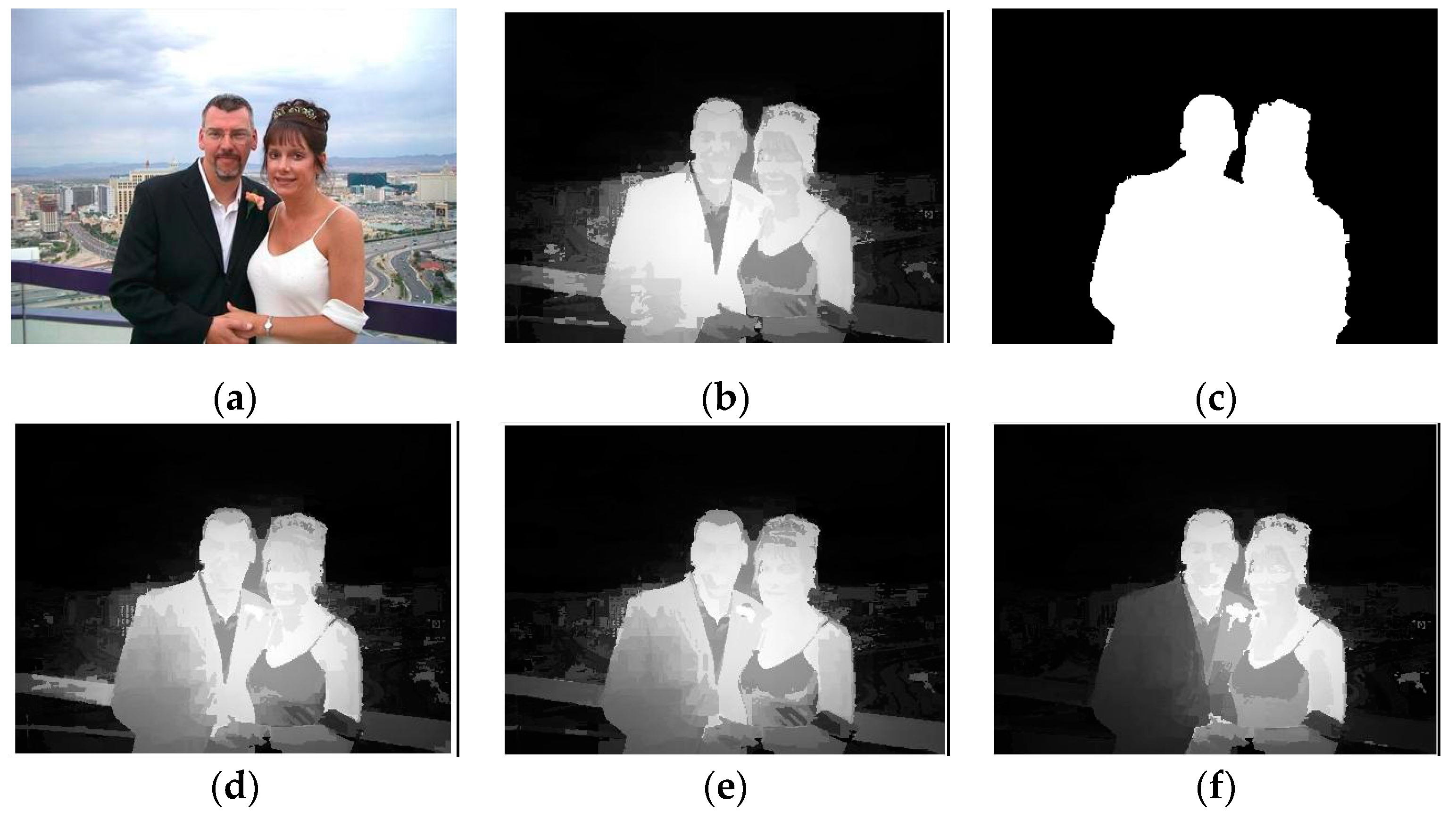
As shown in
Figure 2, each of the three sub-problems extracted saliency regions of the image (
Figure 2d–f). The tensor, which is obtained by integrating the three results from sub-problems, yielded the best saliency map (
Figure 2b). Therefore, the sub-problems complement each other.
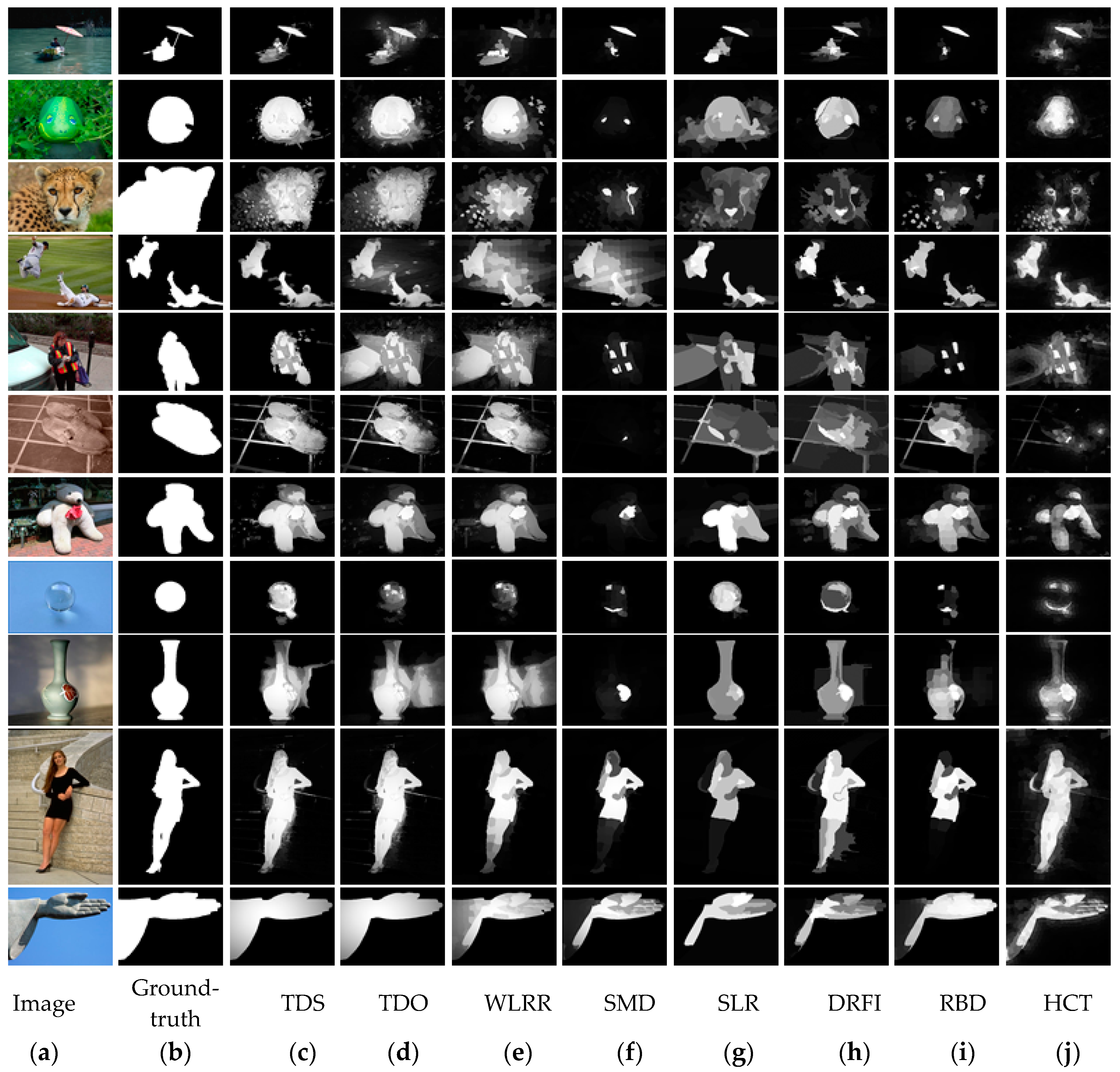
In
Figure 4, we visualize some of the saliency map detected by the proposed method (in columns (c,d) and other methods. It can be observed that, firstly, with the high-prior map, TDS obtained cleaner saliency maps than TDO, as shown in rows 5 and 9. This verifies that TDS achieved better numerical performance than TDO, as shown in
Table 1,
Table 2 and
Table 3. Second, compared to the LRMR-based methods SMD, SLR, TDS, and WLRR, TDS was capable of extracting more salient object information as shown in rows 3, 4, 8, and 11. In addition, saliency maps in column (c) were closer to ground-truth saliency maps in column (b) than other methods like DFI, RBD, and HCT, indicating the effectiveness of the proposed method.
Therefore, we can conclude that tensor decomposition yields more saliency information than LRMR.
• Future work
In this work, we proved that by using a tensor we can sustain spatial information and discover more information related to the saliency area in an image. Therefore, the results are mainly compared with LRMR-based methods. Improving the overall salient detection rate will be the basis of our future work. For example, we can use deep learning-based features, instead of 53-D low-level features in our framework, because deep learning-based features may have better representation ability for salient objects than low-level image features.
In addition, although we propose to use high-dimensional low-rank and sparse tensor decomposition to represent the salient detection task, the tensor decomposition is still converted to the low-rank and sparse matrix decomposition sub-problems during the optimization process. This may affect the optimization result of tensor decomposition. In the future, we will optimize the tensor decomposition from high dimensional aspects, such as using tensor Tucker decomposition, in order to improve the accuracy of the detection result.


