Article

A Data-Driven Machine Learning Approach for Corrosion Risk Assessment—A Comparative Study

School of Information Technology & Mathematical Sciences, University of South Australia, Mawson Lakes Campus, GPO Box 2471 Adelaide, SA 5001, Australia
Big Data Cogn. Comput. 2019, 3(2), 28; https://doi.org/10.3390/bdcc3020028
Submission received: 13 March 2019 / Revised: 8 May 2019 / Accepted: 14 May 2019 / Published: 18 May 2019

Abstract

:
Understanding the corrosion risk of a pipeline is vital for maintaining health, safety and the environment. This study implemented a data-driven machine learning approach that relied on Principal Component Analysis (PCA), Particle Swarm Optimization (PSO), Feed-Forward Artificial Neural Network (FFANN), Gradient Boosting Machine (GBM), Random Forest (RF) and Deep Neural Network (DNN) to estimate the corrosion defect depth growth of aged pipelines. By modifying the hyperparameters of the FFANN algorithm with PSO and using PCA to transform the operating variables of the pipelines, different Machine Learning (ML) models were developed and tested for the X52 grade of pipeline. A comparative analysis of the computational accuracy of the corrosion defect growth was estimated for the PCA transformed and non-transformed parametric values of the training data to know the influence of the PCA transformation on the accuracy of the models. The result of the analysis showed that the ML modelling with PCA transformed data has an accuracy that is 3.52 to 5.32 times better than those carried out without PCA transformation. Again, the PCA transformed GBM model was found to have the best modeling accuracy amongst the tested algorithms; hence, it was used for computing the future corrosion defect depth growth of the pipelines. This helped to compute the corrosion risks using the failure probabilities at different lifecycle phases of the asset. The excerpts from the results of this study indicate that my technique is vital for the prognostic health monitoring of pipelines because it will provide information for maintenance and inspection planning.

1. Introduction

The corrosion of pipelines has caused numerous problems for the operators of oil and gas companies due to the costs associated with the management. These problems have been predominately caused by the operating parameters that are associated with water chemistry, flow attributes, the material properties of the pipeline and microbiological activities [1,2]. Corrosion mitigation is one of the challenges for oil and gas companies because of the complexities of corrosion defect initiation, stabilization and progression. To this end, relevant stakeholders have developed architectures that have the capability of intelligently estimating the corrosion defect growth.
Uniform corrosion of carbon steel material depends on an electrochemical reaction at the steel surface; a fusion process across the porous oxide film surfaces and the migration of the corrosion species [3]. This movement of the corrosive species is caused by the unpredictability of the concentration of the solvents in which the exchange of the cation and anion occur [3]. This in turn results in the build-up of the protective oxide films that temporarily coat the surface of the steel material to prevent more corrosion [4]. However, due to the mechanical actions of the abrasive species and turbulence coming from the fluid flowing in the pipelines, the protective oxides’ coatings are always eroded in a short time, resulting in more corrosion. The work of many researchers in this area has hinged on models that are mainly deterministic, stochastic and empirical using field, simulated and experimental data [4,5,6,7,8,9,10]. Amongst these articles are the time-dependent stochastic models and the characterization of corrosion defect growth by exponential and logarithmic models by authors referenced in [11] and [12]. The researchers determined the reliability of pipelines at different times after exposure to corrosion and computed the corrosion growth rate over time. Other authors [13,14,15] applied the Markov decision process as a continuous-time, non-homogenous linear growth pure birth model and estimated the time-dependent corrosion growth. This method helped the researchers to evaluate corrosion defect depth using multi-regression and power law models, which were also used by other experts in corrosion studies [11,12].
Notwithstanding the gains made in corrosion evaluation via systematic modelling of the defect growth with time, there are still numerous questions that are yet to be answered on corrosion defect growth estimation. To this end, many experts are still not conclusive on the trends and the expected timing of corrosion defect growth. As a result of these doubts, other scholars have veered toward artificial intelligence as a workable tool for establishing the corrosion behaviour of pipelines. For instance, the authors referenced in [13] predicted the metal loss in pipelines using an Artificial Neural Network (ANN) by considering field data that encompassed geometric profile and flow characteristics of the pipeline. They proposed a non-deterministic artificial intelligence method that estimated the corrosion at different sections of the pipeline. Many other investigations on the use of artificial intelligence in the estimation of the corrosion defect growth of carbon steel materials used for pipelines also abound in the literature [14,15,16,17,18,19,20,21,22,23]. Notable among these studied is the work on the fatigue crack growth where ANN was employed to investigate the corrosion-fatigue crack of a dual phase steel at different stress intensities inconsideration of the martensite content of 32–76% [23]. Other researchers [17] also estimated the corrosion-fatigue growth with ANN. However, these authors concentrated on the length of crack and cyclic loading time of the pipeline during operation. Other research papers [14,15,16,17,18] also used machine learning strategies for establishing the corrosion defect growth of pipelines in varying conditions of operations.
Pipelines are one of the most important assets in the oil and gas industry because of the pivotal role they play in the transportation of products from the producing fields to the satellites where they are processed and transported to the refineries. However, due to the presence of corrosive and abrasive species in the oil and gas extracted from the reservoirs, the pipelines are continually subjected to internal corrosion that results in the loss of the pipe wall thickness. Because of the risk the pipe wall thickness loss poses to the integrity of the pipeline, efforts are always made by the operators to assess the integrity of the pipeline and implement mitigation programs such as the addition of corrosion inhibitors [16] to reduce the corrosion rate and ameliorate the failure risk. Unfortunately, the addition of corrosion inhibitors has not significantly stopped the corrosion and erosion mechanisms in the pipelines because of the presence of some rough solid substances (such as sand) that have the tendency to cause abrasive wear. Again, the impact of the corrosion inhibitors has also been found to have a limited impact on the top of the line [24]. This, unfortunately, has some ramifications for pipeline corrosion at the 9 o’clock to 3 o’clock section (upper half) of the pipeline. Since older pipelines are more prone to corrosion failure and most of them are only monitored with corrosion coupons and probes installed at discrete points, it becomes important that other cost-effective corrosion defect depth monitoring strategies be adopted.
Since a simple or complex mathematical relationship between the corrosion defect depths and the operating parameters cannot be easily formulated, artificial learning implementation is expounded in this paper. Consequently, it is assumed that the historical behaviour of the corrosive and abrasive actions of the operating parameters will continue to result in corrosion defect growth. Although intelligent pigging of pipelines is a well-established corrosion estimation practice in the oil and gas industry [25,26], it is crucial to note that the cost of running the operation is high and many older transmission pipelines were not designed for intelligent pigging. This strange situation made it possible that the corrosion growth rates can only be determined with the installed corrosion probes and coupons or by using ultrasonic thickness measurement. The use of the techniques mentioned above require physical measurement of the corrosion defects at different times and sections of the pipeline prior to modelling the corrosion defect growth. Given the fact that poor implementation of the corrosion risk assessment program can occur due to a poor future corrosion defect depth growth estimation, it is important that a modelling procedure that relies on computer algorithms be implemented. Again, the use of a machine learning model will make decisions on corrosion defect faster, seeing that the entire procedure will depend on the data obtained from historic events. The use of machine learning will also provide another line of defense in managing the risks associated with the operation of pipelines.
Since the importance of data-driven corrosion risk assessment cannot be overemphasized per the discussions so far, this research will determine the effect of different operating parameters—temperature (TM), operating pressure (PS), CO2 partial pressure (PCO2), chloride ion concentration (CL), sulphate ion concentration (SO), Basic Sediments and Water (BSW), oil production rate (BOPD), water production rate (BWPD), gas production rate (MMCFD), iron content(FE), alkalinity concentration (HCO3) and calcium concentration (CA) on the corrosion defect depths of pipelines by
  • Implementing a data-driven Principal Component Analysis, Particle Swarm Optimization and Feed-Forward Artificial Neural Network (PCA-PSO-FFANN) model and comparing the results with Principal Component Analysis and Gradient Boosting Machine (PCA-GBM), Principal Component Analysis and Random Forest (PCA-RF) and Principal Component Analysis and Deep Neural Network (PCA-DNN) models to establish a robust algorithm for corrosion defect depth estimation.
  • Developing a technique for using the robust PCA transformed machine learning algorithm to determine the failure probability and reliability of the pipeline using the hazard function of the pipe-wall thickness loss.
Since the pipe-wall thickness loss of pipelines subjected to corrosion and erosion is a continuous process [27], this study will develop a model for the instantaneous and time-dependent corrosion defect depth growth, and the failure probability and reliability of pipelines. This enables experts to make decisions on the corrosion risk status of the pipeline at different instances. Furthermore, this model will be vital for short, medium and long-term planning of the pipeline integrity program and will help to reduce the cost and risk associated with the repeated monitoring of corrosion in unfriendly terrains.

2. Research Methodology

This study developed corrosion risk assessment that relies on the corrosion defect depth growth of the pipelines using the historic operating parametric values and measured corrosion defect depths. The Machine Learning (ML) algorithms considered in this study—Feed-Forward Neural Network (FFANN), gradient Boosting Machine (GBM), Random Forest (RF ) and Deep Neural Network (DNN) —were used to compute the corrosion defect depth growth for the PCA transformed training data and training data that were not transformed. The best performing algorithm was used to determine the instantaneous and time-dependent corrosion defect depth growth using the historic trend of the operating parameters. This enabled the estimation of the failure probability, which is vital for corrosion risk assessment, inspection and maintenance planning.

2.1. Development of the Corrosion Risk Assessment (CRA) Model

The first step in the CRA model development is to determine the requisite input parameters for estimating the corrosion defect depth amongst many parameters routinely measured by the oil and gas companies. The parameters used as the input in the model, which are related to the water chemistry and flow characteristics of the oil and gas and shown in Table 1 have been the subject of numerous pipeline corrosion studies in the recent past [1,2,9,27,28].
The implementation of stochastic based techniques for the reliability and failure probability of corroded pipelines have been utilized by many researchers [5,6,7,10,11,12] for the CRA of aged pipelines. However, the complications associated with the physical modelling of many interacting operating parameters make it difficult to develop effective models. As a result, the combination of Machine Learning Algorithms (MLAs) and some of the established reliability and failure probability estimation techniques (Figure 1) will ease the intricacies of the physical model development and improve the accuracy of the CRA.
A modification to the input parameters and the hyperparameter attributes of the MLAs will be done with PSO and PCA. This modification is aimed at improving the input data processing to improve the results of the estimated corrosion defect depths. The comparison of the MLAs used in the rudimentary and PCA Transformed data processing techniques (see Figure 1) will be done with the Mean Absolute Error Percentage (MAEP) shown in Equation (1). This will give room for the utilization of the best estimation results of the corrosion defect depth, thereby minimizing the level of uncertainty associated with the CRA vis-à-vis improving the integrity management procedure of the asset:
M A E P = 1 n i = 1 n | D D a c t D D p r d | 100 %
where DDact is the actual defect depth, DDprd is the predicted defect depth and n represents the number of samples.
The IDD represents the estimated corrosion defect depth obtained at any given instance of predicting the status of the pipeline. This is based on the prevailing operating conditions over the time intervals between successive measurements of the defect depths. Since the TDD is the cumulative values of the IDD, the status of the pipeline over a given period of operation can be estimated. It is important to note that the behaviour of the pipeline is assumed to be within the scope of the historic information of the operating parameters and the corrosion defect depths. The IDD and TDD growth will therefore be modelled per Equation (2):
{ I D D ( t ) = f α [ X 1 ( t ) , X 2 ( t ) , , X i ( t ) ] T D D ( t ) = I D D 1 ( t ) + I D D 2 ( t ) + + I D D i ( t ) = i = 1 T I D D i ( t ) ,   i = 1 , 2 ,
where X1(t), X2(t), …, Xi(t) represents the operating parameters of the pipeline at a given time t, T is the cumulative time and fα represents the MLAs used in the original or modified forms of the parameters and the hyperparameters.
The corrosion defect depth at any given instance will be modelled as a nonlinear complex dynamic system that depends on the operating characteristics and their interactions. It will be assumed that the influence of microbiological organisms such as Sulphur Reducing Bacteria (SRB), which have the tendency to contribute to corrosion defect growth [28], have been minimized by the fluid flow velocity and turbulence in the pipeline.

2.2. PCA-PSO-FFANN Modelling Algorithm

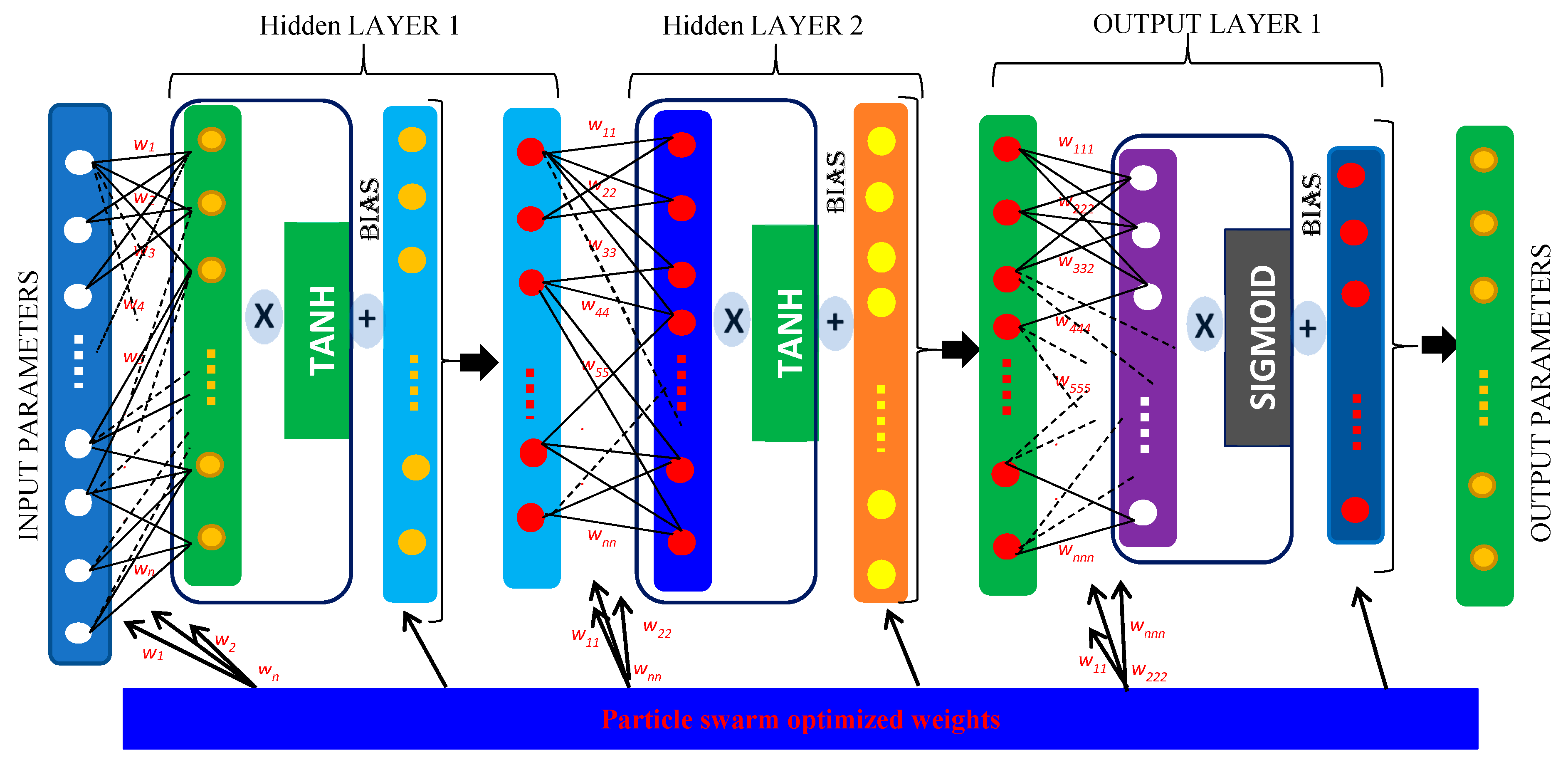
Despite the usefulness of PCA in dimensionality reduction and the original pattern retention for some new variables, it is also a useful tool for the determination of input variable significance and influence on the output variable [29]. The implementation of PCA transformation in this study does not only help in dimensionality reduction but in the transformation of the variables, which also enhances the hyperspace for the optimal combination of the hyperparameters. To ensure that the model variables are optimized in the FFANN, PSO was introduced for iteratively obtaining the near perfect weights for the hidden layers of the network (Figure 2).
The PSO technique is used for obtaining the global maxima of the weights used in the search hyperspace of the algorithm by allowing the particles to move at their own velocities while adjusting to the velocities of other particles [30,31]. This procedure makes it possible to get the global best position of the particles per the relationship shown in Equation (3):
{ v i k + 1 = ω v i k + c 1 r 1 k ( P i k z i k ) + c 2 r 2 k ( P g k z i k ) z i k + 1 = z i k + v i k + 1
where vki represents the velocity of individual particle zki at an iteration k, r1 and r2 are random variables between 0 and 1, Pki is the best position of individual particle at k iteration, Pkg is the global best position of the swarm at k iteration, c1 and c2 are constants that represent the cognitive parameter and social parameter respectively and ω is the initial weight, which decreases linearly with the number of iterations per Equation (4) [31]:
ω k = ω m a x ( ω m a x ω m i n k m a x ) k
where ωmax and ωmin represent the maximum and minimum initial weights respectively and kmax represents the maximum number of iterations.
In the model, a set of observations of the input and output variables given by {(xi,yi)}i=1 of D dimensional feature vectors {xi ϵ ℝD} and ϒ corresponding outcomes {yi ϵ ℝϒ} were initially normalized using Equation (5) prior to the PCA transformation:
η n o r m = ( η η m i n η m a x η m i n )
where, ηnorm, η, ηmin and ηmax respectively represent the normalized, original, minimum and maximum values of the input or output variable.

2.2.1. Principal Component Analysis (PCA) Transformation

The normalized input and output variables given by {(x(n)i, y(n)i)}i=1, where PCA transformed from ℝ to ℝ dataspace using Equation (6) to Equation (7) [29]:
{ f x ( λ ( x ) ) = μ x + ν x λ ( x ) f y ( λ ( y ) ) = μ y + ν y λ ( y )
where fx and fy are the functions of the normalized input and output variables, µx, µy ϵ ℝ corresponds to the mean values of x(n) and y(n), whereas ν x and ν y are the ℓ × ℘ matrices with ℘ orthogonal unit vectors of the input and output variables respectively. The values λ(x) ϵ ℝ𝜈 and λ(y) ϵ ℝ𝜈 are the new dimensional datapoints projections of the normalized values of the input and output variables, which are expected to be less than or equal to the original datapoints.
Effective construction of the new PCA dimensions of the normalized input and output variables will involve minimizing the error value in k iterations per Equation (7).
{ min μ x , λ 1 , , k ( x ) , ν x i = 1 k x i ( n ) μ x ν x λ i ( x ) min μ y , λ 1 , , k ( y ) , ν y i = 1 k y i ( n ) μ y ν y λ i ( y )
The Singular Value Decomposition (SVD) technique has been employed for determining the principal components by some researchers who solved Equation (7) [32,33].

2.2.2. Feed-Forward Artificial Neural Network (FFANN) Modelling

To compute the output variables from the normalized and PCA transformed original values of the input variables, this model assumes that a nonlinear relationship exists between the input and output variables and uses the tanh and sigmoid (σ) activation functions shown in Equation (8) to convert the vectors multiplication values in the hidden layers and output layer shown in Figure 2.
{ tanh ( x ) = e ( x ) e ( x ) e ( x ) + e ( x ) σ ( x ) = 1 1 + e ( x )
Thus, the PCA-PSO-FFANN model for the output parameter as the normalized and PCA transformed input variables ( x i ( n p ) ) transverses through the hidden layers. The model for the various layers in the PCA-PSO-FFANN is determined with the relationships shown in Equations (9)–(12):
{ P r e a c t i v a t i o n   i n   i n p u t   l a y e r 1 : y i ( i n ) = W ( 1 ) x i ( n p ) + b ( 1 ) W ( 1 ) = [ W 1 ( 1 ) , W 2 ( 1 ) , , W ( 1 ) ] H ( 1 ) b ( 1 ) = [ b 1 ( 1 ) , b 2 ( 1 ) , , b H ( 1 ) ( 1 ) ] H ( 1 ) H ( 1 )
where W(1) represents the particle swarm optimized input weights at the input layer and b(1) is the bias at that layer, which is equivalent to the number of neurons in the hidden layer 1 given by H(1):
{ A c t i v a t i o n   i n   h i d d e n   l a y e r 1 : y i ( 1 ) = t a n h ( y ( i n ) ) P r e a c t i v a t i o n   i n   i n p u t   l a y e r 2 : y i ( 2 ) = W ( 2 ) + b ( 2 ) W ( 2 ) = [ W 1 ( 2 ) , W 2 ( 2 ) , , W H ( 2 ) ( 2 ) ] H ( 2 ) H ( 1 ) H ( 2 ) b ( 2 ) = [ b 1 ( 2 ) , b 2 ( 2 ) , , b H ( 2 ) ( 2 ) ] H ( 2 ) H ( 2 )
where W(2) represents the particle swarm optimized input weights at the hidden layer1 and b(2) is the bias at that layer, which is equivalent to the number of neurons in the hidden layer 2 given by H(2):
{ A c t i v a t i o n   i n   h i d d e n   l a y e r 2 : y i ( 3 ) = t a n h ( y ( 2 ) ) P r e a c t i v a t i o n   i n   i n p u t o u t p u t   l a y e r : y i ( 3 ) = W ( 3 ) + b ( 3 ) W ( 3 ) = [ W 1 ( 3 ) , W 2 ( 3 ) , , W H ( 2 ) ( 3 ) ] H ( 2 ) H ( 2 ) b ( 3 ) = [ b 1 ( 3 ) , b 2 ( 3 ) , , b ( 3 ) ]
where W(3) represents the particle swarm optimized input weights at the output layer and b(3) is the output layer bias, which is equivalent to the number of neurons in the output layer.
The estimated values of the output are computed by activating the result in Equation (11) with a sigmoidal activation function and adding the error value ɛ:
y i ( n p ) = σ ( y i ( 3 ) + ε ) .

2.3. PCA-Gradient Boosting Machine (GBM) Algorithm

GBM uses a learning procedure that involves the continuous building of new models in order to properly estimate the responses of the variables, by ensuring that the base-learners are maximally correlated with the negative gradient of the loss functions of the ensemble [34]. For a given experimental dataset {(xi,yi)}i=1 that is normalized and PCA transformed using Equation (6) to Equation (7), the GBM algorithm determined a functional dependency x ( n p ) f y ( n p ) for an ensemble estimator f ^ ( x ( n p ) ) that has a minimal loss function Ψ { y ( n p ) , f ( x ( n p ) ) } given by Equation (13) [35,36].
{ f ^ ( x ( n p ) ) = y ( n p ) f ^ ( x ( n p ) ) = arg min f ( x ( n p ) ) Ψ { y ( n p ) , f ( x ( n p ) ) }
If f ( x ( n p ) ) and f ^ ( x ( n p ) ) represent true functional dependency and estimated functional dependency respectively, and the parametric value of the track space of the relationships is restricted to the function f ( x ( n p ) , θ ) , then the function f ^ ( x ( n p ) ) shown in Equation (13) can be written per Equation (14).
{ f ^ ( x ( n p ) ) = f ( x ( n p ) , θ ^ ) f ^ ( x ( n p ) ) = a r g   min f ( x ( n p ) ) E x ( n p ) [ E y { Ψ { y ( n p ) , f ( x ( n p ) ) } | x ( n p ) ] θ ^ = a r g   min θ E x ( n p ) [ E y ( n p ) { Ψ { y ( n p ) , f ( x ( n p ) , θ ) } | x ( n p ) ]
where θ , θ ^ , E x ( n p ) and E y ( n p ) represent the set of parameters in the model, the set parameter estimates, expectation function of the explanatory variable and expectation function of the dependent variable, respectively.
Since solving Equation (14) in a numerical optimization is by iteration because of the absence of a closed form of the solution [34], the set parameter estimates θ ^ can be determined for k steps iteration as shown in Equation (15).
θ ^ = i = 1 k θ ^ i
The empirical loss function— J ( θ ) over the observed dataset ( x ( n p ) , x ( n p ) ) i = 1 can be determined with the step gradient descent following Equation (16) [34]:
J ( θ ) = i = 1 k Ψ ( y i ( n p ) , f ( x i ( n p ) , θ ^ ) ) .
Seeing that the improvement in the loss function gradient change— J ( θ ) gives rise to the optimized solution, the gradient of the loss function and the parametric estimate— θ ^ for a 1 to k steps interaction can be determined by using Equation (17):
{ J ( θ ) = { J ( θ i ) } = [ J ( θ ) J ( θ i ) ] θ = θ ^ k θ ^ k J ( θ )
where θ ^ k is the new incremental parameter estimate of the ensemble at a new iterative step k.

2.4. PCA-Random Forest (RF) Algorithm

Random forest is one of the ensemble learning procedures that generates numerous classifiers that are aggregated with a bagging technique and randomization to give extra weights to the nodes. This helps to enhance the prediction accuracy of the model via the bootstrapping of the sampled dataset [37,38,39]. By growing a set number of trees from the original dataset as bootstraps, budding unpruned classification trees and randomly selecting the best branches, new data are predicted from the trees.
The collection of the tree predictors— h ( x ( n p ) , θ k ) helps to minimize the individual prediction error of the trees for k = 1, …, k, the covariant of the PCA transformed training input variables—x(np) and θk, which is independent and identically distributed (iid) random vectors of the model parameter. The RF predictor uses unweighted averages over the collector ( h ^ ) shown in Equation (18) to generalize the prediction by minimizing the loss function and avoiding overfitting via the convergence of Equation (19) [40]:
h ^ ( x ( n p ) ) = 1 k k = 1 k h ( x ( n p ) , θ k )
E x ( n p ) , y ( n p ) ( y ( n p ) h ^ ( x ( n p ) ) ) 2 E x ( n p ) , y ( n p ) ( y ( n p ) E θ h ( x ( n p ) , θ ) ) 2 .
The loss function of the model has a least square formulation and is represented by E x ( n p ) , y ( n p ) ( y ( n p ) E θ h ( x ( n p ) , θ ) ) 2 , with E(*) being the expectation function of various parameters.

2.5. PCA-Deep Neural Network (DNN) Algorithm

The DNN uses a multilayer perceptron procedure to learn the pattern and behaviour of data with multiple levels of abstractions and applies a hierarchical architecture and backpropagation technique for minimizing error in the computation [41].
For a PCA transformed data— { x i ( n p ) , y i ( n p ) } i = 1 , a functional dependency f : R N { 0 , , L } that minimizes the loss function is determined by solving Equation (20):
{ Ψ { y ( n p ) , θ k } = i = 0 N I x ( n p ) , y ( n p ) I x ( n p ) , y ( n p ) = a r g   min k i = 1 N ( y ( n p ) ( x ( n p ) , θ k ) ) 2
where N is the number of training set and L is the number of labels.

3. Time-Dependent Reliability Modelling

The use of the MLAs described in the previous section to train a model for the instantaneous and time-dependent defect depth growth of the pipeline makes it possible to compute the failure probabilities and reliabilities. This scenario is attainable because the leak and burst failure susceptibility of the pipeline increases with the growth of the corrosion defect. Imperatively, the influences of the external forces resulting from the operational and environmental conditions of the pipeline bring about the reduction of the resistance of the asset to failure due to the increase in corrosion defect depth growth. To this end, the understanding and estimation of the status of the pipeline at any time will give the operators information for effective integrity management and risk reduction.
Since the reliability of the pipeline at any given time is the ability of the pipeline to efficiently transport the oil and gas from the fields without failure, and the failure is expected to occur when there is an extreme load on the asset, the time-dependent reliability is proposed as a function of the pipe-wall thickness loss. This is estimated with the operating conditions over a given time boundary. Although the limit state function has been utilized with the Monte Carlo simulation estimated failure rates for reliability assessment by numerous researchers [42,43], this reliance increased the subjectivity of the results. In this study, the level of uncertainty associated with the estimated reliability is reduced, as the rate of the pipe-wall thickness loss is based on the realistic estimates from the field operating conditions. Emphatically, the dependence of this model on the difference in the stress concentrations on the pipeline at zero corrosion defect depth, and the predicted corrosion defect depth at a given time, increases the accuracy of the computed reliability.
The reliability of the pipeline (R) at any given instance t can be determined with Equation (21), which has FR representing the cumulative density function, fR representing the probability density function and c and T standing for the mean pipe wall thickness loss function and the time to failure, respectively [44,45]:
R ( t ) = P r { T t } = 1 F R ( t ) = t f R ( c ) d c .
The rate of the pipe wall thickness loss λp(t) due to the corrosion can be estimated as a hazard function represented in Equation (22) [44].
{ λ p ( t ) = lim δ t 0 P r { t T t + δ t | T t } δ t λ p ( t ) = f R ( t ) R ( t )
If the rate of the pipe wall thickness loss is directly correlated with the probability of failure of the pipeline at a given time, and the probability of failure for 90% pipe-wall thickness loss is 1, the reliability, failure probability (fP) and the probability density function (fR) at any given time can be computed with Equations (23) and (24):
{ R ( t ) = e x p { 0 t f R ( c ) d c } R ( t ) = e x p { λ p t } f p = 1 e x p { λ p t }
f R ( t ) = λ p e x p { λ p t } .

4. Industrial Experiment and Application

To ascertain the functionality of the model developed in this study, field data from onshore oil and gas gathering pipelines were used. The dataset was obtained from fields in the Niger Delta region of Nigeria from sixty X52 grade pipelines for a period of ten years. The corrosion defect depths were measured with the pulse-echo technique of the Ultrasonic Thickness Measurement (UTM) while the operating parameters were routinely obtained from the fields over the period of monitoring. A comprehensive description of the experimental procedure can be obtained from the previous studies on the fields from references [12] and [46]. The descriptive statistics of the maximum values of the corrosion defect depths and the mean values of the operating parameters are summarized in Table 2.
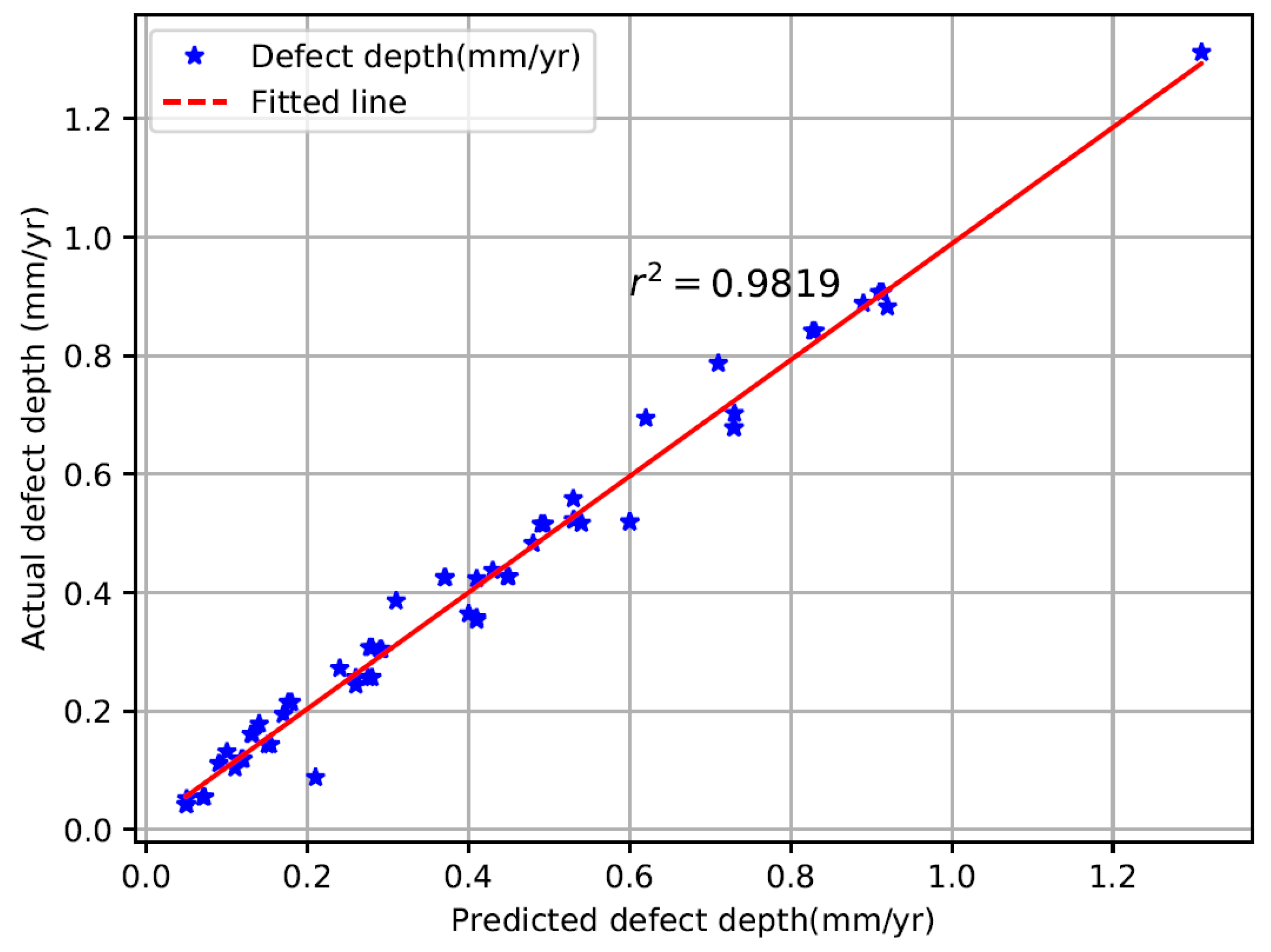
Due to the presence of missing values resulting from the unforeseen circumstances in the data collection procedure in the field, and the need to have a robust dataset for training, testing and validation of the model, a multivariate polynomial regression, Equation (25) was used to determine the relationship between the corrosion defect depth growth rate. A total of 60 wells of operating data from over 8300 records obtained over a period of ten years was used to develop the regression model by relying on the mean values of the maximum corrosion rates and the mean values of the operating parameters,
D d = α + i = 1 m β i ( 1 ) ϕ i + i = 1 m β i ( 2 ) ϕ i 2 + i = 1 m β i ( 3 ) ϕ i 2 + i = 1 m ρ ϕ i + ε
where β 1 , , m ( 1 ) , β 1 , , m ( 2 ) , β 1 , , m ( 3 ) and ρ are the coefficients of the operating parameters φ, φ2, φ3 and the product of φ, respectively, while Dd is the corrosion defect depth growth rate.
A comparison between the field measured corrosion defect depth growth rate and the ones predicted with Equation (25) is shown in Figure 3.
This polynomial model provided a baseline for generating the dataset for training the machine learning model as per the following procedures:
  • Randomly generate 20,000 uniform distribution of the operating parameters to sufficiently represent different data combinations of the operating parameters and corrosion defect depth growth.
  • Compute the corrosion defect depths growth rate based on Equation (25).
  • Randomly select 5000 samples of the corrosion defect depth and the operating parameters ensuring that the values are not more than ±25% of the original values. This variability is to give room for noises that are characteristics of field data operating in varying conditions. Since small changes in some of the operating parameters of the pipelines can result in corrosion defect growth changes [47,48,49], it is important to account for possible variation of the data beyond the original boundaries. This is vital for improving the quality of the model to cope with unexpected changes in the operating parameters characteristics and the attendant impact on the corrosion defect growth.
  • The dataset is used for training and validation in a 5-fold cross-ensemble validation training model having 20% of the original dataset for validation.
The model training was done in two phases, with phase one involving the PCA-PSO-FFANN and other PCA modified algorithms of GBM, DNN and RF. The second phase of the model training involved the same procedures and algorithms, but the datasets were not PCA transformed prior to the training. This second phase was used as a control for establishing the effect of the PCA transformation on the MLAs.
The PSO-FFANN algorithm was implemented with the cognitive (c1) and social parameter constants (c2) of 0.5, an initial weight (ω) of 0.9 and the best individual particle position (Pk) of 2.5, while using 100 particles and 1000 maximum iterations. The number of hidden neurons in the first and second layers of the FFANN was determined as 2* I_V + 4 and 2* I_V + 2, respectively, where I_V is the number of input variables to the model.

5. Results and Discussion

The comparison of the 5-fold cross-ensemble validation results of the PCA transformed dataset and the untransformed dataset was determined with the Root Mean Square Error (RMSE) and MAEP measurements shown in Table 3.
It can be seen from Table 3 that the performance of the algorithms with the PCA transformed dataset is better than those without the PCA transformation. The PCA transformation of the PSO-FFANN model resulted in an accuracy improvement of 4.3 times more than that obtained from the model prior to the PCA transformation of the dataset. The same case was noted with the PCA-GBM, PCA-RF and PCA-DNN that improved 5.32 times, 4.19 times and 3.52 times, respectively. These significant improvements in the accuracy of prediction with PCA transformations highlight the potency of the technique for machine learning and prediction of future states of corrosion defect depth growth. To further evaluate the performance of the PCA transformation, a dataset of simulated pipelines, obtained from Equation (25) (Table 4), that are corroding at low, mild, high and severe levels based on NACE classification [50], were modelled.
This simulation is important because the result shown in Table 3 is for pipelines whose corrosion defect depth comprises a mixture of low, mild, high and severe corrosion defect depth growth rates. Hence, understanding the behaviour of the model in different corrosion scenarios will be important in the determination of the robustness of the MLAs.
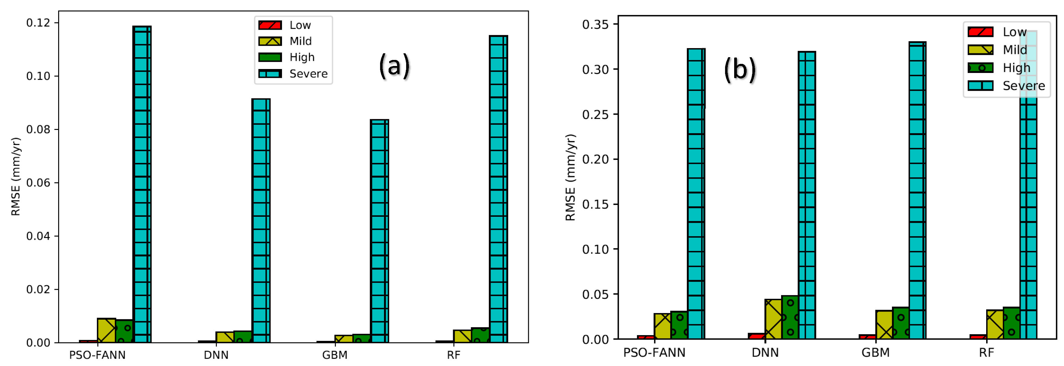
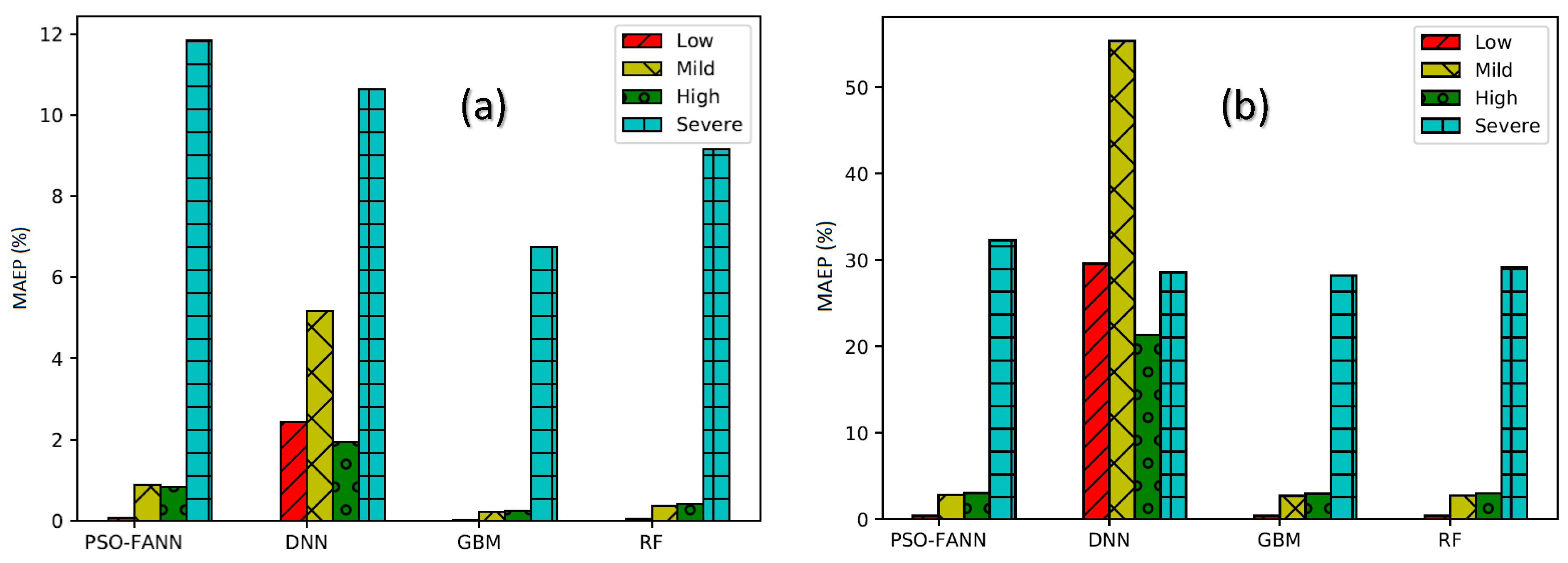
The performance of the algorithms, when the various classes of corrosion are considered on the pipelines as measured with the RMSE and MAEP, is shown in Figure 4 and Figure 5.
Again, it can be inferred from the information in Figure 4 and Figure 5 that the PCA transformed algorithms have superlative performance when compared with the algorithms with datasets that were untransformed. However, the accuracy of PCA transformed algorithms of the severe corrosion category is significantly lower than that of the other corrosion categories. PCA-DNN showed the worst accuracy level for the PCA transformed dataset when compared with the other models. However, the PCA-PSO-FFANN model did not perform better than the PCA-GBM and PCA-RF.

5.1. Estimation of the Instantaneous Defect Depth (IDD) and Time-Dependent Defect Depth (TDD) Growth

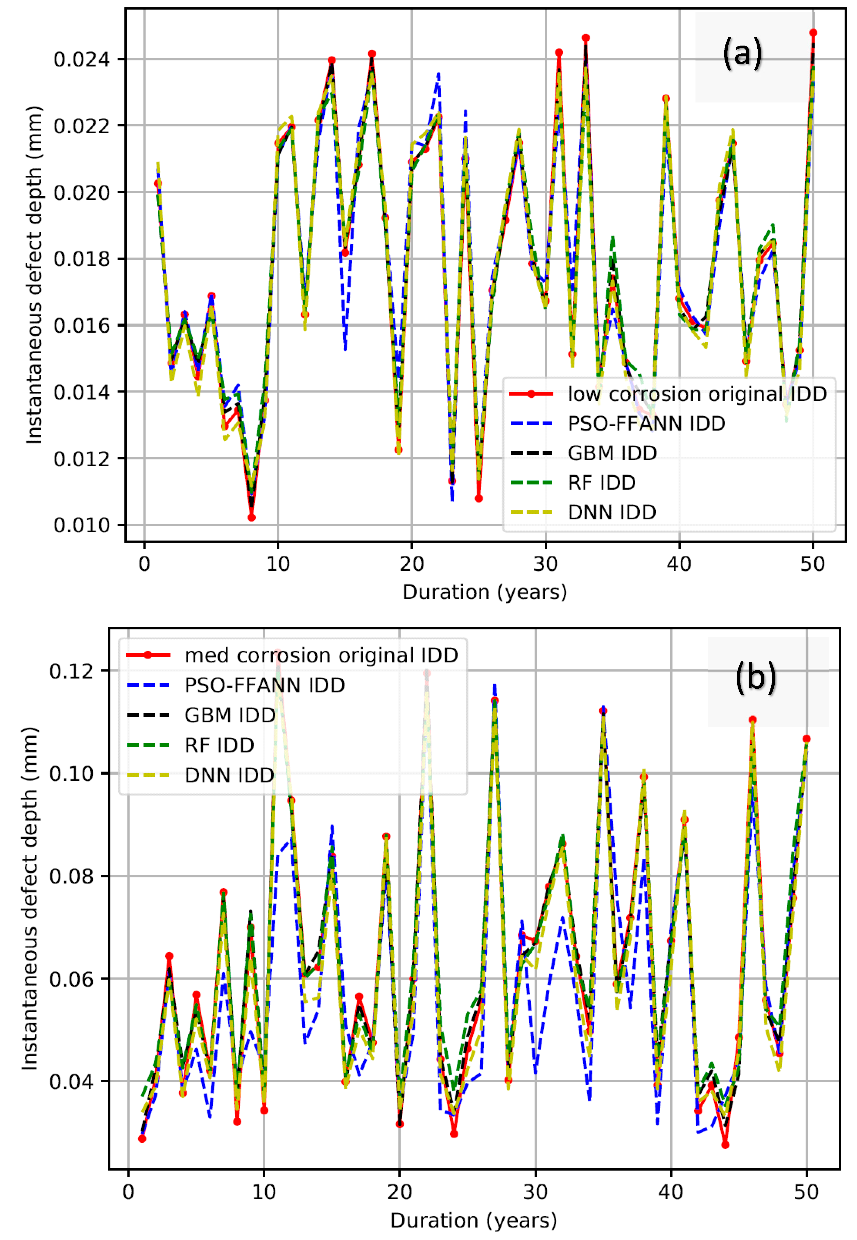
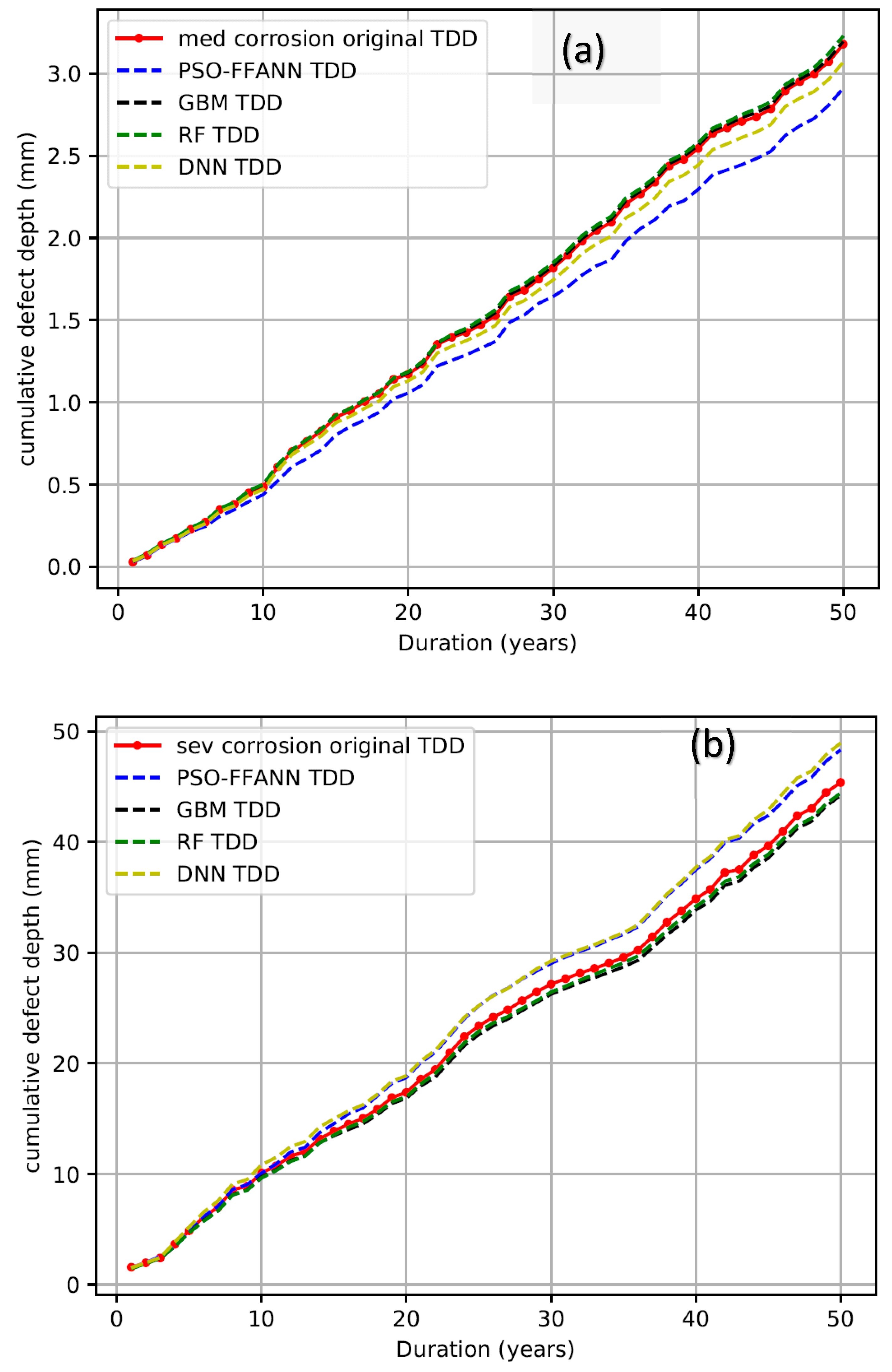
Since the IDD is vital for the estimation of the TDD growth and reliability estimation of the pipeline, as per the previous comments in this paper, the PCA algorithms are used for estimating the future corrosion defect behaviour of the corroded pipelines for different corrosion categories. For the pipelines with the corrosion defect depth characteristic shown in Table 4, the original simulated future instantaneous and time-dependent corrosion defects for a period of 50 years as exemplified with some of the corrosion categories are compared in Figure 6 and Figure 7.
Considering the fact that the status of a pipeline depends significantly on the corrosion defect depth growth at any given time, there is a high tendency to implement Corrosion Risk Assessment (CRA) of the pipelines with knowledge of this corrosion induced pipe wall thickness loss. The figures also indicated that the MLAs have predicted the low corrosion category better than the other categories, with PCA-GBM making a better prediction than the other algorithms. The prediction errors are most pronounced in the severe and mild corrosion categories, with PSO-FFANN and PCA-DNN showing a more distinctive lower accuracy of the predicted TDD growth than the other models.

5.2. Time-Dependent Reliability Estimation

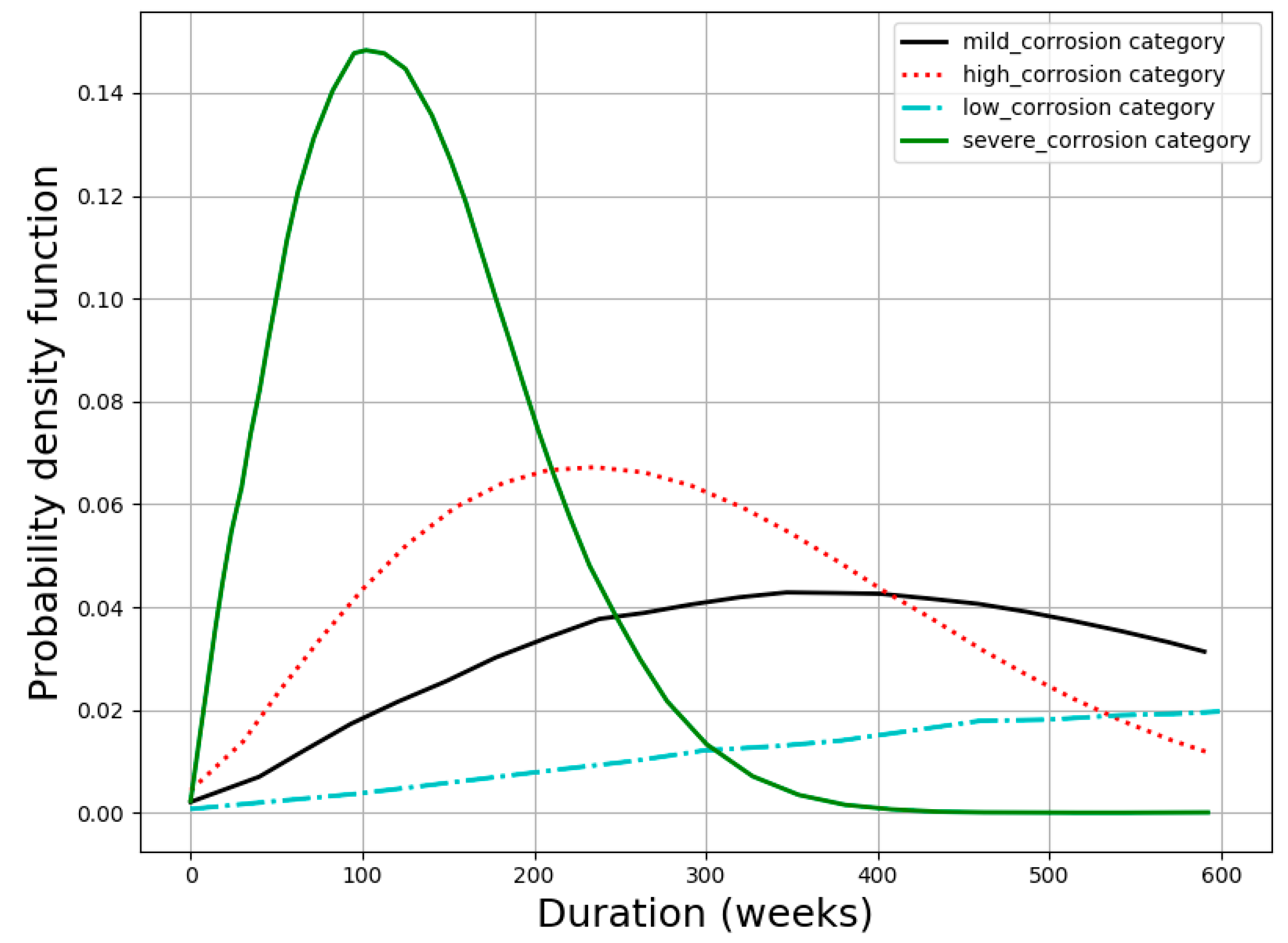
Considering the better prediction of the PCA transformed MLAs, and the comparatively more accurate prediction of the PCA-GBM than the PCA-PSO-FFANN and other MLAs (see Figure 4 and Figure 5), the model was used for estimating the time-dependent corrosion defect depth growth vis-à-vis the reliability of the pipelines. Based on the PCA-GBM and Equations (21)–(24), the probability density function, the probability of failure and the reliability of the pipelines undergoing different corrosion categories were determined (Figure 8, Figure 9 and Figure 10).
The right skewed tails of the probability density plots in Figure 8 give an indication of the degradation failure resulting from the loss of the pipe-wall thickness over time of the operation of the pipelines. Although the loss of pipe-wall thickness is the key to pipeline failure, the probability of the wear-off is significantly higher for the severe corrosion category than for any of the other categories. This extensively high wear-off probability for the severe corrosion category has been attributed to numerous factors that include the high concentration of the corrosive species from the reservoirs [28] and the microstructural flaws of the pipe material. It is expected that the corrosion deterioration rate of the pipelines will be higher at the early stages of the lifecycles of the pipelines but will gradually reduce with the ageing of the assets as the probability of failure gradually reduces (Figure 9). This phenomenon can be attributed to the passivity that results in the reduction of the electrochemical reactivities of the pipeline material in its environment, as protective films form on the corroded surfaces [4]. Although passivity can be short-lived due to erosion and turbulence in the pipelines [4], the prolonged complex interactions of the chemical species in the corrosive environment and the changing characteristics of the oil and gas flowing through the pipelines [2] can also contribute to the systematic inhibition reactions of the corrosive species.
The estimation of the failure probability and reliability of the pipelines will help pipeline integrity management since knowledge of the expected pipe-wall thickness loss will be a major trigger for different inspection, maintenance, repair and replacement operations. As expected, the pipelines with severe corrosion rates will be exposed to a higher risk of failure at a given time when compared with pipelines degrading at the other corrosion categories. For instance, from the information shown in Figure 10, it can be deduced that after 5 years of the pipeline service, it is expected that the low corroding pipeline will have a reliability of ~95%, the mildly corroded pipeline will be at ~78% reliability, the highly corroded pipeline will be at ~55% reliability and the pipeline undergoing severe corrosion will only have ~5% reliability. This variation in the reliabilities of the pipelines is very significant in asset integrity management. As such, the extracted knowledge from this machine learning algorithm will be effective in guiding corrosion mitigation strategies. To this end, fields that have very high corrosion tendencies could be managed with high priorities to reduce the risk of failure while prolonging the lifespan of the pipeline. This can be done through some specially planned integrity management programs, which can modify the characteristics of the operating parameters. Seeing that the corrosion risk level that an organization is willing to accept will depend on the failure probability at any instance, effective CRA can be designed and implemented in real-time following the modelled conditions of the pipeline at such instances.

6. Conclusions

The need to improve the accuracy of the estimated corrosion defect depth growth and the reliability of corroded and aged pipelines cannot be overemphasized, hence the need for developing a data-driven machine learning strategy for Corrosion Risk Assessment (CRA) of pipelines. Principal Component Analysis (PCA) and Particle Swarm Optimization (PSO) were used to develop ML models of corrosion defect growth. To establish the efficiency of the PCA in corrosion defect depth estimation, MLAs such as Gradient Boosting Machine (GBM), Random Forest (RF) and Deep Neural Network (DNN) were used for modelling corrosion defect depth growth after PCA transformation of the datasets.
Although, the PCA-PSO-FFANN algorithm and the other models, such as PCA-GBM, PCA-RF and PCA-DNN, were able to predict the corrosion datasets to a higher accuracy than the algorithms used for the modelling without PCA transformation, the PCA-GBM showed a superlative performance in comparison to the other algorithms. To this end, the PCA-GBM was used to implement a corrosion defect depth growth model of pipelines corroding at different categories: low (<0.025 mm/yr.), mild (0.025 mm/yr. to 0.13 mm/yr.), high (0.13 mm/yr. to 0.25 mm/yr.) and severe (>0.25 mm/yr.). By using the time-dependent corrosion defect depths growth rate estimated with the PCA-GBM and the hazard function-based failure probability and reliability models, the future status of the pipelines was determined.
This PCA-GBM model was tested with uniform corrosion datasets of onshore pipelines using the flow characteristics of the oil and gas and the water chemistry information from the reservoirs, which were obtained from routine quality control of the pipelines. Following these findings, it is possible to use the operating parameters of the pipelines over a given period to determine the status of the pipelines in the future, using a data-driven PCA-GBM machine learning algorithm. This algorithm will also enhance the real-time estimation of the corroded state of the aged pipelines since the technique can rely on historical information to estimate the future status of the corrosion defect depths. The reliability and failure probability estimation models will also help to enhance the integrity of the pipelines through short, medium and long-term integrity management planning. This will inevitable assist in the reduction of the failure risk of the pipelines, by ensuring that real-time inspection, maintenance, repairs and replacement of the ageing corroded pipelines are carried out.
Finally, the implementation of this model will help the operators of the oil and gas pipelines to:
  • Understand the expected time-dependent changes in the corrosion defect depth growth trajectory using the variabilities in the historical operating parameters and the corrosion defect depths growth rates.
  • Provide a handy tool for planning the pipeline integrity management by providing a guide to experts on the expected pipe wall thickness loss over a given time interval.
  • Give baseline information for effective management of the quality of the operating parameters, thereby maintaining a low cost of production in a safe operating environment.
  • Implement a microscale corrosion defect depth estimation since corrosion degradation in the pipeline is a continuous process, thereby opening a new frontier for quick and effective decisions on pipeline integrity management.

Funding

This research received no external funding.

Conflicts of Interest

The author declares no conflict of interest.

Data Availability

The results obtained in this paper are as obtained from the processed raw data.

References

  1. Ossai, C.I.; Boswell, B.; Davies, I.J. Pipeline failures in corrosive environments–A conceptual analysis of trends and effects. Eng. Fail. Anal. 2015, 53, 36–58. [Google Scholar] [CrossRef]
  2. Papavinasam, S.; Doiron, A.; Revie, R.W. Effect of surface layers on the initiation of internal pitting corrosion in oil and gas pipelines. Corrosion 2009, 65, 663–673. [Google Scholar] [CrossRef]
  3. Nordsveen, M.; Nešic, S.; Nyborg, R.; Stangeland, A. A mechanistic model for carbon dioxide corrosion of mild steel in the presence of protective iron carbonate films-Part 1: Theory and verification. Corrosion 2003, 59, 443–456. [Google Scholar] [CrossRef]
  4. Nešić, S. Key issues related to modelling of internal corrosion of oil and gas pipelines–A review. Corros. Sci. 2007, 49, 4308–4338. [Google Scholar] [CrossRef]
  5. Bazan, F.A.V.; Beck, A.T. Stochastic process corrosion growth models for pipeline reliability. Corros. Sci. 2013, 74, 50–58. [Google Scholar] [CrossRef]
  6. Melchers, R.E. Estimating uncertainty in maximum pit depth from limited observational data. Corros. Eng. Sci. Technol. 2010, 45, 240–248. [Google Scholar] [CrossRef]
  7. Melchers, R.E.; Jeffrey, R. Early corrosion of mild steel in seawater. Corros. Sci. 2005, 47, 1678–1693. [Google Scholar] [CrossRef]
  8. Nesic, S.; Postlethwaite, J. Relationship between the structure of disturbed flow and erosion-corrosion. Corrosion 1990, 46, 874–880. [Google Scholar] [CrossRef]
  9. Hu, X.; Neville, A. CO2 erosion–corrosion of pipeline steel (API X65) in oil and gas conditions—A systematic approach. Wear 2009, 267, 2027–2032. [Google Scholar] [CrossRef]
  10. Sheikh, A.K.; Boah, J.K.; Hansen, D.A. Statistical modeling of pitting corrosion and pipeline reliability. Corrosion 1990, 46, 190–197. [Google Scholar] [CrossRef]
  11. Caleyo, F.; Velázquez, J.C.; Valor, A.; Hallen, J.M. Markov chain modelling of pitting corrosion in underground pipelines. Corros. Sci. 2009, 51, 2197–2207. [Google Scholar] [CrossRef]
  12. Ossai, C.I.; Boswell, B.; Davies, I. Markov chain modelling for time evolution of internal pitting corrosion distribution of oil and gas pipelines. Eng. Fail. Anal. 2016, 60, 209–228. [Google Scholar] [CrossRef]
  13. Cai, J.; Cottis, R.A.; Lyon, S.B. Phenomenological modelling of atmospheric corrosion using an artificial neural network. Corros. Sci. 1999, 41, 2001–2030. [Google Scholar] [CrossRef]
  14. Abbas, M.H.; Norman, R.; Charles, A. Neural network modelling of high-pressure CO2 corrosion in pipeline steels. Process Saf. Environ. Prot. 2018, 119, 36–45. [Google Scholar] [CrossRef]
  15. Arzaghi, E.; Abbassi, R.; Garaniya, V.; Binns, J.; Chin, C.; Khakzad, N.; Reniers, G. Developing a dynamic model for pitting and corrosion-fatigue damage of subsea pipelines. Ocean Eng. 2018, 150, 391–396. [Google Scholar] [CrossRef]
  16. De Masi, G.; Vichi, R.; Gentile, M.; Bruschi, R.; Gabetta, G. A Neural Network Predictive Model of Pipeline Internal Corrosion Profile. In Proceedings of the IEEE SIMS, Washington, DC, USA, 29 April–1 May 2014. [Google Scholar]
  17. Askari, M.; Aliofkhazraei, M.; Ghaffari, S.; Hajizadeh, A. Film former corrosion inhibitors for oil and gas pipelines—A technical review. J. Nat. Gas Sci. Eng. 2018, 58, 92–114. [Google Scholar] [CrossRef]
  18. Cheng, A.; Chen, N.-Z. Corrosion fatigue crack growth modelling for subsea pipeline steels. Ocean Eng. 2017, 142, 10–19. [Google Scholar] [CrossRef]
  19. Dann, M.R.; Maes, M.A. Stochastic corrosion growth modeling for pipelines using mass inspection data. Reliab. Eng. Syst. Saf. 2018, 180, 245–254. [Google Scholar] [CrossRef]
  20. Velázquez, J.C.; Cruz-Ramirez, J.C.; Valor, A.; Venegas, V.; Caleyo, F.; Hallen, J.M. Modeling localized corrosion of pipeline steels in oilfield produced water environments. Eng. Fail. Anal. 2017, 79, 216–231. [Google Scholar] [CrossRef]
  21. Jančíková, Z.; Zimný, O.; Koštial, P. Prediction of metal corrosion by neural networks. Metalurgija 2013, 52, 379–381. [Google Scholar]
  22. Kenny, E.D.; Paredes, R.S.; de Lacerda, L.A.; Sica, Y.C.; de Souza, G.P.; Lázaris, J. Artificial neural network corrosion modeling for metals in an equatorial climate. Corros. Sci. 2009, 51, 2266–2278. [Google Scholar] [CrossRef]
  23. Cheng, Y.; Huang, W.L.; Zhou, C.Y. Artificial neural network technology for the data processing of on-line corrosion fatigue crack growth monitoring. Int. J. Press. Vessel. Pip. 1999, 76, 113–116. [Google Scholar] [CrossRef]
  24. Singer, M. Top-of-the-line corrosion. In Trends in Oil and Gas Corrosion Research and Technologies; Woodhead Publishing: Cambridge, Sawston, UK, 2017; pp. 385–408. [Google Scholar]
  25. Boyun, G.; Xinghui, L.; Xuehao, T. Chapter 22—Pipeline Pigging. Petroleum Production Engineering, 2nd ed.; Boyun, G., Xinghui, L., Xuehao, T., Eds.; Gulf Professional Publishing: Oxford, UK, 2017; pp. 701–720. ISBN 9780128093740. [Google Scholar] [CrossRef]
  26. Nianzhong, L.; Kaiming, C.; Jianhua, F. Intelligent Pigging Technology and Application for Gas Pipelines. Nat. Gas Ind. 2005, 25, 116. [Google Scholar]
  27. Yu, B.; Li, D.Y.; Grondin, A. Effects of the dissolved oxygen and slurry velocity on erosion–corrosion of carbon steel in aqueous slurries with carbon dioxide and silica sand. Wear 2013, 302, 1609–1614. [Google Scholar] [CrossRef]
  28. Zhu, X.Y.; Lubeck, J.; Kilbane, J.J. Characterization of microbial communities in gas industry pipelines. Appl. Environ. Microbiol. 2003, 69, 5354–5363. [Google Scholar] [CrossRef]
  29. Abdi, H.; Williams, L.J. Principal component analysis. Wiley interdisciplinary reviews: Comput. Stat. 2010, 2, 433–459. [Google Scholar] [CrossRef] [Green Version]
  30. Coulibaly, P.; Baldwin, C.K. Nonstationary Hydrological Time Series Forecasting Using Nonlinear Dynamic Methods. J. Hydrol. 2005, 307, 174–307. [Google Scholar] [CrossRef]
  31. Shi, Y.; Eberhart, R.C. A Modified Particle Swarm Optimizer. In Proceedings of the IEEE International Conference on Evolutionary Computation, Anchorage, AK, USA, 4–9 May 1988; pp. 69–73. [Google Scholar]
  32. Wall, M.E.; Rechtsteiner, A.; Rocha, L.M. Singular value decomposition and principal component analysis. In A Practical Approach to Microarray Data Analysis; Springer: Boston, MA, USA, 2003; pp. 91–109. [Google Scholar]
  33. Lagerlund, T.D.; Sharbrough, F.W.; Busacker, N.E. Spatial filtering of multichannel electroencephalographic recordings through principal component analysis by singular value decomposition. J. Clin. Neurophysiol. 1997, 14, 73–82. [Google Scholar] [CrossRef]
  34. Natekin, A.; Alois, K. Gradient Boosting Machines, a Tutorial. Front. Neurorobotics 2013, 7, 21. [Google Scholar] [CrossRef]
  35. Friedman, J.H. Greedy Function Approximation: A Gradient Boosting Machine. Ann. Stat. 2001, 29, 1189–1232. [Google Scholar] [CrossRef]
  36. Ridgeway, G. Generalized Boosted Models: A Guide to the gbm Package. Update 1.1. 2007. Available online: http://btr0x2.rz.uni-bayreuth.de/math/statlib/R/CRAN/doc/vignettes/gbm/gbm.pdf (accessed on 15 December 2019).
  37. Chen, L.; Cheng, X. Classification of High-resolution Remotely Sensed Images Based on Random Forests. J. Softw. Eng. 2016, 10, 318–327. [Google Scholar] [CrossRef]
  38. Breiman, L. Bagging predictors. Mach. Learn. 1996, 24, 123–140. [Google Scholar] [CrossRef] [Green Version]
  39. Breiman, L. Random forests. Mach. Learn. 2001, 45, 5–32. [Google Scholar] [CrossRef]
  40. Segal, M.R. Machine Learning Benchmarks and Random Forest Regression; Center for Bioinformatics and Molecular Biostatistics: UC San Francisco, CA, USA, 2004; Available online: https://escholarship.org/uc/item/35x3v9t4 (accessed on 12 January 2019).
  41. Brillante, L.; Gaiotti, F.; Lovat, L.; Vincenzi, S.; Giacosa, S.; Torchio, F.; Segade, S.R.; Rolle, L.; Tomasi, D. Investigating the use of gradient boosting machine, random forest and their ensemble to predict skin flavonoid content from berry physical–mechanical characteristics in wine grapes. Comput. Electron. Agric. 2015, 117, 186–193. [Google Scholar] [CrossRef]
  42. Ahammed, M. Probabilistic estimation of remaining life of a pipeline in the presence of active corrosion defects. Int. J. Press. Vessel. Pip. 1998, 75, 321–329. [Google Scholar] [CrossRef]
  43. Caleyo, F.; Gonzalez, J.L.; Hallen, J.M. A study on the reliability assessment methodology for pipelines with active corrosion defects. Int. J. Press. Vessel. Pip. 2002, 79, 77–86. [Google Scholar] [CrossRef]
  44. Rausand, M.; Høyland, A. System Reliability Theory: Models, Statistical Methods, and Applications; John Wiley & Sons: Hoboken, NJ, USA, 2004; Volume 396. [Google Scholar]
  45. Akpan, U.O.; Koko, T.S.; Ayyub, B.; Dunbar, T.E. Risk assessment of aging ship hull structures in the presence of corrosion and fatigue. Mar. Struct. 2002, 15, 211–231. [Google Scholar] [CrossRef]
  46. Ossai, C.I.; Boswell, B.; Davies, I.J. Predictive modelling of internal pitting corrosion of aged non-piggable pipelines. J. Electrochem. Soc. 2015, 162, C251–C259. [Google Scholar] [CrossRef]
  47. Nesic, S.; Lee, K.L.J.; Ruzic, V. A Mechanistic Model of Iron Carbonate Film Growth and the Effect on Co2 Corrosion of Mild Steel; CORROSION/2002, paper; 02237; NACE International: Houston, TX, USA, 2002. [Google Scholar]
  48. Mora-Mendoza, J.L.; Turgoose, S. Fe3C influence on the corrosion rate of mild steel in aqueous CO2 systems under turbulent flow conditions. Corros. Sci. 2002, 44, 1223–1246. [Google Scholar] [CrossRef]
  49. Wang, Y.; Cheng, G.; Wu, W.; Qiao, Q.; Li, Y.; Li, X. Effect of pH and chloride on the micro-mechanism of pitting corrosion for high strength pipeline steel in aerated NaCl solutions. Appl. Surf. Sci. 2015, 349, 746–756. [Google Scholar] [CrossRef]
  50. NACE Standard RP0775, Preparation, Installation, Analysis and Interpretation of Corrosion Coupons in Oilfield Operations; NACE International: Houston, TX USA, 2005.
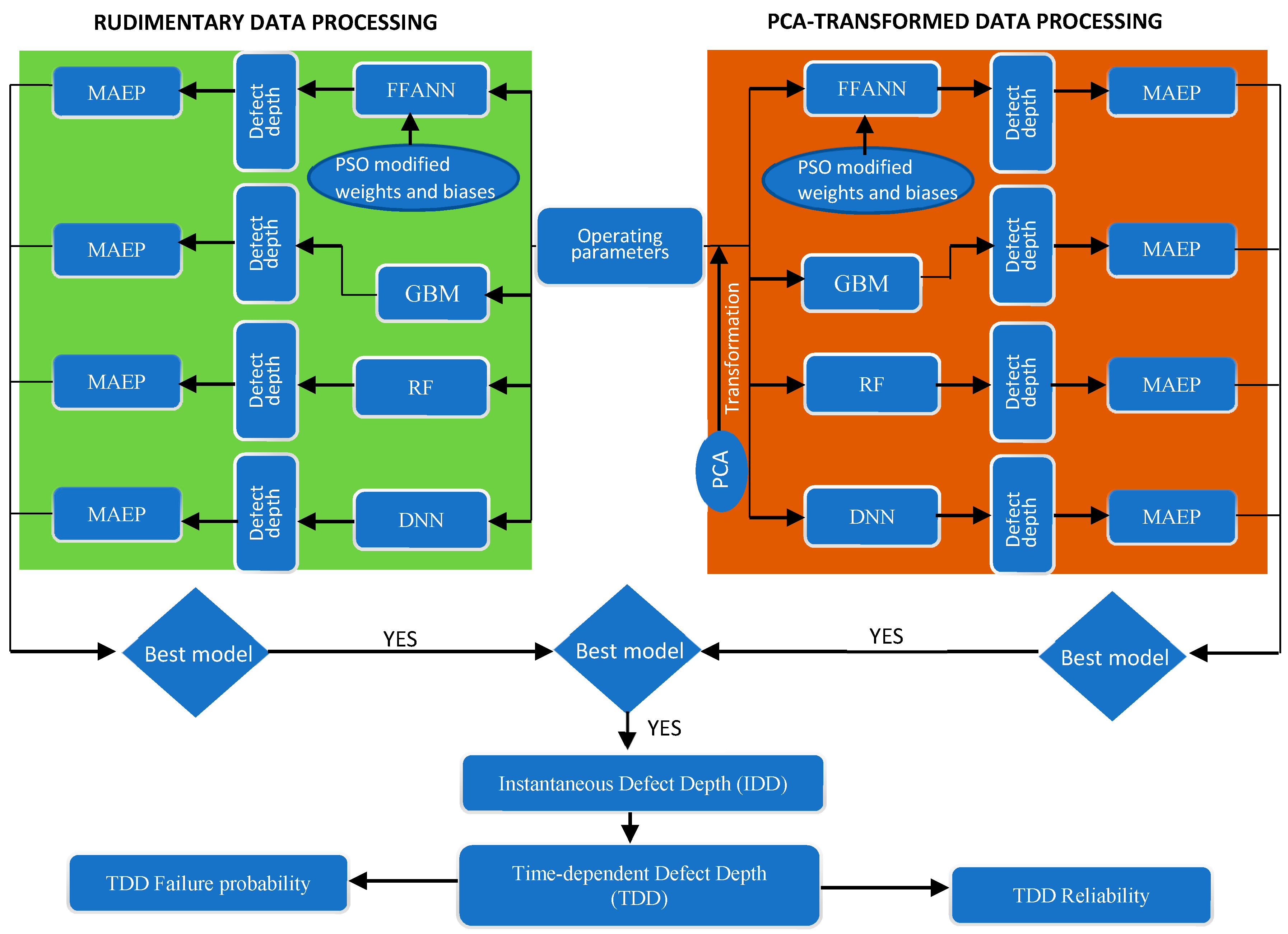
Figure 1. Schematic of the data-driven technique for corrosion Risk Assessment (CRA) of aged corroded pipelines (FFANN: Feed-Forward Artificial Neural Network; PCA: Principal Component Analysis; GBM: Gradient Boosting Machine; RF: Random Forest; PSO: Particle Swarm optimization; MAEP: Mean Absolute Error Percentage).
Bdcc 03 00028 g001
Figure 2. Framework for the particle swarm optimization of the feed-forward artificial neural network model.
Bdcc 03 00028 g002
Figure 3. Comparison of the field measured corrosion defect depth with that estimated with Equation (25).
Bdcc 03 00028 g003
Figure 4. Comparison of the RMSE of the PCA transformed and untransformed datasets of low, mild, high and severe corroding pipelines—(a): PCA transformed dataset; (b): Untransformed dataset.
Bdcc 03 00028 g004
Figure 5. Comparison of the MAEP of the PCA transformed and untransformed datasets of low, mild, high and severe corroding pipelines—(a): PCA transformed dataset; (b): Untransformed dataset.
Bdcc 03 00028 g005
Figure 6. Comparison of the Instantaneous Defect Depth (IDD) of pipelines undergoing low, mild, high and severe corrosion categories—(a): low corrosion; (b): mild corrosion.
Bdcc 03 00028 g006
Figure 7. Comparison of Time-dependent Defect Depth (TDD) of pipelines undergoing low, mild, high and severe corrosion categories—(a): mild corrosion; (b): severe corrosion.
Bdcc 03 00028 g007
Figure 8. PCA-GBM estimated time-dependent probability density function of the pipelines undergoing low, mild, high and severe corrosion categories.
Bdcc 03 00028 g008
Figure 9. PCA-GBM estimated Time-dependent probability of failure of the pipelines undergoing low, mild, high and severe corrosion categories.
Bdcc 03 00028 g009
Figure 10. PCA-GBM estimated Time-dependent reliability of the pipelines undergoing low, mild, high and severe corrosion categories.
Bdcc 03 00028 g010
Table 1. Input variables used for the determination of the corrosion defect depth of the pipelines.
Input VariableDescriptionUnitRemark
TMTemperature°CWater chemistry
PCO2CO2 Partial PressureMPa
pHpH
SO4sulphate ion concentrationg/ml
CLchloride ion concentrationg/ml
FEiron contentg/ml
HCO3Total Alkalinity as HCO3g/ml
PSOperating pressurepsi
CACalcium concentrationg/ml
BSWBasic sediment and water%Flow characteristics
MMCFDMillion Cubic Feet per day of gasmmcfd
BOPDBarrel of Oil production per daybbl/day
BWPDBarrel of Water production per daybbl/day
Table 2. Descriptive statistics of the studied parameters.
VariableDescriptionUnitMeanst. devMinMax
TMTemperature°C45.9817.292174
PCO2CO2 Partial PressureMPa0.130.10.010.61
pHpH7.60.646.218.57
SOsulphate ion concentrationg/mL34.3120.37270
CLchloride ion concentrationg/mL3168.792382.86667571.14
BSWBasic sediment and water%0.420.340.010.9
MMCFDMillion Cubic Feet per day of gasmmcfd8.545.170.217.54
BOPDBarrel of Oil production per daybbl/day684.48337.451251565.97
BWPDBarrel of Water production per daybbl/day1269.381965.9619328
FEiron contentg/mL1.170.970.042.79
HCO3Total Alkalinity as HCO3g/mL2404.931161.44152.54209
PSoperating pressurepsi880.93569.82652050
CACalcium concentrationg/mL1.110.790.022.56
DdMax defect depth ratemm/yr.0.40.280.051.31
Table 3. Summary of the Root Mean Square Error (RMSE) and Mean Absolute Error Percentage (MAEP) values of the MLAs for the PCA transformed and Untransformed datasets (std: standard deviation).
AlgorithmOriginal Data without TransformationPCA Transformed
RMSEMAEPRMSEMAEP
MeanstdMeanstdMeanstdMeanstd
PSO-FFANN0.41170.014634.13291.37740.096010.01187.85881.1361
GBM0.3770.005431.92660.79060.07650.0036.00820.13334
RF0.38510.0132.42670.99190.09730.00217.74210.099
DNN0.29630.034323.6472.4270.07880.02776.68132.4862
Table 4. Summary of the corrosion defect depths growth rate of the pipelines degrading at different corrosion categories.
Corrosion CategoryMeanStdMinMax
low0.0180.0040.010.025
Mild0.0770.0310.0250.13
High0.1890.0340.130.25
Severe0.880.3780.2511.57