Mining Temporal Patterns to Discover Inter-Appliance Associations Using Smart Meter Data

Abstract
1. Introduction
2. Related Work
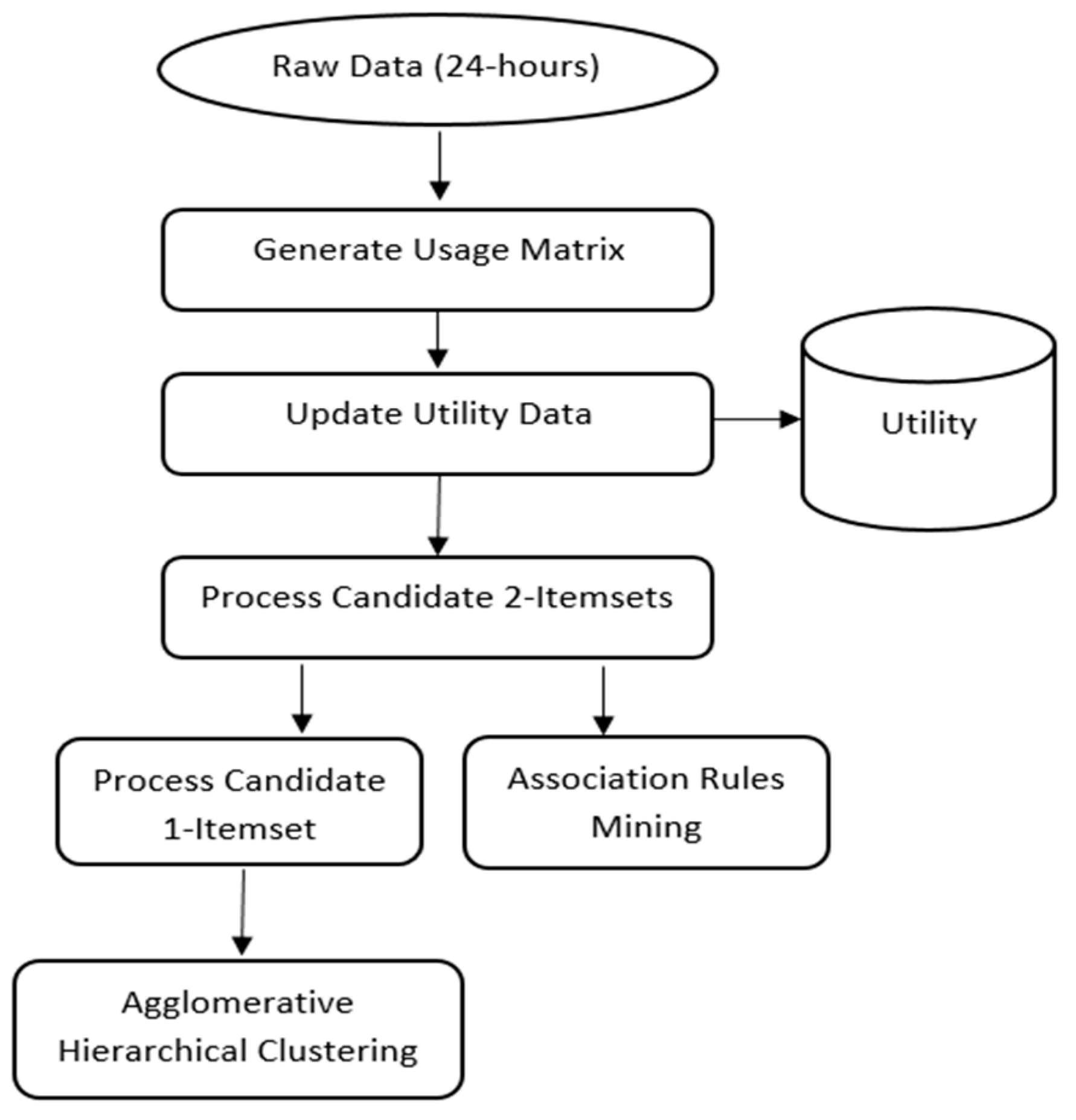
3. Proposed Methodology
- Data Preparation.
- Calculating Appliances’ Utility.
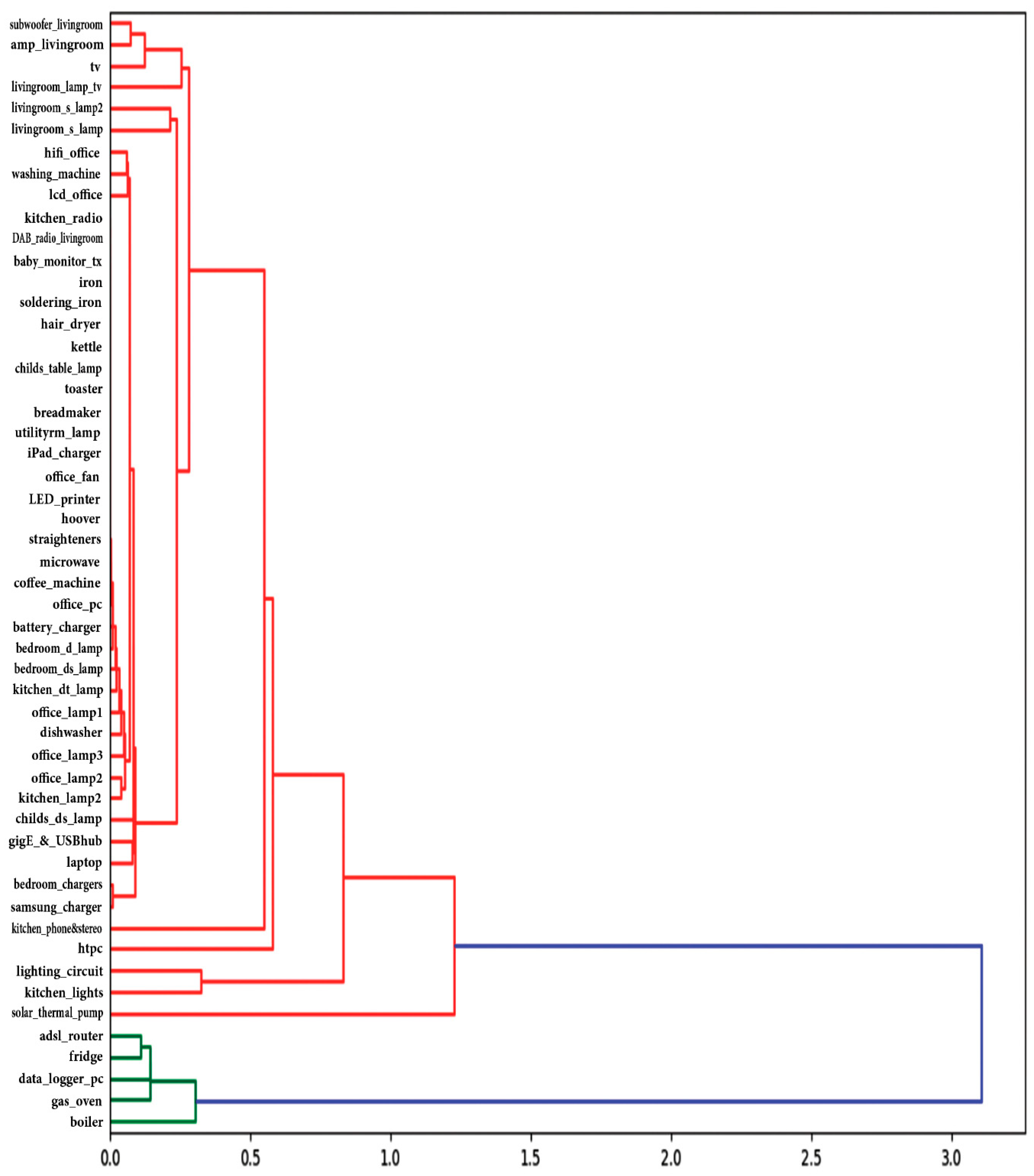
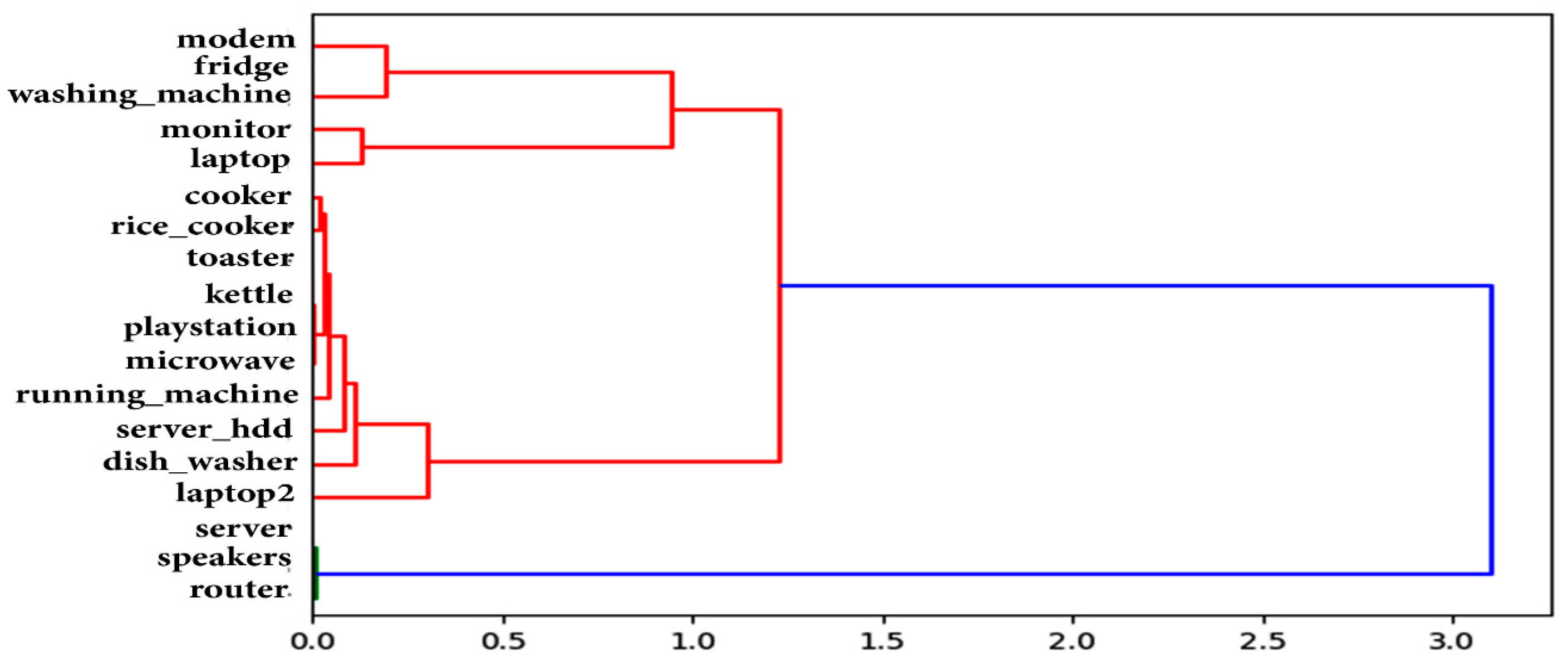
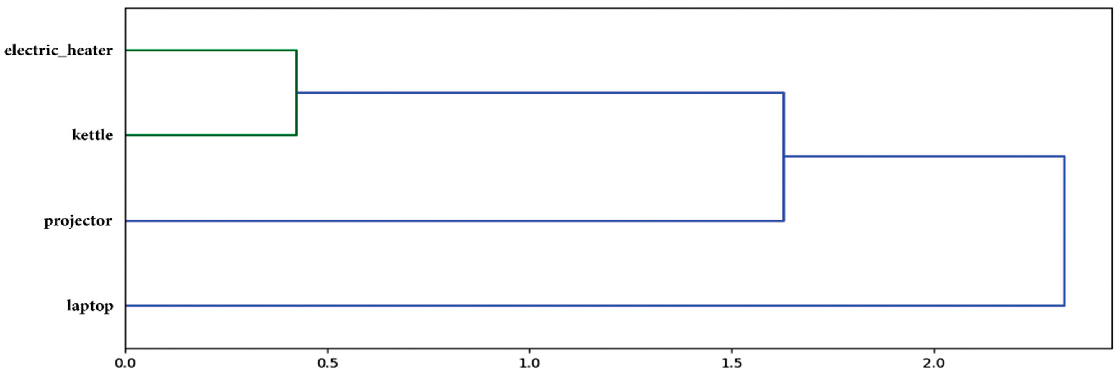
- Extracting Appliance–Appliance Association.
3.1. Data Preparation
3.2. Calculating Appliances’ Utility
3.3. Extracting Appliance–Appliance Associations
| Algorithm 1 Extracting Appliances Temporal Utility |
| Require: minimum support minsup Ensure: Utility-Oriented Temporal Association s 1: candidate2 ← generate candidate 2-itemsets 2: for each item(a1, a2) ∈ candidate2 do 3: for each hour(h) ∈ 24-h do 4: activeDays ← days having item active in hour 5: length ← length(activeDays) 6: if length > 0 then 7: item.startAth ← date of the first active day 8: item.endAth ← date of the last active day 9: item.FUh ← length 10: item.Uh ← calculated using Equation (5) 11: item.FTUh ← calculated using Equation (6) 12: item.selectedh ← item.FTUh > minsup 13: if item.selectedh then 14: a1.FTUh ← calculated using Equation (6) 15: a2.FTUh ← calculated using Equation (6) 16: end if 17: end if 18: end for 19: end for |
| Algorithm 2: Generating Appliances’ Association Rules |
| Require: minimum support minsup, minimum confidence minconf, candidate 2-itemsets candidate2 Ensure: Appliances Association Rules 1: for each item(a1, a2) ∈ candidate2 do 2: for each hour(h) ∈ 24-h do 3: if a1.FTUh > minsup then 4: 5: 6: end if 11: if a2.FTUh > minsup then 4: 5: 6: end if 17: end for 18: end for |
4. Evaluation and Results
5. Conclusions and Future Work
Author Contributions
Funding
Conflicts of Interest
References
- Zhou, S.; Brown, M.A. Smart meter deployment in Europe: A comparative case study on the impacts of national policy schemes. J. Clean. Prod. 2017, 144, 22–32. [Google Scholar] [CrossRef]
- Bekara, C. Security issues and challenges for the IoT-based smart grid. Procedia Comput. Sci. 2014, 34, 532–537. [Google Scholar] [CrossRef]
- Palacios-García, E.J.; Guan, Y.; Savaghebi, M.; Vásquez, J.C.; Guerrero, J.M.; Moreno-Munoz, A.; Ipsen, B.S. Smart metering system for microgrids. In Proceedings of the 41st Annual Conference of the IEEE on Industrial Electronics Society (IECON), Yokohama, Japan, 9–12 November 2015; pp. 003289–003294. [Google Scholar]
- Albadi, M.H.; El-Saadany, E.F. A summary of demand response in electricity markets. Electr. Power Syst. Res. 2008, 78, 1989–1996. [Google Scholar] [CrossRef]
- Maragatham, G.; Lakshmi, M. UTARM: An efficient algorithm for mining of utility-oriented temporal association rules. Int. J. Knowl. Eng. Data Min. 2015, 3, 208–237. [Google Scholar] [CrossRef]
- Aghabozorgi, S.; Shirkhorshidi, A.S.; Wah, T.Y. Time-series clustering—A decade review. Inf. Syst. 2015, 53, 16–38. [Google Scholar] [CrossRef]
- Kelly, J.; Knottenbelt, W. The UK-DALE dataset, domestic appliance-level electricity demand and whole-house demand from five UK homes. Sci. Data 2015, 2, 150007. [Google Scholar] [CrossRef]
- Hassani, M.; Beecks, C.; Töws, D.; Seidl, T. Mining Sequential Patterns of Event Streams in a Smart Home Application. In Proceedings of the Lerner Wissen Adaption (LWA) Conference, Trier, Germany, 7–9 October 2015; pp. 159–170. [Google Scholar]
- Honarvar, A.R.; Sami, A. Extracting usage patterns from power usage data of homes’ appliances in smart home using big data platform. Int. J. Inf. Technol. Web Eng. 2016, 11, 39–50. [Google Scholar] [CrossRef]
- Rollins, S.; Banerjee, N. Using rule mining to understand appliance energy consumption patterns. In Proceedings of the 2014 IEEE International Conference on Pervasive Computing and Communications (PerCom), Budapest, Hungary, 24–28 March 2014; pp. 29–37. [Google Scholar]
- Ding, Y.; Borges, J.; Neumann, M.A.; Beigl, M. Sequential pattern mining—A study to understand daily activity patterns for load forecasting enhancement. In Proceedings of the 2015 IEEE First International Smart Cities Conference (ISC2), Guadalajara, Mexico, 25–28 October 2015; pp. 1–6. [Google Scholar]
- Zhang, X.; Kato, T.; Matsuyama, T. Learning a context-aware personal model of appliance usage patterns in smart home. In Proceedings of the 2014 IEEE Innovative Smart Grid Technologies-Asia (ISGT ASIA), Kuala Lumpur, Malaysia, 20–23 May 2014; pp. 73–78. [Google Scholar]
- Liao, Y.S.; Liao, H.Y.; Liu, D.R.; Fan, W.T.; Omar, H. Intelligent Power Resource Allocation by Context-Based Usage Mining. In Proceedings of the 2015 IIAI 4th International Congress on Advanced Applied Informatics, Okayama, Japan, 12–16 July 2015; pp. 546–550. [Google Scholar]
- Schweizer, D.; Zehnder, M.; Wache, H.; Witschel, H.F.; Zanatta, D.; Rodriguez, M. Using consumer behavior data to reduce energy consumption in smart homes: Applying machine learning to save energy without lowering comfort of inhabitants. In Proceedings of the 2015 IEEE 14th International Conference on Machine Learning and Applications (ICMLA), Miami, FL, USA, 9–11 December 2015; pp. 1123–1129. [Google Scholar]
- Chen, Y.C.; Peng, W.C.; Lee, W.C. A novel system for extracting useful correlation in smart home environment. In Proceedings of the 2013 IEEE 13th International Conference on Data Mining Workshops, Dallas, TX, USA, 7–10 December 2013; pp. 357–364. [Google Scholar]
- Chen, Y.C.; Chen, C.C.; Peng, W.C.; Lee, W.C. Mining correlation patterns among appliances in smart home environment. In Proceedings of the Pacific-Asia Conference on Knowledge Discovery and Data Mining, Tainan, Taiwan, 13–16 May 2014; pp. 222–233. [Google Scholar]
- Chen, Y.C.; Hung, H.C.; Chiang, B.Y.; Peng, S.Y.; Chen, P.J. Incrementally mining usage correlations among appliances in smart homes. In Proceedings of the 2015 18th International Conference on Network-Based Information Systems, Taipei, Taiwan, 2–4 September 2015; pp. 273–279. [Google Scholar]
- Singh, S.; Yassine, A. Mining energy consumption behavior patterns for households in smart grid. IEEE Trans. Emerg. Top. Comput. 2017. [Google Scholar] [CrossRef]
- McLoughlin, F.; Duffy, A.; Conlon, M. A clustering approach to domestic electricity load profile characterisation using smart metering data. Appl. Energy 2015, 141, 190–199. [Google Scholar] [CrossRef]
- Haben, S.; Singleton, C.; Grindrod, P. Analysis and clustering of residential customers energy behavioral demand using smart meter data. IEEE Trans. Smart Grid 2016, 7, 136–144. [Google Scholar] [CrossRef]
- Flath, C.; Nicolay, D.; Conte, T.; van Dinther, C.; Filipova-Neumann, L. Cluster analysis of smart metering data. Bus. Inf. Syst. Eng. 2012, 4, 31–39. [Google Scholar] [CrossRef]
- Benítez, I.; Quijano, A.; Díez, J.L.; Delgado, I. Dynamic clustering segmentation applied to load profiles of energy consumption from Spanish customers. Int. J. Electr. Power Energy Syst. 2014, 55, 437–448. [Google Scholar] [CrossRef]
- Kwac, J.; Flora, J.; Rajagopal, R. Household energy consumption segmentation using hourly data. IEEE Trans. Smart Grid 2014, 5, 420–430. [Google Scholar] [CrossRef]
- Cao, H.Â.; Beckel, C.; Staake, T. Are domestic load profiles stable over time? An attempt to identify target households for demand side management campaigns. In Proceedings of the 2013 39th Annual Conference of the IEEE Industrial Electronics Society (IECON), Vienna, Austria, 10–13 November 2013; pp. 4733–4738. [Google Scholar]
- Chelmis, C.; Kolte, J.; Prasanna, V.K. Big data analytics for demand response: Clustering over space and time. In Proceedings of the 2015 IEEE International Conference on Big Data (Big Data), Santa Clara, CA, USA, 29 October–1 November 2015; pp. 2223–2232. [Google Scholar]
- Quilumba, F.L.; Lee, W.J.; Huang, H.; Wang, D.Y.; Szabados, R.L. Using smart meter data to improve the accuracy of intraday load forecasting considering customer behavior similarities. IEEE Trans. Smart Grid 2015, 6, 911–918. [Google Scholar] [CrossRef]
- Al-Otaibi, R.; Jin, N.; Wilcox, T.; Flach, P. Feature construction and calibration for clustering daily load curves from smart-meter data. IEEE Trans. Ind. Inform. 2016, 12, 645–654. [Google Scholar] [CrossRef]
- Gajowniczek, K.; Ząbkowski, T. Data mining techniques for detecting household characteristics based on smart meter data. Energies 2015, 8, 7407–7427. [Google Scholar] [CrossRef]
- Adika, C.O.; Wang, L. Autonomous appliance scheduling based on time of use probabilities and load clustering. In Proceedings of the 2012 10th International Power & Energy Conference (IPEC), Ho Chi Minh City, Vietnam, 12–14 December 2012; pp. 42–47. [Google Scholar]
- Ale, J.M.; Rossi, G.H. An approach to discovering temporal association rules. In Proceedings of the 2000 ACM Symposium on Applied Computing-Volume 1, Como, Italy, March 19–21 2000; pp. 294–300. [Google Scholar]
- Zida, S.; Fournier-Viger, P.; Lin, J.C.; Wu, C.W.; Tseng, V.S. EFIM: A highly efficient algorithm for high-utility itemset mining. In Proceedings of the Mexican International Conference on Artificial Intelligence, Cuernavaca, Mexico, 25–31 October 2015; pp. 530–546. [Google Scholar]
- Srikant, R.; Vu, Q.; Agrawal, R. Mining association rules with item constraints. In Proceedings of the Third Conference on Knowledge Discovery in Databases and Data Mining (KDD), Newport Beach, CA, USA, 14–17 August 1997; pp. 67–73. [Google Scholar]
- Chai, B.; Chen, J.; Yang, Z.; Zhang, Y. Demand response management with multiple utility companies: A two-level game approach. IEEE Trans. Smart Grid 2014, 5, 722–731. [Google Scholar] [CrossRef]
- Apostolopoulos, P.A.; Tsiropoulou, E.E.; Papavassiliou, S. Demand response management in smart grid networks: A two-stage game-theoretic learning-based approach. Mob. Netw. Appl. 2018, 1–14. [Google Scholar] [CrossRef]


| Association Rule | Confidence | Hour | From (dd-mm-yy) | To (dd-mm-yy) |
|---|---|---|---|---|
| kitchen_lights ⟹ tv | 96% | 22 | 2-1-2013 | 22-4-2017 |
| kitchen_lights ⟹ tv | 96% | 23 | 9-1-2013 | 25-4-2017 |
| tv ⟹ amp_livingroom | 100% | 0 | 1-1-2013 | 22-4-2017 |
| tv ⟹ amp_livingroom | 100% | 20 | 1-1-2013 | 25-4-2017 |
| tv ⟹ amp_livingroom | 100% | 21 | 1-1-2013 | 25-4-2017 |
| tv ⟹ amp_livingroom | 100% | 22 | 1-1-2013 | 25-4-2017 |
| tv ⟹ amp_livingroom | 100% | 23 | 1-1-2013 | 25-4-2017 |
| amp_livingroom ⟹ tv | 92% | 0 | 1-1-2013 | 22-4-2017 |
| amp_livingroom ⟹ tv | 91% | 21 | 1-1-2013 | 25-4-2017 |
| amp_livingroom ⟹ tv | 97% | 22 | 1-1-2013 | 25-4-2017 |
| amp_livingroom ⟹ tv | 96% | 23 | 1-1-2013 | 25-4-2017 |
| tv ⟹ subwoofer_livingroom | 91% | 0 | 1-1-2013 | 22-4-2017 |
| tv ⟹ subwoofer_livingroom | 100% | 20 | 1-1-2013 | 25-4-2017 |
| tv ⟹ subwoofer_livingroom | 98% | 21 | 1-1-2013 | 25-4-2017 |
| tv ⟹ subwoofer_livingroom | 95% | 22 | 1-1-2013 | 25-4-2017 |
| tv ⟹ subwoofer_livingroom | 94% | 23 | 1-1-2013 | 25-4-2017 |
| subwoofer_livingroom ⟹ tv | 90% | 0 | 13-3-2013 | 22-4-2017 |
| subwoofer_livingroom ⟹ tv | 91% | 21 | 12-3-2013 | 25-4-2017 |
| subwoofer_livingroom ⟹ tv | 99% | 22 | 12-3-2013 | 25-4-2017 |
| subwoofer_livingroom ⟹ tv | 97% | 23 | 12-3-2013 | 25-4-2017 |
| Association Rule | Confidence | Hour | From (dd-mm-yy) | To (dd-mm-yy) |
|---|---|---|---|---|
| laptop ⟹ monitor | 90–96% | 0-23 | 17-2-2013 | 10-10-2013 |
| monitor ⟹ laptop | 98–100% | 0-23 | 17-2-2013 | 10-10-2013 |
| laptop2 ⟹ laptop | 95% | 21 | 17-4-2013 | 9-10-2013 |
| laptop2 ⟹ laptop | 89% | 22 | 17-4-2013 | 9-10-2013 |
| laptop2 ⟹ laptop | 100% | 23 | 17-4-2013 | 9-10-2013 |
| laptop ⟹ modem | 89% | 9 | 22-3-2013 | 6-10-2013 |
| laptop ⟹ modem | 78% | 10 | 1-3-2013 | 6-10-2013 |
| modem ⟹ laptop | 79% | 22 | 21-5-2013 | 9-10-2013 |
| modem ⟹ laptop | 84% | 23 | 20-5-2013 | 9-10-2013 |
| laptop2 ⟹ monitor | 89% | 21 | 17-4-2013 | 9-10-2013 |
| laptop2 ⟹ monitor | 83% | 22 | 17-4-2013 | 9-10-2013 |
| laptop2 ⟹ monitor | 100% | 23 | 16-4-2013 | 8-10-2013 |
| monitor ⟹ modem | 92% | 9 | 22-3-2013 | 27-9-2013 |
| monitor ⟹ modem | 81% | 10 | 18-3-2013 | 1-10-2013 |
| modem ⟹ monitor | 77% | 23 | 20-5-2013 | 9-10-2013 |
| Association Rule | Confidence | Hour | From (dd-mm-yy) | To (dd-mm-yy) |
|---|---|---|---|---|
| electric_heater ⟹ laptop | 100% | 2 | 12-3-2013 | 26-3-2013 |
| electric_heater ⟹ laptop | 71.80% | 9 | 12-3-2013 | 3-4-2013 |
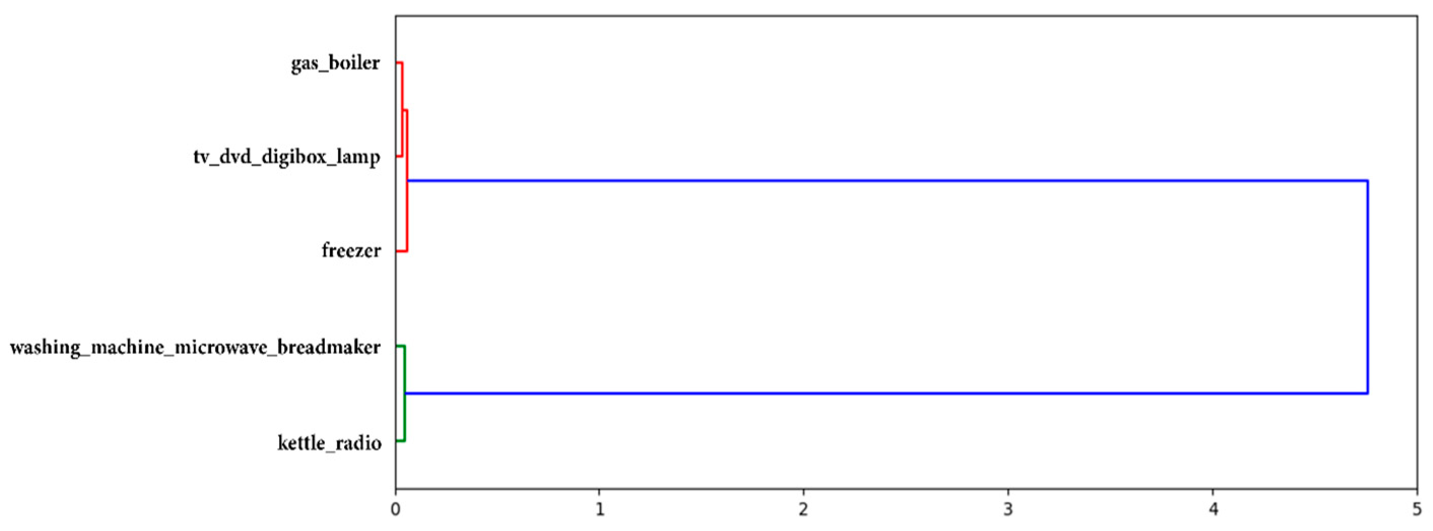
| Association Rule | Confidence | Hour | From (dd-mm-yy) | To (dd-mm-yy) |
|---|---|---|---|---|
| tv_dvd_digibox_lamp ⟹ gas_boiler | 100.0% | 0–24 | 9-3-2013 | 1-10-2013 |
| gas_boiler ⟹ tv_dvd_digibox_lamp | 100.0% | 0–24 | 9-3-2013 | 1-10-2013 |
| tv_dvd_digibox_lamp ⟹ freezer | 98–100% | 0–24 | 9-3-2013 | 1-10-2013 |
| freezer ⟹ tv_dvd_digibox_lamp | 99–100% | 0–24 | 9-3-2013 | 1-10-2013 |
| gas_boiler ⟹ freezer | 97–100% | 0–24 | 10-3-2013 | 1-10-2013 |
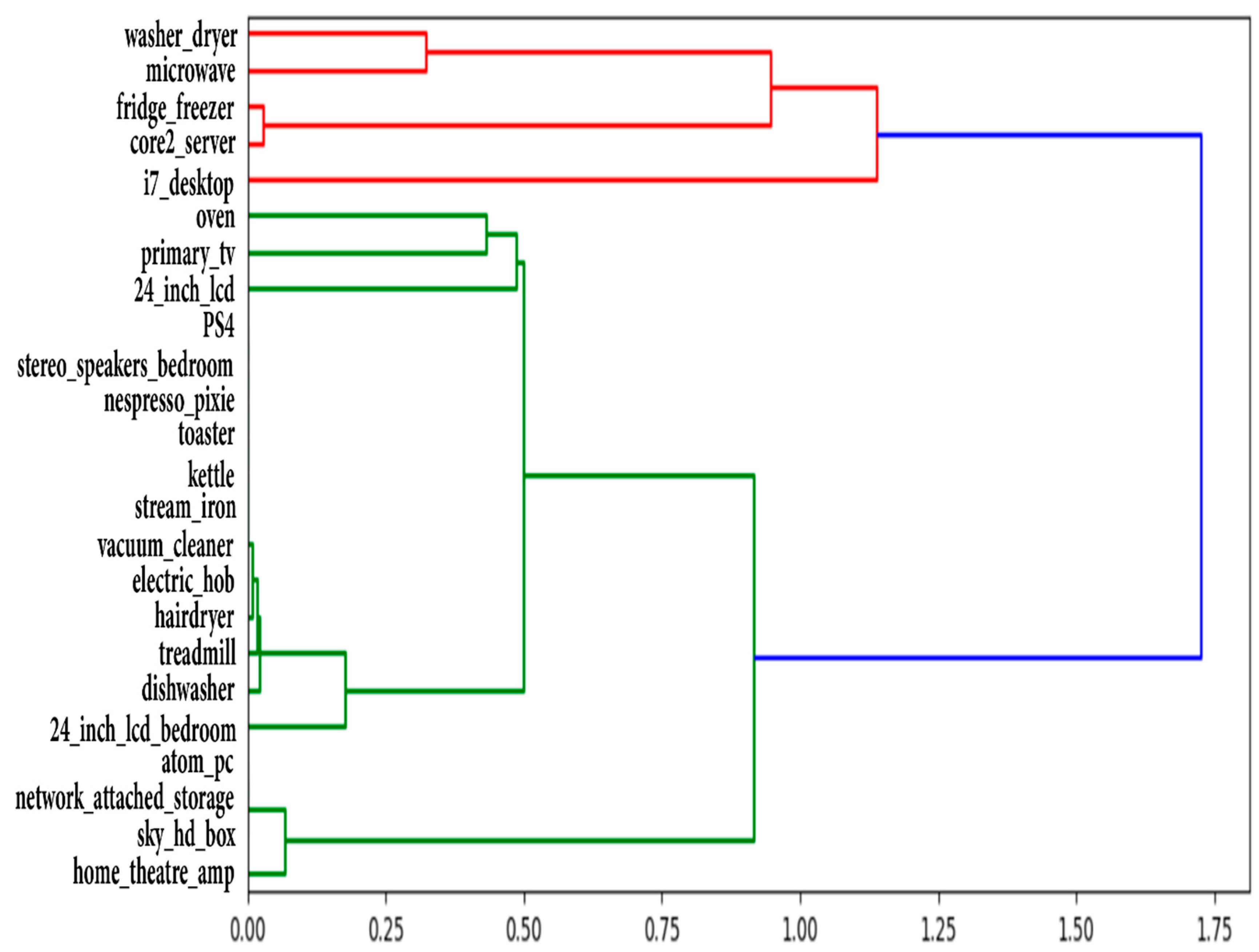
| Association Rule | Confidence | Hour | From (dd-mm-yy) | To (dd-mm-yy) |
|---|---|---|---|---|
| primary_tv ⟹ i7_desktop | 100% | 21 | 29-6-2014 | 11-11-2014 |
| primary_tv ⟹ i7_desktop | 99% | 22 | 29-6-2014 | 12-11-2014 |
| primary_tv ⟹ i7_desktop | 92% | 23 | 29-6-2014 | 12-11-2014 |
| 24_inch_lcd ⟹ i7_desktop | 100% | 11 | 30-6-2014 | 6-9-2014 |
| 24_inch_lcd ⟹ i7_desktop | 100% | 12 | 30-6-2014 | 7-9-2014 |
| 24_inch_lcd ⟹ i7_desktop | 100% | 13 | 30-6-2014 | 7-9-2014 |
| 24_inch_lcd ⟹ i7_desktop | 100% | 14 | 30-6-2014 | 7-9-2014 |
| 24_inch_lcd ⟹ i7_desktop | 100% | 15 | 30-6-2014 | 7-9-2014 |
| 24_inch_lcd ⟹ i7_desktop | 100% | 16 | 30-6-2014 | 6-9-2014 |
| 24_inch_lcd ⟹ i7_desktop | 100% | 17 | 30-6-2014 | 6-9-2014 |
| 24_inch_lcd ⟹ i7_desktop | 100% | 18 | 29-6-2014 | 6-9-2014 |
| 24_inch_lcd ⟹ i7_desktop | 100% | 19 | 29-6-2014 | 6-9-2014 |
| 24_inch_lcd ⟹ i7_desktop | 100% | 20 | 30-6-2014 | 6-9-2014 |
| oven ⟹ i7_desktop | 100% | 19 | 8-7-2014 | 13-11-2014 |
| oven ⟹ i7_desktop | 100% | 20 | 29-6-2014 | 10-11-2014 |
| oven ⟹ i7_desktop | 100% | 21 | 29-6-2014 | 11-11-2014 |
| oven ⟹ i7_desktop | 100% | 22 | 30-6-2014 | 12-11-2014 |
| oven ⟹ i7_desktop | 100% | 23 | 30-6-2014 | 12-11-2014 |
| Association Rules | Hierarchical Clustering | |
|---|---|---|
| Associations Discovered | Based on the behavior for each hour per day. | Based on the behavior across the 24 h. |
| Exhibition Period | Identifies the lifespan for the discovered associations. | Identifies the associations across all the recorded days. |
| History | Behavioral history can be obtained. | No history can be obtained. |
© 2019 by the authors. Licensee MDPI, Basel, Switzerland. This article is an open access article distributed under the terms and conditions of the Creative Commons Attribution (CC BY) license (http://creativecommons.org/licenses/by/4.0/).
Share and Cite
Osama, S.; Alfonse, M.; M. Salem, A.-B. Mining Temporal Patterns to Discover Inter-Appliance Associations Using Smart Meter Data. Big Data Cogn. Comput. 2019, 3, 20. https://doi.org/10.3390/bdcc3020020
Osama S, Alfonse M, M. Salem A-B. Mining Temporal Patterns to Discover Inter-Appliance Associations Using Smart Meter Data. Big Data and Cognitive Computing. 2019; 3(2):20. https://doi.org/10.3390/bdcc3020020
Chicago/Turabian StyleOsama, Sarah, Marco Alfonse, and Abdel-Badeeh M. Salem. 2019. "Mining Temporal Patterns to Discover Inter-Appliance Associations Using Smart Meter Data" Big Data and Cognitive Computing 3, no. 2: 20. https://doi.org/10.3390/bdcc3020020
APA StyleOsama, S., Alfonse, M., & M. Salem, A.-B. (2019). Mining Temporal Patterns to Discover Inter-Appliance Associations Using Smart Meter Data. Big Data and Cognitive Computing, 3(2), 20. https://doi.org/10.3390/bdcc3020020