Article

Lithology Identification from Well Logs via Meta-Information Tensors and Quality-Aware Weighting

1
School of Software, East China University of Technology, Nanchang 330013, China
2
Jiangxi Engineering Technology Research Center of Nuclear Geoscience Data Science and System, East China University of Technology, Nanchang 330013, China
3
School of Artificial Intelligence and Information Engineering, East China University of Technology, Nanchang 330013, China
*
Author to whom correspondence should be addressed.
Big Data Cogn. Comput. 2026, 10(2), 47; https://doi.org/10.3390/bdcc10020047
Submission received: 16 December 2025 / Revised: 17 January 2026 / Accepted: 26 January 2026 / Published: 2 February 2026

Abstract

In practical well-logging datasets, severe missing values, anomalous disturbances, and highly imbalanced lithology classes are pervasive. To address these challenges, this study proposes a well-logging lithology identification framework that combines Robust Feature Engineering (RFE) with quality-aware XGBoost. Instead of relying on interpolation-based data cleaning, RFE uses sentinel values and a meta-information tensor to explicitly encode patterns of missingness and anomalies, and incorporates sliding-window context to transform data defects into discriminative auxiliary features. In parallel, a quality-aware sample-weighting strategy is introduced that jointly accounts for formation boundary locations and label confidence, thereby mitigating training bias induced by long-tailed class distributions. Experiments on the FORCE 2020 lithology prediction dataset demonstrate that, relative to baseline models, the proposed method improves the weighted F1 score from 0.66 to 0.73, while Boundary F1 and the geological penalty score are also consistently enhanced. These results indicate that, compared with traditional workflows that rely solely on data cleaning, explicit modeling of data incompleteness provides more pronounced advantages in terms of robustness and engineering applicability.

1. Introduction

With the advancing development of unconventional oil and gas resources and deepwater offshore fields, relying solely on limited core and mud-logging data for lithology interpretation struggles to meet the dual requirements of high spatial resolution and real-time performance in reservoir characterization and wellbore engineering [1,2]. Consequently, leveraging machine learning to automatically identify lithology from well-logging curves has become a core auxiliary tool in exploration and production [3,4]. Recently, public competitions such as SEG 2016 [5,6] and FORCE 2020 [7,8,9] have released benchmark datasets containing well-log–lithology labels. These initiatives have established a standard research paradigm—using well logs as inputs for multi-class lithology prediction—and enabled fair, uniform evaluation of diverse methods [10].
From a methodological perspective, early studies predominantly employed traditional algorithms like Support Vector Machines (SVMs), Random Forests, and Gradient Boosting Trees, demonstrating the feasibility of workflows based on hand-crafted features [11,12]. With the rise in computing power and open-source tools, deep learning models—including 1D-CNN, LSTM, and Transformers—have been introduced to automatically extract features from logging sequences [13,14,15]. On experimental datasets with relatively complete features and homogeneous geological conditions, these end-to-end models often achieve significantly higher accuracy than traditional algorithms and effectively capture long-range dependencies associated with sedimentary rhythms [16]. However, their high sensitivity to data quality creates significant generalization bottlenecks when applied to noisy industrial datasets. More recently, sequence models that fuse convolutional and recurrent structures and foundation-model style pretraining for cross-well generalization have been explored [17]. To further address complex lithofacies identification under weaker geological priors, recent studies have explored various advanced techniques. For instance, ref. [18] proposed a partial domain adaptation method to handle domain shifts, while ref. [19] utilized wavelet transforms and adversarial learning for cross-well identification. Others have investigated semi-supervised networks [20] and deep kernel methods [21] to enhance feature extraction effectiveness.
Data quality issues are particularly acute in large-scale real-world datasets like FORCE 2020 [7,8,9]. First, well-logging curves exhibit severe non-random missing values and tool-related anomalies, both between and within wells [22,23,24]. Second, lithology classes follow a typical long-tailed distribution, where samples for specific lithofacies are extremely scarce [25,26]. Analyses of competition results indicate that even with sophisticated feature engineering and model tuning, state-of-the-art solutions achieve only ~80% accuracy on blind-test wells, with substantial misclassification of rare lithologies such as coal and tuff [27,28]. Existing workflows typically follow a “cleaning-then-modeling” pipeline, filling missing data via interpolation. While this satisfies input completeness requirements, it effectively smoothes out missing patterns and anomalous responses, ignoring critical information related to borehole collapse, wellbore conditions, and formation heterogeneity encoded within these “defects” [29,30,31].
To address missing data, recent studies have proposed log-reconstruction frameworks based on Transformers [32] or generative adversarial networks (GANs [33]) to recover missing curves at the sequence level. While numerically reduce the missing rate, they still treat “missingness” purely as noise to be repaired, rather than as a feature signal for downstream classification. Regarding class imbalance [34], techniques like undersampling, SMOTE [35], and weighted loss functions (e.g., focal loss [36]) are widely used. However, most methods adjust loss primarily based on class frequency, insufficiently accounting for the importance of formation boundaries and label confidence. Consequently, the training objective often deviates from the actual risk structure encountered in geological interpretation.
It is crucial to distinguish the proposed data quality modeling approach from these prevalent strategies. Conceptually, unlike reconstruction-based methods (e.g., interpolation or autoencoders) that attempt to “guess” missing values—potentially introducing smoothing artifacts or false geological signals—our framework treats “missingness” itself as an informative feature. Practically, unlike implicit mask-based strategies used in deep learning (e.g., Transformers which require massive data to learn attention weights), our approach explicitly aggregates missing patterns into statistical meta-features. This allows tree-based models to directly utilize data quality signals as decision rules (e.g., “If RHOB is missing, rely on GR”) without the need for black-box attention mechanisms.
Furthermore, the design of evaluation protocols directly impacts model applicability [37,38,39]. Many studies rely on random sample-wise splits or standard K-fold cross-validation, ignoring the inherent spatial autocorrelation of logging data [40,41]. Including samples from the same well in both training and test sets allows models to “memorize” well-specific patterns, leading to data leakage and overestimated generalization capabilities. Essentially, this approach resembles “intra-well interpolation” rather than true “cross-well prediction.” Therefore, for practical applications, a strict well-based splitting scheme (e.g., GroupKFold) must be considered a fundamental constraint in experimental design [42,43].
In view of these challenges, this study approaches the problem through data quality modeling. We revisit the strengths of tree-based models on tabular data to construct a robust lithology identification framework tailored to noisy, incomplete logging data. The high-level motivation of our approach rests on two key insights addressing the aforementioned difficulties. First, regarding non-random missing data, we argue that missing patterns often carry specific physical significance (e.g., bad borehole conditions) rather than being random noise. Therefore, instead of obscuring these patterns via interpolation, we employ Unified Sentinel Encoding to explicitly preserve them as learnable features. Second, to address the long-tailed distribution where minority lithologies are often overwhelmed, we introduce a Quality-Aware Weighting mechanism. This strategy dynamically prioritizes high-quality samples within rare classes, ensuring the model effectively learns from the “tail” without being dominated by the “head” classes. The main contributions are:
(1)
A Robust Feature Engineering (RFE) framework
By explicitly modeling missingness and anomaly patterns through meta-information encoding, we transform data quality information—traditionally treated as noise—into auxiliary discriminative features, eliminating dependence on complex imputation.
(2)
A quality-aware XGBoost classification model
We design a multi-factor sample-weighting strategy integrating class balance, boundary neighborhoods, and label confidence. Additionally, we introduce a comprehensive evaluation system incorporating Boundary F1 and Penalty Scores, significantly enhancing the characterization of rare lithologies and formation boundaries.
(3)
Systematic robustness evaluation
Using a strict cross-well validation protocol (GroupKFold) on the FORCE 2020 [7,8,9] dataset, experiments demonstrate that the proposed method significantly outperforms the conventional “interpolation + modeling” paradigm, particularly on incomplete data and challenging wells.
The remainder of this paper is organized as follows: Section 2 details the proposed Robust Feature Engineering (RFE) framework and the quality-aware weighting strategy. Section 3 presents the experimental results on the FORCE 2020 [7,8,9] dataset, demonstrating the performance of the proposed method. Section 4 provides a comprehensive discussion on the findings, geological interpretability, and limitations. Finally, Section 5 concludes the study and outlines future research directions.

2. Materials and Methods

2.1. Dataset and Data Analysis

This study utilizes the public dataset from the FORCE 2020 [7,8,9] Lithology Prediction Challenge. Comprising data from 118 wells in the Norwegian sector of the North Sea, the dataset provides a suite of conventional logging curves (e.g., GR, RHOB, NPHI) aligned with corresponding lithology labels. The geographic distribution of the wells is shown in Figure 1.
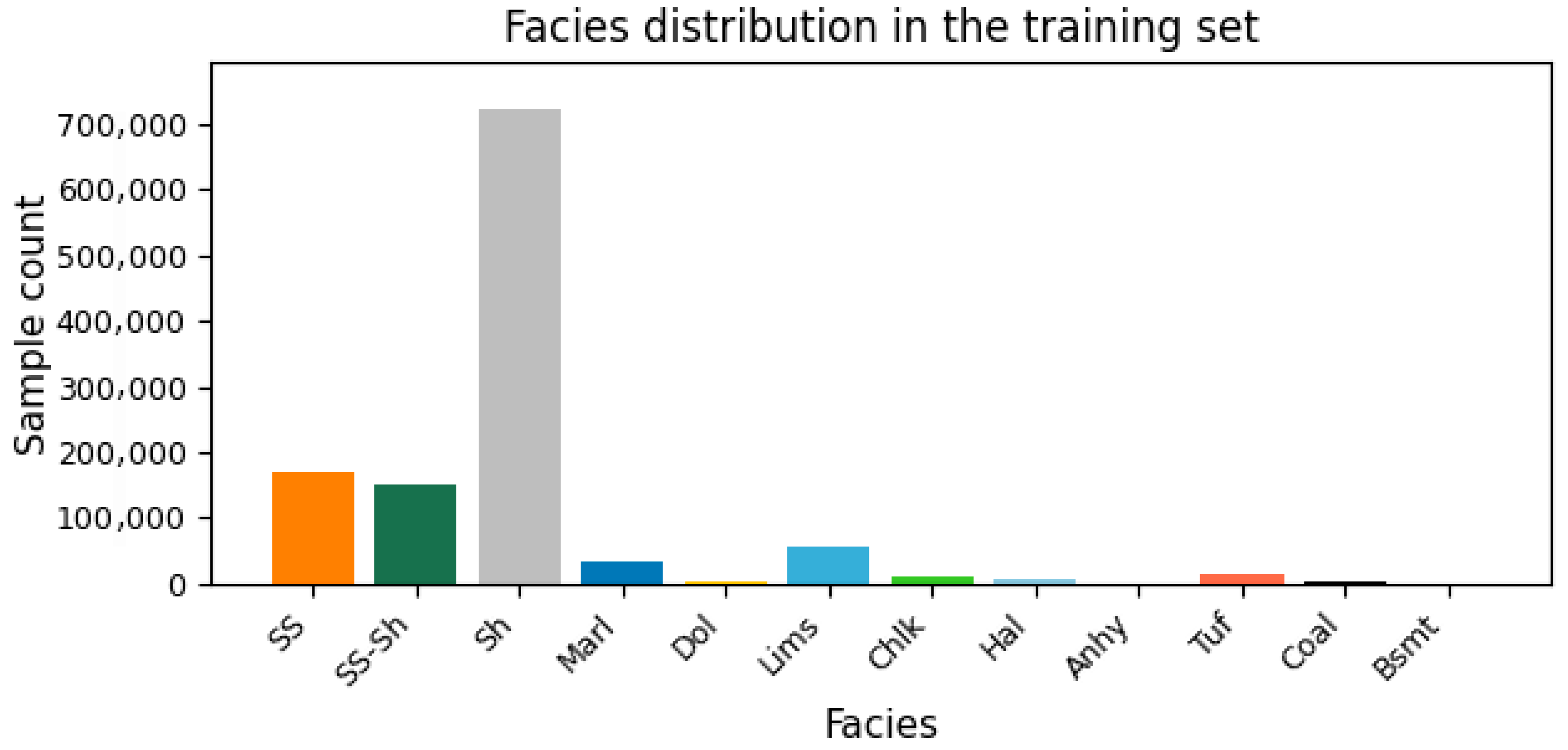
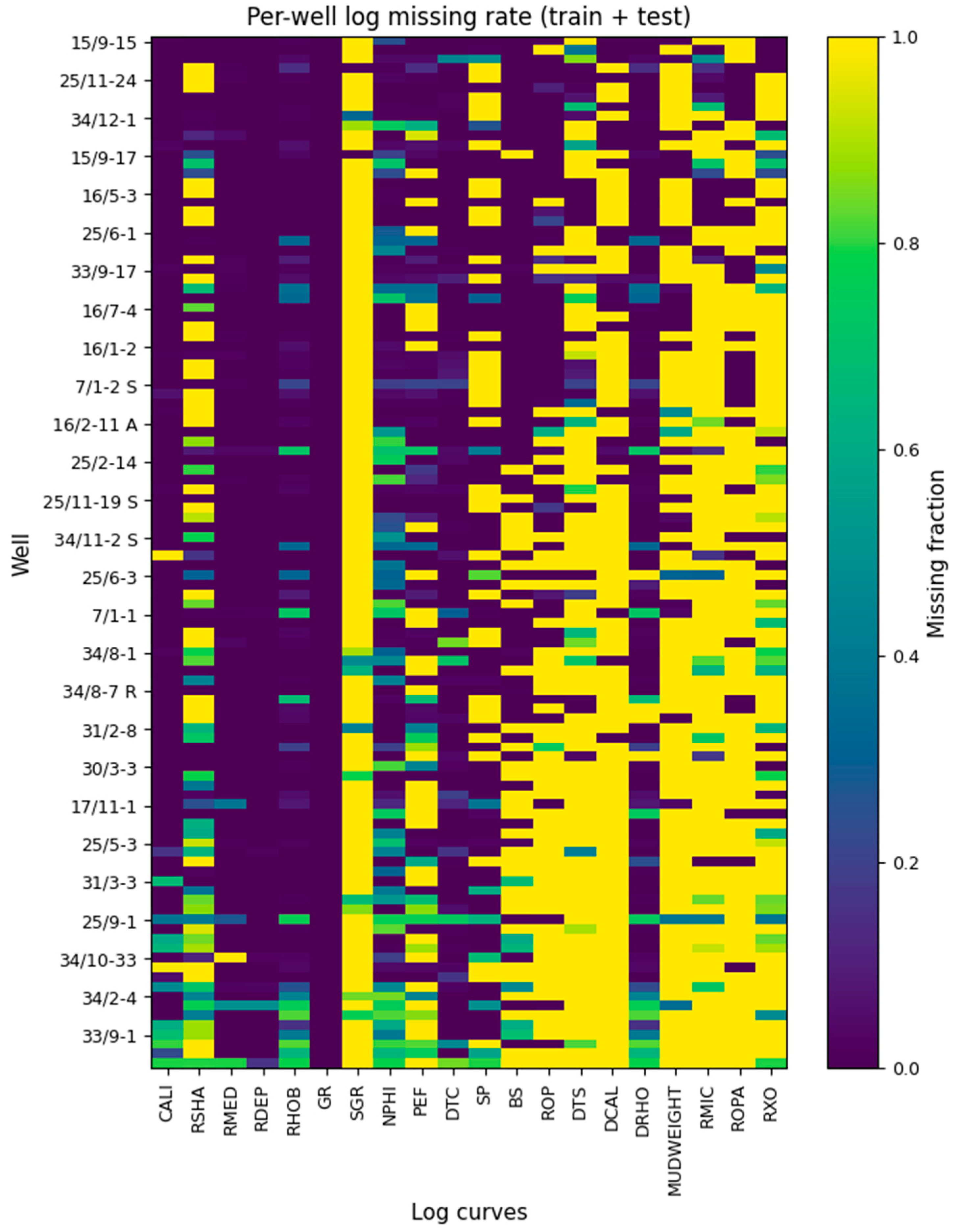
However, for practical modeling, this dataset presents two significant challenges. First, there is extreme class imbalance (Figure 2). Second, the data suffers from severe non-random missingness (Figure 3). Naive interpolation-based imputation risks masking the underlying geological indicators encoded within these missing patterns. And, the lithology classification and corresponding visualization colors used in this study are presented in Table 1.

2.2. Robust Feature Engineering (RFE) Framework

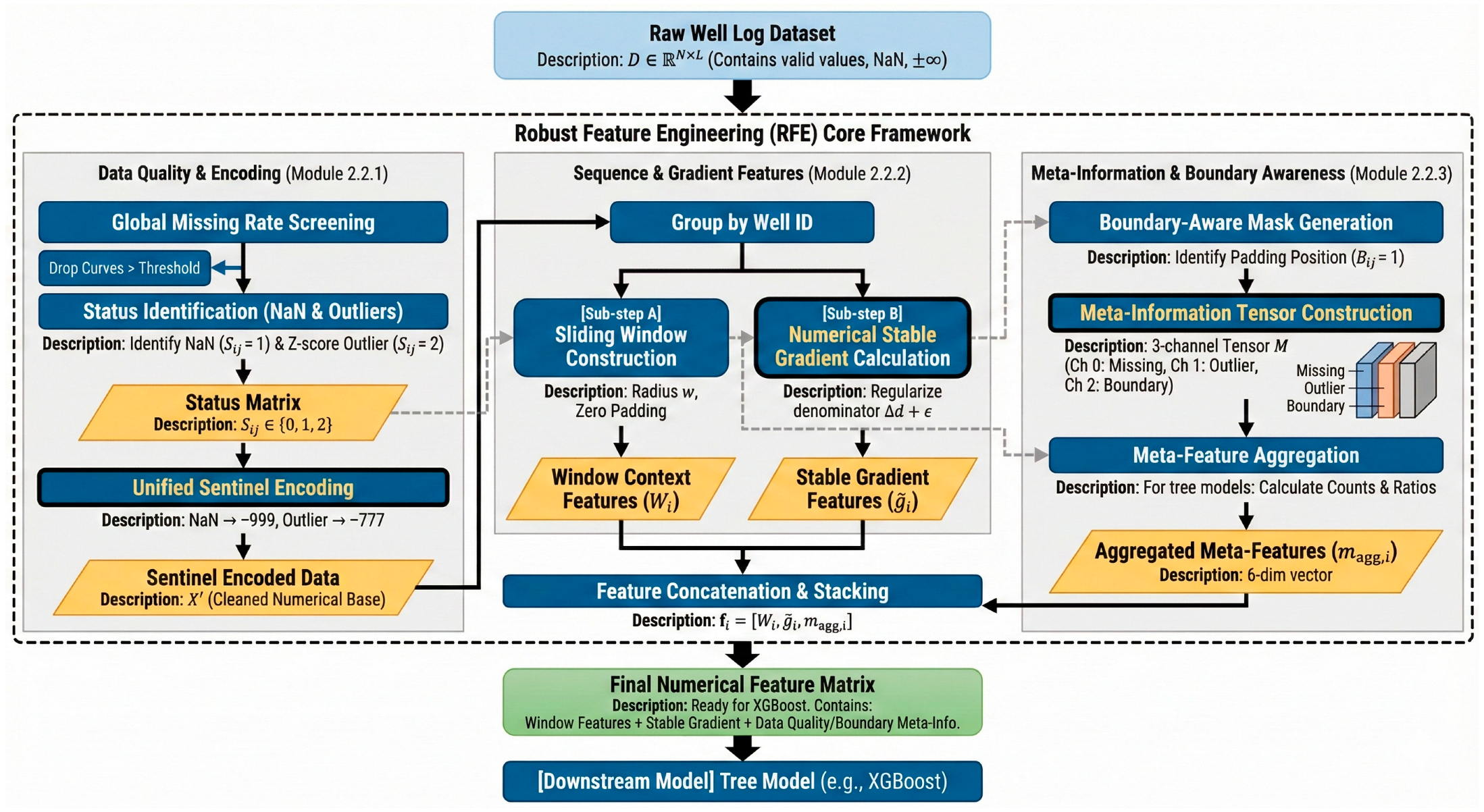
To address these challenges, this study developed a Robust Feature Engineering (RFE) framework [44,45,46]. Unlike deep neural networks, RFE fully exploits the intrinsic properties of tree models to directly address incomplete tabular data. The workflow is illustrated in Figure 4.

2.2.1. Global Missing-Rate Filtering and Unified Sentinel Encoding

To avoid introducing artificial noise through interpolation, we first assess the missing rate of each logging curve globally. Curves exceeding a threshold (e.g., 90%) are removed. For the retained curves, RFE constructs a status matrix based on training set statistics [47]. For an arbitrary logging measurement X t , l at depth t   and curve l :
s t , l = 1 , i f   X t , l   i s   o r i g i n a l l y   m i s s i n g   ( N a N o r ± ) 2 , i f   X t , l   i s   a n u m e r i c a l   o u t l i e r   ( | z t , l | > T z ) 0 , o t h e r w i s e   ( v a l i d m e a s u r e m e n t ) ,
where T z   denotes the anomaly detection threshold (set to 5) [26]. We set the anomaly threshold to T z   = 5 rather than the standard 3 σ . This stricter threshold is chosen because well-logging data naturally exhibits high geological variability; a lower threshold would incorrectly flag legitimate geological anomalies (such as thin coal beds or gas-bearing layers) as sensor errors. Subsequently, we map these non-standard states to fixed sentinel values (e.g., −999 for missing, −777 for anomalies), empowering tree models to segregate these samples during node splitting. We employ the industry-standard value of −999 (LAS format convention) to denote missing data. It is worth noting that tree-based models are largely insensitive to the specific magnitude of these sentinel values, provided they fall strictly outside the valid physical range. Unlike neural networks which are sensitive to input scaling, decision trees rely on rank-based splitting. The model autonomously learns a threshold (e.g., Feature < −500) to isolate missing samples, ensuring that the classification performance remains robust to the specific choice of the sentinel scheme (e.g., −999 vs. −777), as verified by our internal sensitivity checks.

2.2.2. Sliding-Window Context Features and Numerically Stable Gradients

Considering stratigraphic continuity, we construct a sliding window of radius k centered at depth index t to extract a context feature vector   w t   [48,49,50]:
w t = [ x t k , , x t 1 , x t , x t + 1 , , x t + k ] R ( 2 k + 1 ) L ,
where x t R L denotes the L-dimensional logging measurement vector. Additionally, to capture abrupt changes near boundaries, we compute the first-order gradient. To address repeated depth records ( Δ D e p t h = 0 ), we introduce a regularization term ε d :
G r a d l s t a b ( t ) = X t , l X t 1 , l Δ D e p t h t + ε d   ,
where ε d   is a small positive constant to avoid division-by-zero errors.

2.2.3. Boundary-Aware Mask and Meta-Information Tensor

The use of sliding windows introduces padding at sequence ends. RFE exploits this to derive a boundary-indicator vector   b t { 0 , 1 } . We unify the states of missingness, outliers, and padding into a Meta-Information Tensor M m e t a { 0 , 1 } N × L × 3 . The three channels are defined as:
M m e t a ( t , l , 0 ) = I ( s t , l = 1 )   ( M i s s i n g ) ,
M m e t a ( t , l , 1 ) = I ( s t , l = 2 )   ( O u t l i e r ) ,
M m e t a ( t , l , 2 ) = b t °   ( B o u n d a r y P a d d i n g )
To explicitly quantify the data quality at each depth t , we aggregate the meta-information tensor across all logging curves. The count-based meta-features ( m m i s s , m o u t ) and ratio-based meta-features ( r m i s s , r o u t ) are mathematically derived as follows:
m m i s s t = l = 1 L M m e t a t , l , 0 , m o u t ( t ) = l = 1 L M m e t a ( t , l , 1 )   r m i s s t = m m i s s t L , r o u t ( t ) = m o u t ( t ) L
where L is the total number of logging curves, and M m e t a ( t , l , c )   denotes the element of the tensor at depth t , curve   l , and channel   c . These features serve as explicit indicators of local data completeness and reliability.
For tree models, M m e t a is aggregated into count-type and ratio-type meta-features. By concatenating these with window features and gradients, we obtain the final input feature vector f t :
f t = w t , G r a d s t a b ( t ) , m t m i s s , m t o u t , b t , r t m i s s , r t o u t , r t b n d
This joint modeling enhances sensitivity to thin beds and formation boundaries [48,50].

2.3. Quality-Aware XGBoost Model

We adopt XGBoost as the core classifier, employing a quality-aware sample-weighting strategy [51,52]. The training weight w t for the t-th sample is defined as the product of three factors:
w t = w c l a s s ( y t ) w b o u n d a r y ( t ) w c o n f ( t )
where
1.
w c l a s s ( y t ) : Inverse to class frequency, balancing rare lithologies:
w c l a s s ( y t ) = N t o t a l C N y t
N t o t a l is the total number of training samples, C = 12 is the number of lithology classes, and   N y t is the frequency of class   y t   in the training set.
2.
w b o u n d a r y ( t ) : To enhance the model’s sensitivity to lithological transitions, we assign higher penalties to boundary samples [53]:
w b o u n d a r y ( t ) = 1.2 , i f   j [ t 1 , t + 1 ] , y j y t 0.7 , o t h e r w i s e
This strategy up-weights the transition zones (window radius r = 1 ) where misclassification is geologically costly.
3.
w c o n f ( t ) : To suppress noise from poor-quality logs, we down-weight samples from wells with severe data loss. Let ρ w e l l be the global missing rate of a well. The confidence weight is defined as:
w c o n f ( t ) = 0.7 , i f   ρ w e l l > 0.6 1.0 , o t h e r w i s e
The threshold τ m i s s = 0.6 and the penalty factor 0.7 are empirically selected to reduce the impact of feature-deficient wells while retaining usable information.

2.4. Experimental Setup and Evaluation Metrics

Cross-Validation Strategy: We employ a 10-fold well-wise grouped cross-validation (GroupKFold), where the WELL identifier serves as the grouping label to preventing sample leakage [54].
Evaluation Metrics We employ a multi-dimensional evaluation framework:
  • Weighted F1-Score: To account for class imbalance, we adopt the Weighted F1-Score;
  • Boundary F1 Score: Evaluates performance strictly on a boundary sample set B , defined as indices within radius r of a transition
    B = { i | k [ i r , i + r ] , y k y k + 1 }
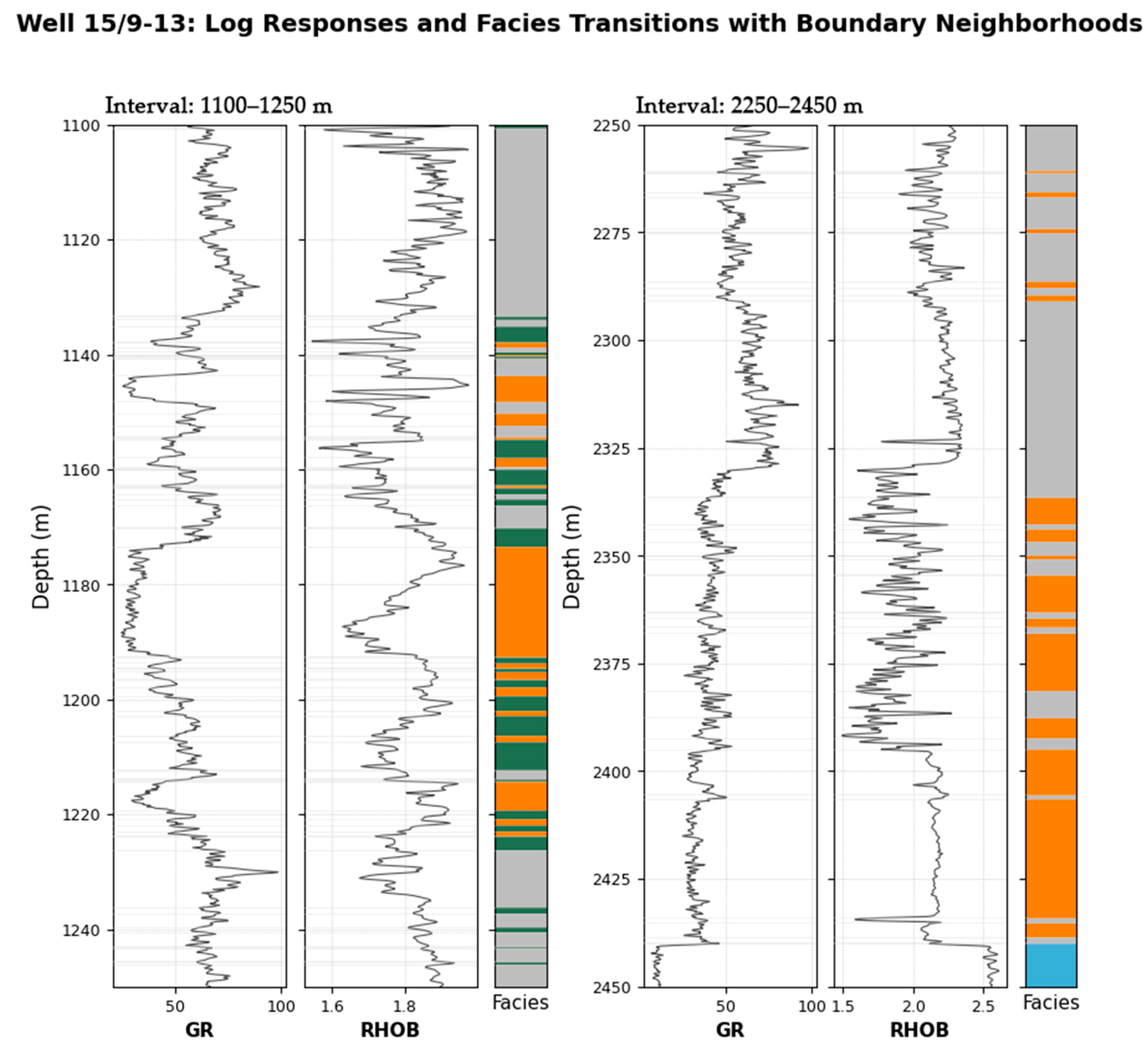
This filters out easy samples in thick, homogeneous layers, as illustrated in Figure 5;
3.
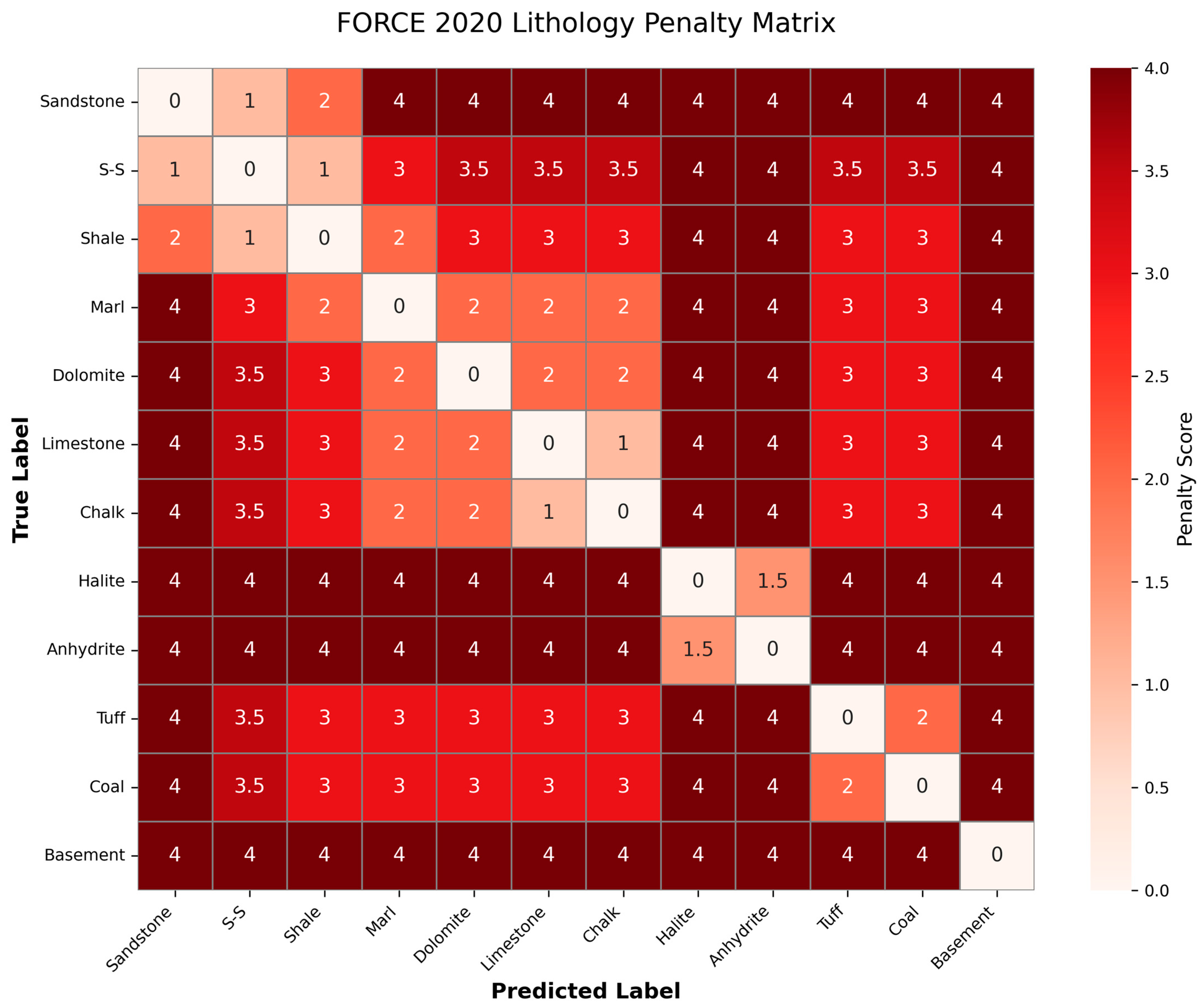
Geological Penalty Score: To assess geological plausibility, we adopt the lithology Penalty Matrix   A   defined in the FORCE 2020 competition (see Figure 6) [52]. This matrix assigns misclassification costs based on petrophysical similarity and engineering risk.
The normalized Geological Penalty Score is defined as:
S = 1 N i = 1 N A y i , y ¯ i
A value of   S   closer to 0 indicates lower engineering risk.

3. Results

3.1. Baseline Comparison and Ablation Study

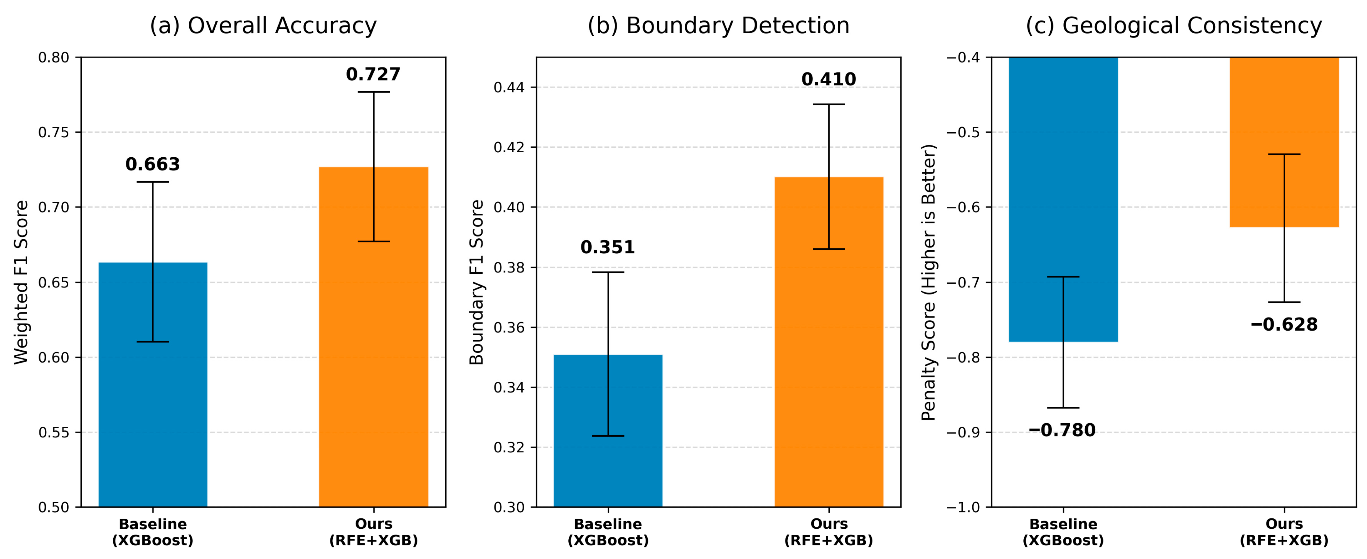
We first evaluated the impact of the proposed RFE framework by comparing it against the Standard XGBoost Baseline. To ensure a fair comparison regarding data completeness, the baseline utilizes XGBoost’s native sparsity-aware split finding algorithm to handle missing values automatically without external imputation. The evaluation was conducted using a 10-fold GroupKFold validation. We specifically chose GroupKFold (grouped by Well ID) over standard random sample-wise splitting to avoid data leakage. Due to the high spatial autocorrelation of well-log curves, random splitting would place adjacent, highly correlated samples into both training and testing sets, effectively reducing the task to “intra-well interpolation.” While this would yield overly optimistic performance metrics (likely inflating accuracy to >95%), it fails to reflect the model’s generalization ability to undrilled blind wells. Therefore, strict well-based splitting is essential for a realistic evaluation of geological applicability. As illustrated in Figure 7, the proposed method achieved improvements across all three metrics. Specifically:
Overall Accuracy: The Weighted F1 score increased significantly from 0.664 (Baseline) to 0.727 (RFE + XGBoost).
Boundary Detection: The Boundary F1 score surpassed the 0.40 threshold, reaching 0.410 compared to 0.351 for the baseline.
Geological Consistency: The Penalty Score improved from −0.780 to −0.628, indicating a marked reduction in high-penalty misclassifications.
To strictly isolate component contributions, we conducted a comprehensive ablation study (Table 2). Results show that while the Baseline yields a Weighted F1 of 0.6635 (Penalty: −0.7804), the Feature Engineering (FE) module specifically boosts F1 to 0.7259, and the Weighting strategy independently optimizes the Penalty Score to −0.6346 for geological risk control. Integrating both, the final RFE + XGBoost framework achieves superior performance across all metrics (F1: 0.7272, Penalty: −0.6289), with paired t-tests confirming statistically significant improvements over the baseline (p < 0.01 for both weighted F1 and penalty scores).
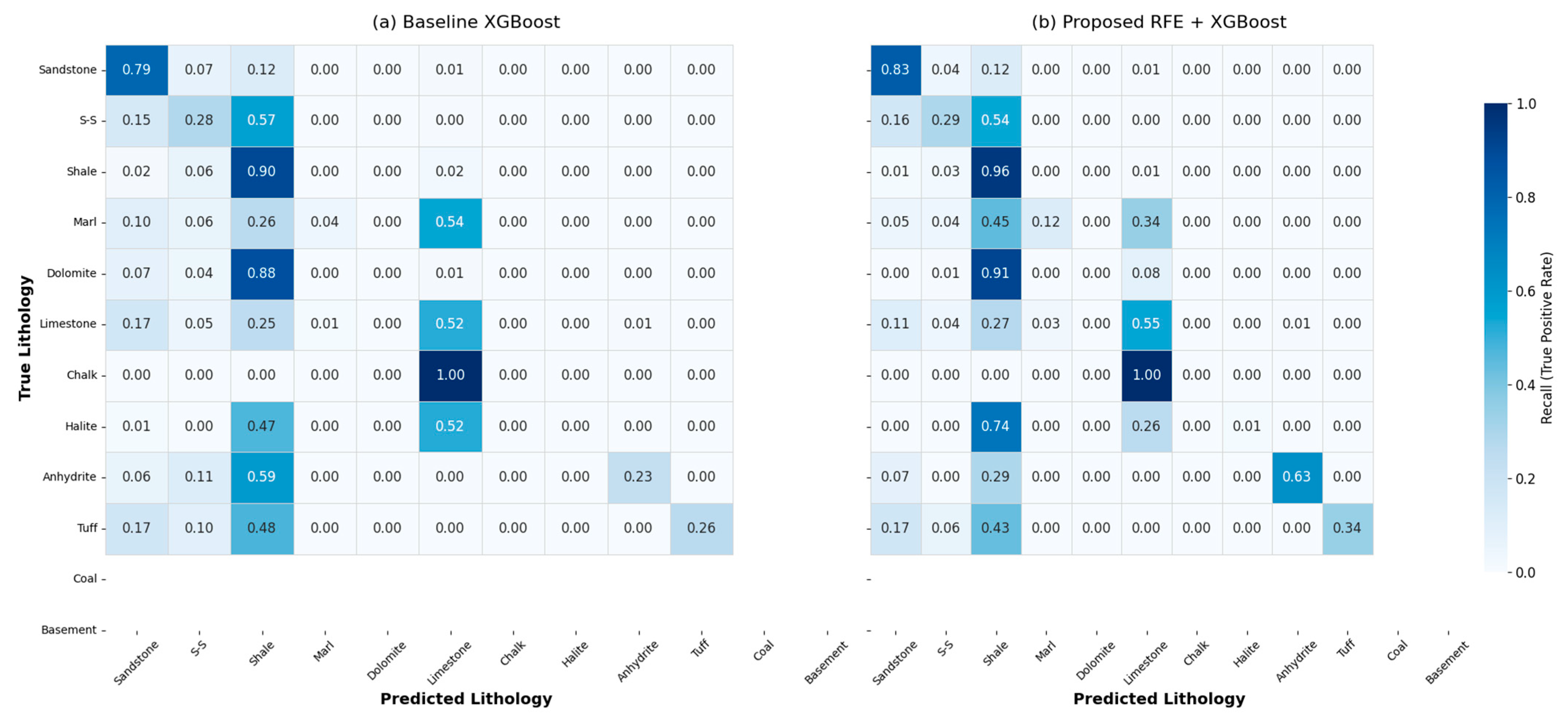
To dissect the model’s discriminative capabilities across varying lithologies, we compared the row-normalized confusion matrices on the independent test set (Figure 8). In the baseline model (Figure 8a), the recall for rare lithologies such as Anhydrite and Tuff was notably poor (0.23 and 0.26, respectively). With the RFE framework (Figure 8b), the recall for Anhydrite surged to 0.63, and Tuff improved to 0.34. Additionally, the recall for the majority class (Shale) further improved from 0.90 to 0.96.

3.2. Robustness Analysis Under Varying Data Completeness

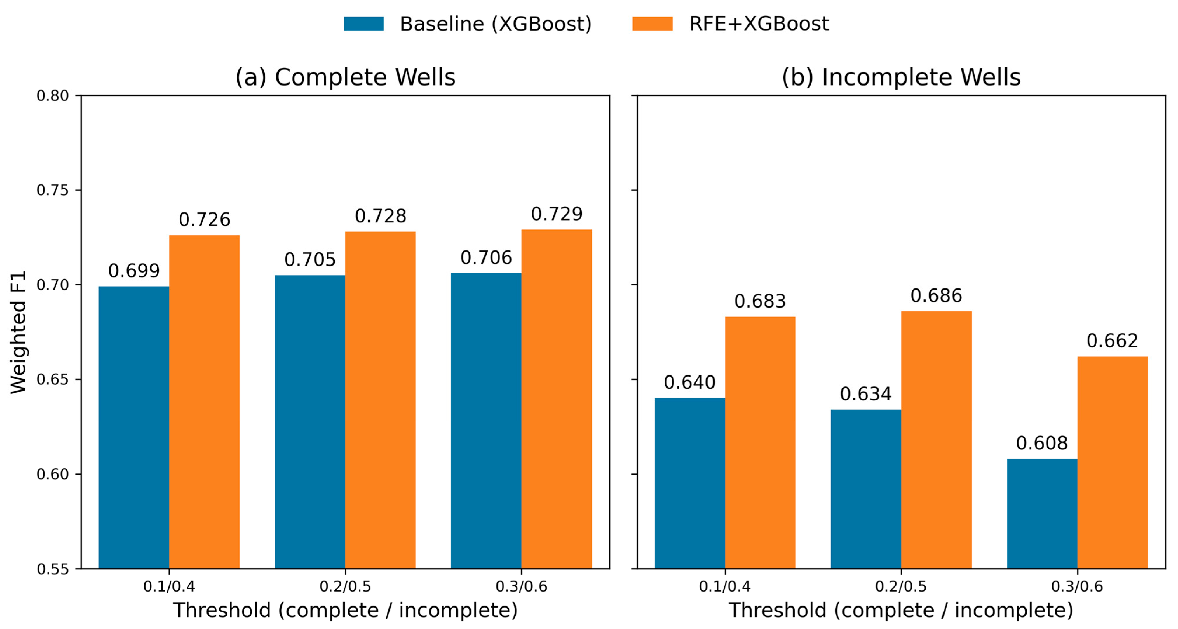
To investigate model stability, we stratified the test wells into “Feature-Complete” and “Feature-Deficient” groups based on missing rate thresholds (see Table 3 and Figure 9).
In feature-complete wells: The RFE + XGBoost model maintained a Weighted F1 score between 0.726 and 0.729, consistently outperforming the baseline (0.699–0.706).
In feature-deficient wells: As the selection criteria became stricter (isolating wells with higher missing rates), the baseline model suffered a precipitous decline in performance (from 0.640 down to 0.608). In contrast, the RFE-based model demonstrated exceptional resilience, maintaining a score of 0.662 even under the most challenging conditions (Threshold 0.3/0.6).
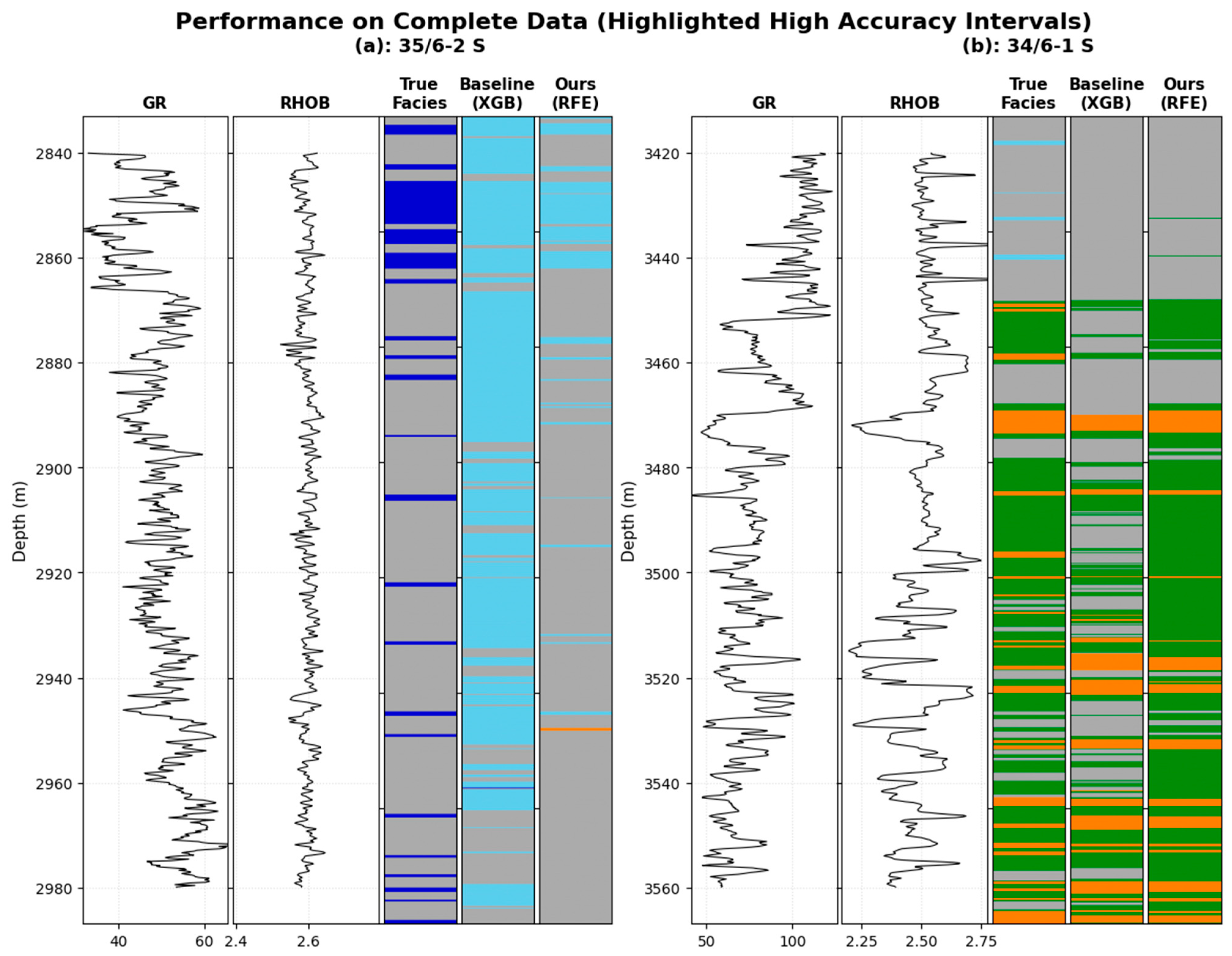
To visualize this robustness, we present comparative case studies. Figure 10 displays the results for feature-complete wells (e.g., Well 35/6-2 S). While both models capture primary trends, the RFE model produces a smoother lithology profile with sharper boundaries, effectively suppressing high-frequency noise.
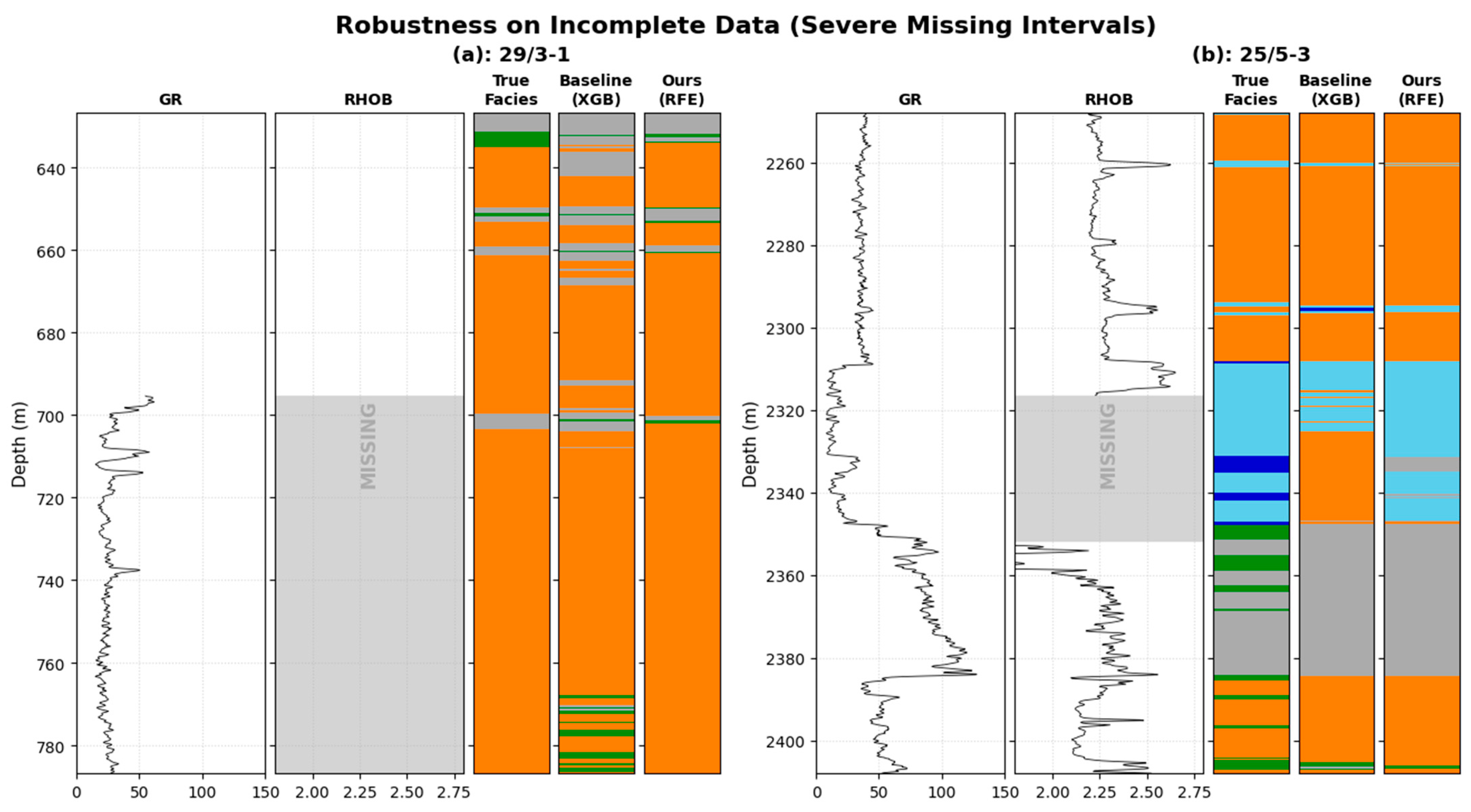
Figure 11 illustrates the performance on feature-deficient wells (e.g., Well 29/3-1). In intervals where the RHOB curve is missing (indicated by gray shading), the baseline model failed catastrophically, generating spurious reservoir indications (false positives). The RFE-based model, however, robustly identified these intervals as background formations, aligning with the ground truth.

3.3. Applicability on Different Tree Models

We extended the evaluation to Random Forest and LightGBM to verify the generalizability of the RFE framework. As detailed in Table 4, all three models exhibited substantial gains in both Weighted F1 and Boundary F1 scores when equipped with RFE features.
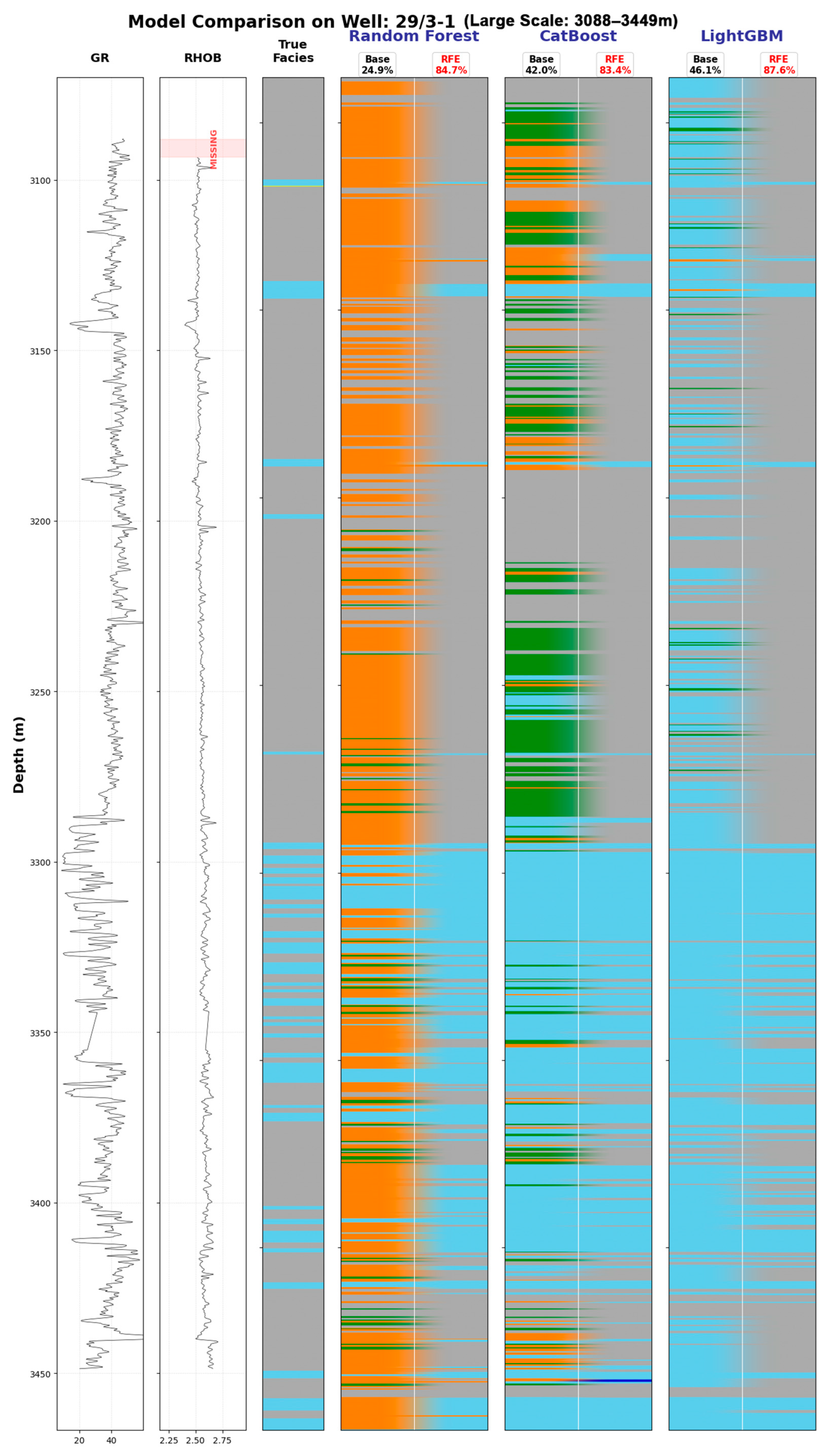
Visualizations in Figure 12 confirm that RFE effectively suppresses high-frequency noise across all tested models (Random Forest, CatBoost, and LightGBM), proving that the framework consistently guides tree-based models to focus on robust geological patterns.

4. Discussion

4.1. Mechanism Analysis: Why RFE Suits Tree Models Better than Interpolation

Traditional workflows typically treat missing values as noise to be repaired via interpolation [55,56]. However, our experimental results (Table 4, Figure 12) demonstrate that explicitly encoding missingness (RFE) consistently outperforms these methods across XGBoost, Random Forest, and LightGBM. The superiority of the RFE framework stems from the inherent inductive bias of tree-based models [57,58]. Unlike deep neural networks (e.g., CNNs, Transformers) which operate in continuous, differentiable function spaces and assume smoothness in the input manifold, tree models rely on hard threshold-based splitting [59]. While state-of-the-art Transformer-based architectures utilize attention masking to handle missing tokens, they typically require massive datasets to converge and lack the interpretability of decision trees in tabular geological settings. Deep learning models are highly sensitive to feature magnitude; feeding sentinel values like −999 directly would disrupt Batch Normalization statistics and induce gradient issues. In contrast, decision trees are invariant to monotonic transformations. They treat sentinel values merely as distinct states at the extreme end of the numerical axis. By learning a simple split threshold (e.g., Feature < −900), the model effectively isolates low-quality data into specific leaf nodes. The RFE framework leverages this property to reformulate the imputation challenge into a discrete state-classification problem, thereby transforming “missingness” from a disruptive noise into an informative feature signal.

4.2. Geological Consistency and Engineering Safety

From an engineering perspective, the improvement in Geological Penalty Score (from −0.780 to −0.628) is more significant than raw accuracy gains. This metric reflects a reduction in “non-geological errors,” such as confusing lithologies from fundamentally different depositional environments [60]. Specifically, the improvement in Anhydrite identification illustrates this mechanism. Anhydrite (high density, high resistivity) is often misclassified when the RHOB curve is missing. However, our framework explicitly flags the “Missing RHOB” state, forcing the model to shift attention to secondary diagnostic curves (e.g., PEF), thereby correctly retrieving the Anhydrite signature. The analysis of feature-deficient wells (Figure 11) highlights the safety implications of our approach. When valid input features (e.g., RHOB) are missing, the baseline model tends to generate spurious reservoir indications (false positives), effectively “hallucinating” oil/gas-bearing layers10. The RFE-XGBoost model, modulated by the quality-aware weighting strategy, successfully identifies these intervals as background formations. By suppressing high-frequency noise and avoiding erratic fluctuations in missing intervals, the proposed method maintains high operational reliability, which is critical for decision-making in undrilled blind wells [17].

4.3. Boundary Delineation Capabilities

The integration of sliding-window context and gradient features addresses the “point-wise” limitation of standard machine learning models [61]. The significant rise in Boundary F1 score (Figure 7b) confirms that the model has learned to attend to local stratigraphic dependence rather than fitting isolated logging values. This suggests that RFE effectively mitigates the shoulder-bed effect caused by limited tool resolution, enabling sharper delineation of thin interbeds and transition zones [62].

4.4. Limitations and Future Directions

Beyond robustness, computational efficiency is a critical factor for industrial deployment. The proposed feature engineering involves only linear-time window aggregations with a time complexity of O ( N ) , where N is the log depth. Unlike deep neural networks that require computationally intensive matrix operations and GPU acceleration, our framework is lightweight. On a standard CPU (Intel Core i7), the inference time for a complete well (approx. 10,000 sampling points) operates at a millisecond-level latency (typically <50 ms). This high efficiency makes the RFE-XGBoost framework ideal for real-time interpretation in edge computing scenarios, such as logging-while-drilling (LWD) environments.However, despite the robustness demonstrated, this work relies primarily on data-driven statistical encoding and has not fully exploited prior knowledge from rock physics [60,63]. Future research could integrate physical constraints (e.g., density and sonic bounds) directly into the loss function to further enhance interpretability. A practical implementation would involve adding a physics-guided regularization term ( L p h y ) to the loss function, penalizing predictions where the probabilistic output violates known rock-physics bounds (e.g., prohibiting high-porosity Sandstone predictions in high-density zones). Additionally, while RFE is tailored for tree models, investigating methods to embed similar meta-information mechanisms into deep sequence networks (e.g., via attention masking) remains a promising avenue for capturing longer-range sedimentary rhythms [17]. Finally, applying adversarial domain adaptation to transfer these missingness-handling capabilities to new fields with scarce labeled data addresses a critical need for industrial deployment [28].

5. Conclusions

This study proposed a Robust Feature Engineering (RFE) framework to address the challenges of non-random missing data and long-tailed class distributions in well-logging lithology identification. By replacing traditional interpolation with a unified sentinel encoding and meta-information tensor, we explicitly transformed data quality patterns into learnable features.
Experimental results on the FORCE 2020 [7,8,9] dataset demonstrate that the RFE-enhanced XGBoost model significantly outperforms the standard baseline. The proposed method not only improves overall classification accuracy (Weighted F1) but also enhances the delineation of formation boundaries (Boundary F1) and reduces geologically implausible errors (Penalty Score). Notably, in stress tests on feature-deficient wells, the method exhibited strong engineering resilience, preventing the performance collapse typically observed in models relying on data imputation.
Furthermore, comparative experiments confirmed that this meta-information encoding strategy provides universal performance gains across various tree-based models, including Random Forest, CatBoost, and LightGBM. These findings suggest that explicit modeling of data incompleteness offers a more robust and effective paradigm for industrial well-log analysis than traditional cleaning-then-modeling workflows.

Author Contributions

Conceptualization, G.Z.; methodology, W.C., G.Z. and F.D.; software, W.C. and F.D.; validation, P.D. and J.H.; writing—original draft preparation, W.C.; writing—review and editing, F.D. and P.D.; supervision, G.Z. and J.H.; funding acquisition, J.H. and G.Z. All authors have read and agreed to the published version of the manuscript.

Funding

This research was funded by the National Key Laboratory of Uranium Resources Exploration–Mining and Nuclear Remote Sensing, East China University of Technology (Grant No. 2024QZ-TD-10), under the project “Prospecting Information Extraction and Intelligent Mineralization Prediction for Sandstone-Type Uranium Deposits in the Southern Songliao Basin”, and by the Jiangxi Provincial Natural Science Foundation (Grant No. 20253BAC260013). The APC was funded by the above funders (Grant Nos. 2024QZ-TD-10 and 20253BAC260013).

Institutional Review Board Statement

Not applicable.

Informed Consent Statement

Not applicable.

Data Availability Statement

The data presented in this study are openly available in Zenodo at 10.5281/zenodo.4351155. The source code and the implementation of the proposed framework are openly available at: https://github.com/ccccwx/yanxingshibie/tree/main (accessed on 25 January 2026).

Conflicts of Interest

The authors declare no conflicts of interest.

References

  1. Wood, D.A. Extracting Useful Information from Sparsely Logged Wellbores for Improved Rock Typing of Heterogeneous Reservoir Characterization Using Well-Log Attributes, Feature Influence and Optimization. Pet. Sci. 2025, 22, 2307–2311. [Google Scholar] [CrossRef]
  2. Wang, L.; Fan, Y. Fast Inversion of Logging-While-Drilling Azimuthal Resistivity Measurements for Geosteering and Formation Evaluation. J. Pet. Sci. Eng. 2019, 176, 342–351. [Google Scholar] [CrossRef]
  3. Zheng, D.; Hou, M.; Chen, A.; Zhong, H.; Qi, Z.; Ren, Q.; You, J.; Wang, H.; Ma, C. Application of Machine Learning in the Identification of Fluvial-Lacustrine Lithofacies from Well Logs: A Case Study from Sichuan Basin, China. J. Pet. Sci. Eng. 2022, 215, 110610. [Google Scholar] [CrossRef]
  4. Jiang, C.; Zhang, D. Lithofacies Identification from Well-Logging Curves via Integrating Prior Knowledge into Deep Learning. Geophysics 2024, 89, D31–D41. [Google Scholar] [CrossRef]
  5. Hall, B. Facies Classification Using Machine Learning. Lead. Edge 2016, 35, 906–909. [Google Scholar] [CrossRef]
  6. Hallam, A.; Mukherjee, D.; Chassagne, R. Multivariate Imputation via Chained Equations for Elastic Well Log Imputation and Prediction. Appl. Comput. Geosci. 2022, 14, 100083. [Google Scholar] [CrossRef]
  7. Bormann, P.; Aursand, P.; Dilib, F.; Manral, S.; Dischington, P. FORCE 2020 Well Well Log and Lithofacies Dataset for Machine Learning Competition; Zenodo: Geneva, Switzerland, 2020; Available online: https://zenodo.org/records/4351156 (accessed on 15 December 2025).
  8. The FORCE 2020 Machine Learning Contest with Wells and Seismic. Available online: https://www.sodir.no/en/force/Previous-events/2020/machine-learning-contest-with-wells-and-seismic (accessed on 14 December 2025).
  9. Equinor. Force-Ml-2020-Wells. 2020. Available online: https://github.com/bolgebrygg/Force-2020-Machine-Learning-competition (accessed on 14 December 2025).
  10. Gama, P.H.T.; Faria, J.; Sena, J.; Neves, F.; Riffel, V.R.; Perez, L.; Korenchendler, A.; Sobreira, M.C.A.; Machado, A.M.C. Imputation in Well Log Data: A Benchmark for Machine Learning Methods. Comput. Geosci. 2025, 196, 105789. [Google Scholar] [CrossRef]
  11. Wang, Z.; Cai, Y.; Liu, D.; Lu, J.; Qiu, F.; Hu, J.; Li, Z.; Gamage, R.P. A Review of Machine Learning Applications to Geophysical Logging Inversion of Unconventional Gas Reservoir Parameters. Earth-Sci. Rev. 2024, 258, 104969. [Google Scholar] [CrossRef]
  12. Zhu, X.; Zhang, H.; Ren, Q.; Zhang, L.; Huang, G.; Shang, Z.; Sun, J. A Review on Intelligent Recognition with Logging Data: Tasks, Current Status and Challenges. Surv. Geophys. 2024, 45, 1493–1526. [Google Scholar] [CrossRef]
  13. Imamverdiyev, Y.; Sukhostat, L. Lithological Facies Classification Using Deep Convolutional Neural Network. J. Pet. Sci. Eng. 2019, 174, 216–228. [Google Scholar] [CrossRef]
  14. Lin, J.; Li, H.; Liu, N.; Gao, J.; Li, Z. Automatic Lithology Identification by Applying LSTM to Logging Data: A Case Study in X Tight Rock Reservoirs. IEEE Geosci. Remote Sens. Lett. 2021, 18, 1361–1365. [Google Scholar] [CrossRef]
  15. Sun, Y.; Pang, S.; Li, H.; Qiao, S.; Zhang, Y. Enhanced Lithology Classification Using an Interpretable SHAP Model Integrating Semi-Supervised Contrastive Learning and Transformer with Well Logging Data. Nat. Resour. Res. 2025, 34, 785–813. [Google Scholar] [CrossRef]
  16. Ren, X.; Hou, J.; Song, S.; Liu, Y.; Chen, D.; Wang, X.; Dou, L. Lithology Identification Using Well Logs: A Method by Integrating Artificial Neural Networks and Sedimentary Patterns. J. Pet. Sci. Eng. 2019, 182, 106336. [Google Scholar] [CrossRef]
  17. Pang, Q.; Chen, C.; Li, W.; Pang, S. Multi-Domain Masked Reconstruction Self-Supervised Learning for Lithology Identification Using Well-Logging Data. Knowl. Based Syst. 2025, 323, 113843. [Google Scholar] [CrossRef]
  18. Li, J.; Wang, J.; Li, Z.; Kang, Y.; Lv, W. Partial Domain Adaptation for Building Borehole Lithology Model Under Weaker Geological Prior. IEEE Trans. Artif. Intell. 2024, 5, 6645–6658. [Google Scholar] [CrossRef]
  19. Sun, L.; Li, Z.; Li, K.; Liu, H.; Liu, G.; Lv, W. Cross-Well Lithology Identification Based on Wavelet Transform and Adversarial Learning. Energies 2023, 16, 1475. [Google Scholar] [CrossRef]
  20. Dong, S.; Yang, X.; Xu, T.; Zeng, L.; Chen, S.; Wang, L.; Niu, Y.; Xiong, G. Semi-Supervised Neural Network for Complex Lithofacies Identification Using Well Logs. IEEE Trans. Geosci. Remote Sens. 2024, 62, 5926519. [Google Scholar] [CrossRef]
  21. Dong, S.; Zhong, Z.; Hao, J.; Zeng, L. A Deep Kernel Method for Lithofacies Identification Using Conventional Well Logs. Pet. Sci. 2023, 20, 1411–1428. [Google Scholar] [CrossRef]
  22. Che, Z.; Purushotham, S.; Cho, K.; Sontag, D.; Liu, Y. Recurrent Neural Networks for Multivariate Time Series with Missing Values. Sci. Rep. 2018, 8, 6085. [Google Scholar] [CrossRef]
  23. Al-Fakih, A.; Koeshidayatullah, A.; Mukerji, T.; Al-Azani, S.; Kaka, S.I. Well Log Data Generation and Imputation Using Sequence Based Generative Adversarial Networks. Sci. Rep. 2025, 15, 11000. [Google Scholar] [CrossRef]
  24. Feng, R.; Grana, D.; Balling, N. Imputation of Missing Well Log Data by Random Forest and Its Uncertainty Analysis. Comput. Geosci. 2021, 152, 104763. [Google Scholar] [CrossRef]
  25. He, H.; Garcia, E.A. Learning from Imbalanced Data. IEEE Trans. Knowl. Data Eng. 2009, 21, 1263–1284. [Google Scholar] [CrossRef]
  26. Mousavi, S.H.R.; Hosseini-Nasab, S.M. A Novel Approach to Classify Lithology of Reservoir Formations Using GrowNet and Deep-Insight with Physic-Based Feature Augmentation. Energy Sci. Eng. 2024, 12, 4453–4477. [Google Scholar] [CrossRef]
  27. Dai, C.; Si, X.; Wu, X. FlexLogNet: A Flexible Deep Learning-Based Well-Log Completion Method of Adaptively Using What You Have to Predict What You Are Missing. Comput. Geosci. 2024, 191, 105666. [Google Scholar] [CrossRef]
  28. Xie, Y.; Jin, L.; Zhu, C.; Luo, W.; Wang, Q. Enhanced Cross-Domain Lithology Classification in Imbalanced Datasets Using an Unsupervised Domain Adversarial Network. Eng. Appl. Artif. Intell. 2025, 139, 109668. [Google Scholar] [CrossRef]
  29. Chen, J.-R.; Yang, R.-Z.; Li, T.-T.; Xu, Y.-D.; Sun, Z.-P. Reconstruction of Well-Logging Data Using Unsupervised Machine Learning-Based Outlier Detection Techniques (UML-ODTs) under Adverse Drilling Conditions. Appl. Geophys. 2025, 22, 1178. [Google Scholar] [CrossRef]
  30. Kim, M.J.; Cho, Y. Imputation of Missing Values in Well Log Data Using K-Nearest Neighbor Collaborative Filtering. Comput. Geosci. 2024, 193, 105712. [Google Scholar] [CrossRef]
  31. Mikalsen, K.Ø.; Bianchi, F.M.; Soguero-Ruiz, C.; Jenssen, R. Time Series Cluster Kernel for Learning Similarities between Multivariate Time Series with Missing Data. Pattern Recognit. 2018, 76, 569–581. [Google Scholar] [CrossRef]
  32. Lin, L.; Wei, H.; Wu, T.; Zhang, P.; Zhong, Z.; Li, C. Missing Well-Log Reconstruction Using a Sequence Self-Attention Deep-Learning Framework. Geophysics 2023, 88, D391–D410. [Google Scholar] [CrossRef]
  33. Qu, F.; Xu, Y.; Liao, H.; Liu, J.; Geng, Y.; Han, L. Missing Data Interpolation in Well Logs Based on Generative Adversarial Network and Improved Krill Herd Algorithm. Geoenergy Sci. Eng. 2025, 246, 213538. [Google Scholar] [CrossRef]
  34. Elreedy, D.; Atiya, A.F. A Comprehensive Analysis of Synthetic Minority Oversampling Technique (SMOTE) for Handling Class Imbalance. Inf. Sci. 2019, 505, 32–64. [Google Scholar] [CrossRef]
  35. Chawla, N.V.; Bowyer, K.W.; Hall, L.O.; Kegelmeyer, W.P. SMOTE: Synthetic Minority over-Sampling Technique. J. Artif. Intell. Res. 2002, 16, 321–357. [Google Scholar] [CrossRef]
  36. Lin, T.-Y.; Goyal, P.; Girshick, R.; He, K.; Dollár, P. Focal Loss for Dense Object Detection. In Proceedings of the 2017 IEEE International Conference on Computer Vision (ICCV), Venice, Italy, 22–29 October 2017; pp. 2999–3007. [Google Scholar] [CrossRef]
  37. Roberts, D.; Bahn, V.; Ciuti, S.; Boyce, M.; Elith, J.; Guillera-Arroita, G.; Hauenstein, S.; Lahoz-Monfort, J.; Schröder, B.; Thuiller, W.; et al. Cross-Validation Strategies for Data with Temporal, Spatial, Hierarchical, or Phylogenetic Structure. Ecography 2016, 40, 913–929. [Google Scholar] [CrossRef]
  38. Kapoor, S.; Narayanan, A. Leakage and the Reproducibility Crisis in Machine-Learning-Based Science. Patterns 2023, 4, 100804. [Google Scholar] [CrossRef]
  39. Rosenblatt, M.; Tejavibulya, L.; Jiang, R.; Noble, S.; Scheinost, D. Data Leakage Inflates Prediction Performance in Connectome-Based Machine Learning Models. Nat. Commun. 2024, 15, 1829. [Google Scholar] [CrossRef]
  40. Karasiak, N.; Dejoux, J.-F.; Monteil, C.; Sheeren, D. Spatial Dependence between Training and Test Sets: Another Pitfall of Classification Accuracy Assessment in Remote Sensing. Mach. Learn. 2022, 111, 2715–2740. [Google Scholar] [CrossRef]
  41. Stock, A. Spatiotemporal Distribution of Labeled Data Can Bias the Validation and Selection of Supervised Learning Algorithms: A Marine Remote Sensing Example. ISPRS J. Photogramm. Remote Sens. 2022, 187, 46–60. [Google Scholar] [CrossRef]
  42. Salazar, J.J.; Garland, L.; Ochoa, J.; Pyrcz, M.J. Fair Train-Test Split in Machine Learning: Mitigating Spatial Autocorrelation for Improved Prediction Accuracy. J. Pet. Sci. Eng. 2022, 209, 109885. [Google Scholar] [CrossRef]
  43. Wang, Y.; Khodadadzadeh, M.; Zurita-Milla, R. Spatial+: A New Cross-Validation Method to Evaluate Geospatial Machine Learning Models. Int. J. Appl. Earth Obs. Geoinf. 2023, 121, 103364. [Google Scholar] [CrossRef]
  44. Bertsimas, D.; Delarue, A.; Pauphilet, J. Adaptive Optimization for Prediction with Missing Data. Mach. Learn. 2025, 114, 124. [Google Scholar] [CrossRef]
  45. Josse, J.; Chen, J.M.; Prost, N.; Varoquaux, G.; Scornet, E. On the Consistency of Supervised Learning with Missing Values. Stat. Pap. 2024, 65, 5447–5479. [Google Scholar] [CrossRef]
  46. Shwartz-Ziv, R.; Armon, A. Tabular Data: Deep Learning Is Not All You Need. Inf. Fusion 2022, 81, 84–90. [Google Scholar] [CrossRef]
  47. Ali, M.; Zhu, P.; Huolin, M.; Pan, H.; Abbas, K.; Ashraf, U.; Ullah, J.; Jiang, R.; Zhang, H. A Novel Machine Learning Approach for Detecting Outliers, Rebuilding Well Logs, and Enhancing Reservoir Characterization. Nat. Resour. Res. 2023, 32, 1047–1066. [Google Scholar] [CrossRef]
  48. Peng, C.; Zou, C.; Zhang, S.; Shu, J.; Wang, C. Geophysical Logs as Proxies for Cyclostratigraphy: Sensitivity Evaluation, Proxy Selection, and Paleoclimatic Interpretation. Earth-Sci. Rev. 2024, 252, 104735. [Google Scholar] [CrossRef]
  49. Wang, Y.; Wang, X.; Wang, K.; Fu, Y. Lithology Recognition and Porosity Prediction from Well Logs Based on Convolutional Neural Networks and Sliding Window. J. Appl. Geophys. 2025, 242, 105905. [Google Scholar] [CrossRef]
  50. Chen, L.; Wang, X.; Liu, Z. Geological Information-Driven Deep Learning for Lithology Identification from Well Logs. Front. Earth Sci. 2025, 13, 1662760. [Google Scholar] [CrossRef]
  51. Luo, J.; Yuan, Y.; Xu, S. Improving GBDT Performance on Imbalanced Datasets: An Empirical Study of Class-Balanced Loss Functions. Neurocomputing 2025, 634, 129896. [Google Scholar] [CrossRef]
  52. Hou, Z.; Tang, J.; Li, Y.; Fu, S.; Tian, Y. MVQS: Robust Multi-View Instance-Level Cost-Sensitive Learning Method for Imbalanced Data Classification. Inf. Sci. 2024, 675, 120467. [Google Scholar] [CrossRef]
  53. Wu, Y.; Li, J.; Wang, X.; Zhang, Z.; Zhao, S. DECIDE: A Decoupled Semantic and Boundary Learning Network for Precise Osteosarcoma Segmentation by Integrating Multi-Modality MRI. Comput. Biol. Med. 2024, 174, 108308. [Google Scholar] [CrossRef]
  54. Adin, A.; Krainski, E.T.; Lenzi, A.; Liu, Z.; Martínez-Minaya, J.; Rue, H. Automatic Cross-Validation in Structured Models: Is It Time to Leave out Leave-One-out? Spat. Stat. 2024, 62, 100843. [Google Scholar] [CrossRef]
  55. Ferri, P.; Romero-Garcia, N.; Badenes, R.; Lora-Pablos, D.; Morales, T.G.; Gómez de la Cámara, A.; García-Gómez, J.M.; Sáez, C. Extremely Missing Numerical Data in Electronic Health Records for Machine Learning Can Be Managed through Simple Imputation Methods Considering Informative Missingness: A Comparative of Solutions in a COVID-19 Mortality Case Study. Comput. Methods Programs Biomed. 2023, 242, 107803. [Google Scholar] [CrossRef]
  56. Lee, K.; Lim, H.; Hwang, J.; Lee, D. Evaluating Missing Data Handling Methods for Developing Building Energy Benchmarking Models. Energy 2024, 308, 132979. [Google Scholar] [CrossRef]
  57. Yang, T.; Yan, F.; Qiao, F.; Wang, J.; Qian, Y. Fusing Monotonic Decision Tree Based on Related Family. IEEE Trans. Knowl. Data Eng. 2025, 37, 670–684. [Google Scholar] [CrossRef]
  58. Grinsztajn, L.; Oyallon, E.; Varoquaux, G. Why Do Tree-Based Models Still Outperform Deep Learning on Typical Tabular Data? Adv. Neural Inf. Process. Syst. 2022, 35, 507–520. [Google Scholar] [CrossRef]
  59. Li, Z.; Zhang, K.; Yang, Q.; Lan, C.; Zhang, H.; Tan, W.; Xiao, J.; Pu, S. UN-η: An Offline Adaptive Normalization Method for Deploying Transformers. Knowl.-Based Syst. 2024, 300, 112141. [Google Scholar] [CrossRef]
  60. Chakraborty, S.; Datta Gupta, S.; Devi, V.; Yalamanchi, P. Using Rock Physics Analysis Driven Feature Engineering in ML-Based Shear Slowness Prediction Using Logs of Wells from Different Geological Setup. Acta Geophys. 2024, 72, 3237–3254. [Google Scholar] [CrossRef]
  61. Han, J.; Deng, Y.; Zheng, B.; Cao, Z. Well Logging Super-Resolution Based on Fractal Interpolation Enhanced by BiLSTM-AMPSO. Geomech. Geophys. Geo-Energy Geo-Resour. 2025, 11, 54. [Google Scholar] [CrossRef]
  62. Leonenko, A.R.; Petrov, A.M.; Danilovskiy, K.N. A Method for Correction of Shoulder-Bed Effect on Resistivity Logs Based on a Convolutional Neural Network. Russ. Geol. Geophys. 2023, 64, 1058–1064. [Google Scholar] [CrossRef]
  63. Xu, Q.; Shi, Y.; Bamber, J.L.; Tuo, Y.; Ludwig, R.; Zhu, X.X. Physics-Aware Machine Learning Revolutionizes Scientific Paradigm for Process-Based Modeling in Hydrology. Earth-Sci. Rev. 2025, 271, 105276. [Google Scholar] [CrossRef]
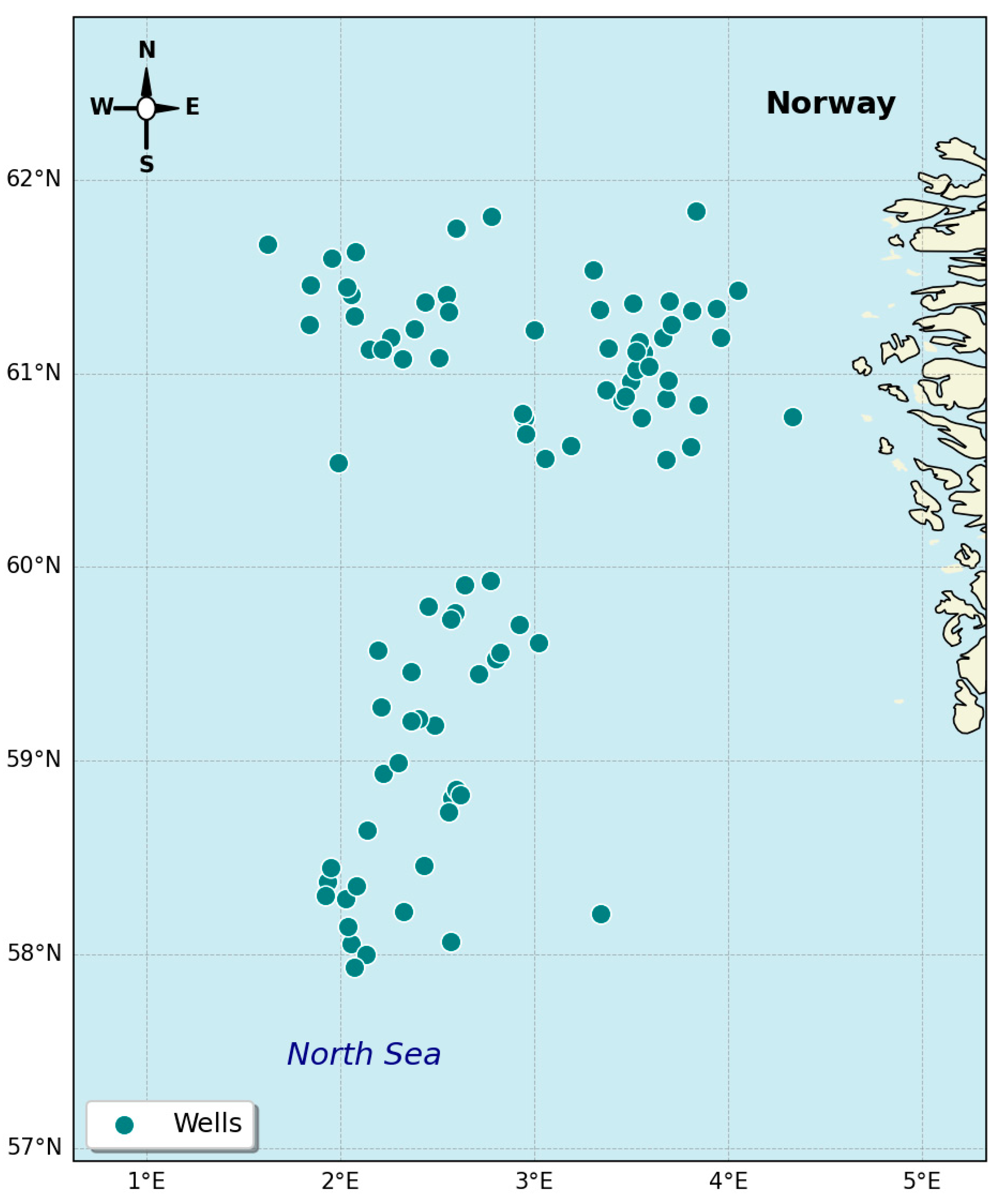
Figure 1. Geographic distribution of the wells.
Bdcc 10 00047 g001
Figure 2. Distribution of sample counts for the 12 lithology classes (facies) in the training set.
Bdcc 10 00047 g002
Figure 3. Heatmap of missing rates for different logging curves across wells (training and test sets).
Bdcc 10 00047 g003
Figure 4. Workflow of the Robust Feature Engineering (RFE) framework.
Bdcc 10 00047 g004
Figure 5. Illustration of the boundary sample set B used for Boundary F1 calculation. The shaded regions represent the specific neighborhoods where the metric is evaluated. The specific color codes corresponding to different lithologies are listed in Table 1.
Bdcc 10 00047 g005
Figure 6. Visualization of the FORCE 2020 [7,8,9] lithology penalty matrix. Darker colors indicate higher penalties for geologically implausible errors.
Bdcc 10 00047 g006
Figure 7. Performance comparison between Baseline XGBoost and the proposed RFE + XGBoost method. (a) Weighted F1 Score; (b) Boundary F1 Score; (c) Geological Penalty Score.
Bdcc 10 00047 g007
Figure 8. Comparison of row-normalized confusion matrices on the test set: (a) Baseline XGBoost and (b) the proposed RFE + XGBoost.
Bdcc 10 00047 g008
Figure 9. Comparison of model performance on feature-complete and feature-deficient wells under different missing-rate thresholds.
Bdcc 10 00047 g009
Figure 10. Model prediction case study on feature-complete wells from the independent test set: (a) Well 35/6-2 S; (b) Well 34/6-1 S. The specific color codes corresponding to different lithologies are listed in Table 1.
Bdcc 10 00047 g010
Figure 11. Robustness case study on incomplete data (severe missing intervals): (a) Well 29/3-1; (b) Well 25/5-3. The specific color codes corresponding to different lithologies are listed in Table 1.
Bdcc 10 00047 g011
Figure 12. Visual comparison of RFE feature engineering impact on prediction stability across different tree-based models (Random Forest, CatBoost, LightGBM) on Well 29/3-1. The specific color codes corresponding to different lithologies are listed in Table 1.
Bdcc 10 00047 g012
Table 1. Description of the 12 lithology classes.
Class of RockFaciesLabelColor
Sandstone0SS████
Sandstone/Shale1SS-Sh████
Shale2Sh████
Marl3Marl████
Dolomite4Dol████
Limestone5Lims████
Chalk6Chlk████
Halite7Hal████
Anhydrite8Anhy████
Tuff9Tuf████
Coal10Coal████
Basement11Bsmt████
Table 2. Ablation study on the effectiveness of Feature Engineering (FE) and Weighting strategies.
Model ConfigurationFEWeighingF1Penalty Score
Baseline (XGBoost)××66.35−0.7804
Baseline + Weighting×72.3−0.6346
Baseline + FE×72.59−0.6327
RFE + XGBoost72.72−0.6289
Table 3. Performance comparison under different data completeness conditions.
ProportionModelCom/IncomWeighted F1Boundary F1
0.1/0.4XGBoostComplete0.6990.385
0.1/0.4XGBoostIncomplete0.6400.371
0.1/0.4OursComplete0.7260.407
0.1/0.4OursIncomplete0.6830.387
0.2/0.5XGBoostComplete0.7050.390
0.2/0.5XGBoostIncomplete0.6340.357
0.2/0.5OursComplete0.7280.404
0.2/0.5OursIncomplete0.6860.378
0.3/0.6XGBoostComplete0.7060.394
0.3/0.6XGBoostIncomplete0.6080.341
0.3/0.6OursComplete0.7290.409
0.3/0.6OursIncomplete0.6620.367
Table 4. Performance Comparison of Different Tree Models With and Without Using RFE.
ModelF1Boundary F1Penalty Score
RF0.6918 0.3840−0.6776
RFE+RF0.7051 0.392−0.6467
CatBoost0.65010.3510 −0.7895
RFE+CatBoost0.68660.3725−0.7156
LightGBM0.6550 0.3768 −0.808
RFE+LightGBM0.70920.4147−0.6691
Disclaimer/Publisher’s Note: The statements, opinions and data contained in all publications are solely those of the individual author(s) and contributor(s) and not of MDPI and/or the editor(s). MDPI and/or the editor(s) disclaim responsibility for any injury to people or property resulting from any ideas, methods, instructions or products referred to in the content.