NovAc-DL: Novel Activity Recognition Based on Deep Learning in the Real-Time Environment

Abstract

Real-time fine-grained human activity recognition (HAR) remains a challenging problem due to rapid spatial–temporal variations, subtle motion differences, and dynamic environmental conditions. Addressing this difficulty, we propose NovAc-DL, a unified deep learning framework designed to accurately classify short human-like actions, specifically, “pour” and “stir” from sequential video data. The framework integrates adaptive time-distributed convolutional encoding with temporal reasoning modules to enable robust recognition under realistic robotic-interaction conditions. A balanced dataset of 2000 videos was curated and processed through a consistent spatiotemporal pipeline. Three architectures, LRCN, CNN-TD, and ConvLSTM, were systematically evaluated. CNN-TD achieved the best performance, reaching 98.68% accuracy with the lowest test loss (0.0236), outperforming the other models in convergence speed, generalization, and computational efficiency. Grad-CAM visualizations further confirm that NovAc-DL reliably attends to motion-salient regions relevant to pouring and stirring gestures. These results establish NovAc-DL as a high-precision real-time-capable solution for deployment in healthcare monitoring, industrial automation, and collaborative robotics.

1. Introduction

Deep learning has significantly advanced various domains, including image classification, speech recognition, natural language processing, and network traffic analysis [1,2]. While much of computer vision research has focused on static images, the importance of temporal dynamics in videos has been emphasized in early works on 3D convolutional and two-stream networks [3,4]. Many of these advancements have led to substantial improvements in tasks such as pattern recognition, sentiment analysis, and regression modeling [5]. Video data, characterized by their high volume and complexity, present unique challenges and opportunities for AI research. Platforms like YouTube have become invaluable resources, offering vast datasets for training and evaluation. However, the large file sizes and intricate temporal–spatial relationships inherent in video content necessitate specialized processing techniques [6]. While much of computer vision research has focused on static images, there is a growing recognition of the importance of video sequences. Videos provide richer context by capturing dynamic changes over time, offering deeper insights into actions and events. Digital video processing involves the automated analysis of video content, examining each frame to assess both temporal and spatial characteristics [7]. Figure 1 illustrates the nature of video data, highlighting the sequential and temporal aspects that differentiate them from static images. This distinction highlights the need for models that can understand and interpret the dynamic nature of video sequences.

In this work, NovAc-DL introduces a unified spatiotemporal deep-learning pipeline that integrates frame-level convolutional encoding with sequence-level temporal reasoning. Unlike standard HAR models developed for human-centered datasets, NovAc-DL is specifically tuned for robotic-hand motion and short fine-grained actions (“pour” and “stir”). Its novelty lies in the following: (i) a balanced robotic-condition video dataset, (ii) adaptive CNN-TD layers for low-latency spatial feature extraction, (iii) LSTM-based temporal fusion to preserve sequential consistency, and (iv) Grad-CAM interpretability that maps network attention to meaningful motion regions.

1.1. Related Works

Kansal et al. [8] utilized deep learning to classify human–robot interactions, while Zhu et al. [9] proposed a Modified Capsule Network (MCN) model for precise activity recognition. Another study [10] proposed CNN, ConvLSTM, and LRCN models [11] for human activity recognition (HAR) using video data from UCF50 and HMDB51, achieving accuracies up to 99.58% with CNN and demonstrating effective temporal feature extraction with ConvLSTM and LRCN for healthcare and surveillance applications. In manufacturing [12], integrating deep learning and computer vision for human action recognition and ergonomic risk assessment aims to improve workplace safety by accurately identifying and mitigating high-risk body movements through contextualized assistance systems. A three-stage deep learning architecture for anomaly detection in CCTV footage enhances accuracy and efficiency in complex and dynamic environments, promising advancements in security camera monitoring technologies [13]. Another work introduced a deep learning-based method to classify the Jellyfish sign in carotid artery plaques using ultrasound videos, validated on 200 patient cases [14].

Advanced techniques like M2RFO-CNN, BS2ResNet, LTK-Bi-LSTM, TSM-EfficientDet, and JS-KM with Pearson–Retinex are being used to address challenges in object detection, classification, and tracking in surveillance videos, particularly for dense and smaller objects in complex dynamic environments [15]. In cyberbullying detection, a thesis focused on multi-class classification using RoBERTa for text and ViT for images, achieving high accuracy and highlighting the effectiveness of a hybrid RoBERTa+ViT model [16]. Additionally, a hybrid model for detecting facemasks and hand gloves in images achieved high accuracy, ensuring pandemic safety in public places [17]. A new video classification model enhanced human behavior detection with a multi-scale dilated attention mechanism and gradient flow feature fusion, demonstrating significant accuracy improvements over existing models [18]. The CNN processes data from nine activities, classifying them based on unique movement patterns and changes in joint distances across consecutive frames within each activity segment, using the Euclidean distance [19]. A robust HAR system was developed by merging deep learning and signal processing to leverage data from wearable sensors effectively [20]. A new method for recognizing human activities combined a multi-head CNN with CBAM for visual data analysis and a ConvLSTM for time-sensitive sensor data, utilizing multi-level feature fusion to integrate information from various sources [21].

Furthermore, a hybrid approach to semi-supervised classification employing Encoder-Decoder CNNs integrated privately obtained unlabeled raw sensor data with publicly available labelled raw sensor data [22]. Systematic literature reviews on deep learning in video processing have examined applications, functionalities, techniques, datasets, concerns, and obstacles, highlighting the need for further research [23]. Studies on transfer learning using CNNs and RNNs for video classification have shown improvements in accuracy with ConvLSTM-based classifiers [24]. The use of 3D CNNs, addressing both spatial and temporal features, enhances accuracy in video analysis compared to 2D CNNs [25]. In sports training, deep learning models achieve high accuracy and improved speed via event matching [26].

Privacy-aware video classification methods based on Secure Multi-Party Computation have been applied to emotion recognition, achieving high accuracy across diverse security scenarios [27]. Reviews of recent advancements in deep learning models for video classification emphasize key findings, network architectures, evaluation criteria, and datasets, proposing future research directions [28]. Novel CNN architectures enhanced echocardiography interpretation, reducing the error rate and approaching expert accuracy [29]. Deep convolutional networks have achieved success in image recognition. However, for action recognition in videos, their advantage over traditional methods is not as evident [30].

Incorporating an attention mechanism and long short-term memory networks, deep learning precisely classified freestyle gymnastics movements in videos, enhancing the user experience in sports video classification [31]. New mobile video processing and LSTM-SRNN deep learning models accurately predicted rice plant diseases, demonstrating dynamic learning adaptability [32,33]. A technique for understanding decisions made by 3D CNNs in video classification utilized a 3D occlusion mask that dynamically adjusts based on temporal–spatial data and optical fluxes, outperforming standard methods [34].

Deep learning techniques for analyzing lung ultrasounds in resource-constrained contexts accurately identified pleural effusion, lung consolidation, and B-lines, providing expert-level support for detecting pneumonia [35]. One study proposed a framework based on deep learning to classify sports videos with their appropriate class label. The framework is to perform sports video classification using two different benchmark datasets, UCF101 and the Sports1-M dataset [36]. An unsupervised method combining CNN and temporal segment density peak clustering improved key frame extraction and video classification, outperforming state-of-the-art findings [37]. Digital Twin (DT) technology, combining data analytics and multi-physics modeling, enhanced risk assessment and worker safety by identifying high-risk scenarios [38,39].

Gesture recognition literature has applied a ResNet-50 model to hand hygiene steps, achieving notable accuracy. Future efforts will focus on expanding the dataset and classes [40]. Deep learning has been used to classify human skeleton behavior in movies, improving data labeling and achieving high accuracy [41]. CNNs and RNNs accurately predicted droplet sizes in agricultural spray solutions [42]. A robust algorithm for identifying orchard fruits using video processing and hybrid neural networks achieved high accuracy through majority voting with diverse classifiers [43]. The suggested method for medical video analysis combined detection and classification, providing good interpretability with minimal frame-level monitoring and increasing localization for predicting lung consolidation and pleural effusion [44]. Finally, MOV, a novel approach to multimodal open-vocabulary video categorization, incorporated video, optical flow, and audio into pre-trained vision–language models with minimal changes, setting new standards for zero-shot video categorization [45].

1.2. Motivation

This research aims to create a model that can reliably recognize “pour” and “stir” motions from sequential still images taken from recordings, creating the foundation for a complex comprehension of ongoing human activities. This research has important applications in the real world:

• The model could improve surveillance systems by distinguishing between typical activity and questionable behavior, such as unauthorized pouring or stirring in forbidden regions.
• Recognizing certain behaviors in aged care could alert carers to atypical behaviors, enhancing patient monitoring and responsiveness.
• Identifying specific vehicle activities to prevent accidents and promote safer driving practices.
• Optimizing production by automating quality control by recognizing pour and stir activities.

1.3. Contribution

The study presents the design and assessment of multiple Human Activity Recognition (HAR) models for classifying fine-grained daily actions such as pour and stir. It explores three spatial–temporal learning architectures, namely, Long-term Recurrent Convolutional Network (LRCN), Time-Distributed Convolutional Neural Network (CNN-TD), and ConvLSTM, to investigate how temporal dependencies and spatial features can be effectively modeled.

• We introduce NovAc-DL, a unified deep learning framework for fine-grained robotic action recognition using real-world “pour” and “stir” tasks, bridging human–robot collaboration domains.
• We conduct a comparative evaluation of three distinct spatiotemporal models, i.e., LRCN, ConvLSTM, and CNN-TD under identical dataset and preprocessing settings, providing quantitative insight into spatial vs. temporal representation strengths.
• We provide interpretability through Grad-CAM visualization, linking motion-specific activations to the physical regions of action (e.g., container–target interface during pouring and cyclic motion in stirring).

The remainder of this paper is organized as follows. Section 2 describes the used dataset. Section 3 describes the suggested methods. Section 4 expands on the results and discussions. Section 5 summarizes the findings and provides concluding remarks.

2. Related Dataset

2.1. Data Set Description

The data used for this research consist of a comprehensive collection of videos carefully curated to understand and evaluate human activity recognition. Specifically, the dataset features two primary activities: ‘pour’ and ‘stir’. All videos were captured at 30 fps and 640 × 480 resolution from three fixed viewpoints (front, left-oblique, overhead) under mixed indoor lighting conditions. Action boundaries were manually annotated by three experts based on visible motion onset and tool–target completion, with an inter-annotator agreement = 0.94 (Cohen’s (k)).

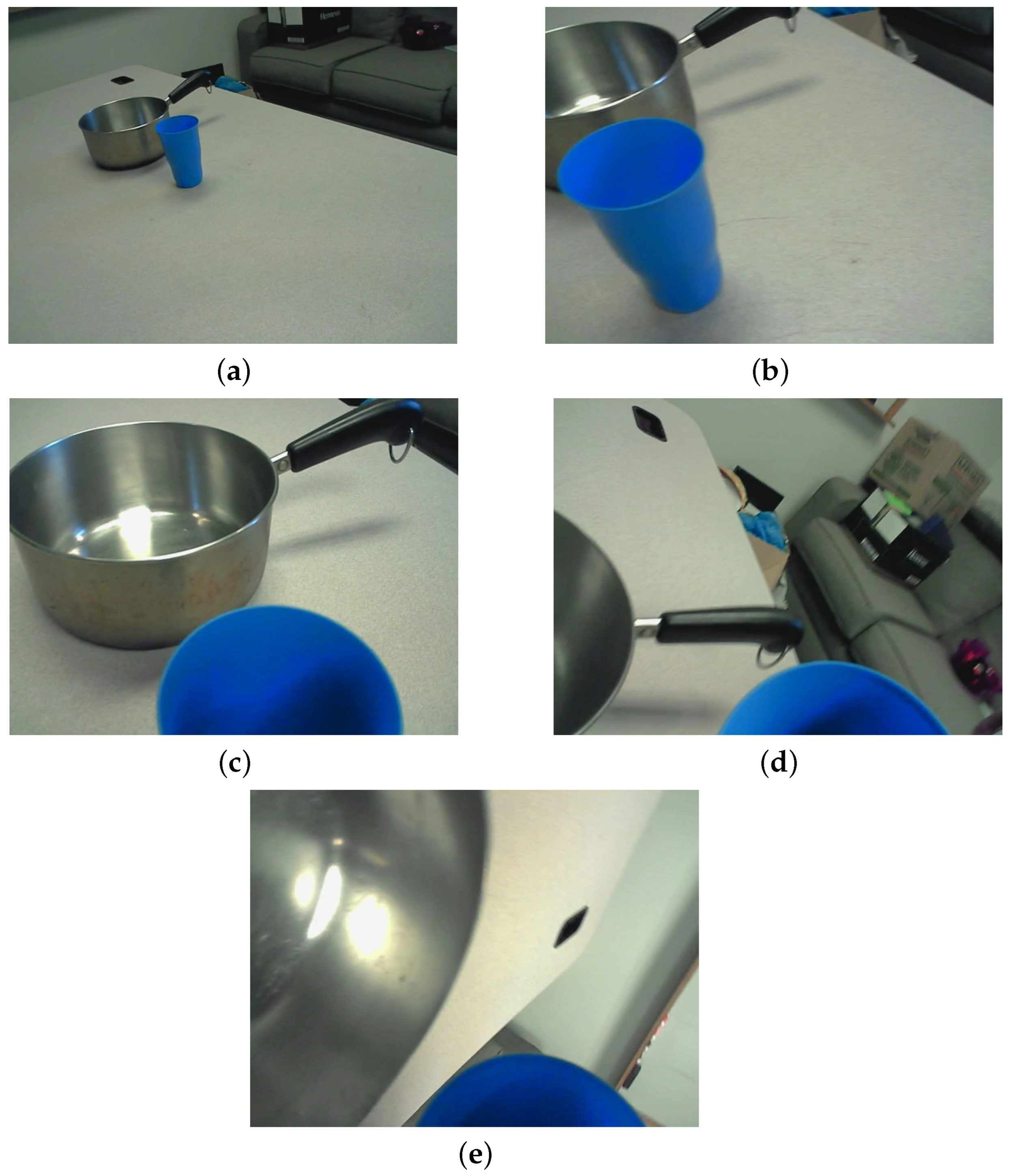
A total of 1000 videos represent the ‘pour’ activity [46]. Reference benchmark datasets such as UCF50 and HMDB51 [47,48] were also considered during dataset validation. These videos encompass a range of scenarios and conditions to capture the variety and complexity inherent in the act of pouring. They include different subjects, pouring techniques, container types, and pour materials. All these factors contribute to creating a well-rounded and robust dataset that challenges and refines the recognition models developed. An example sequence of frames from the ‘pour’ class is shown in Figure 2.

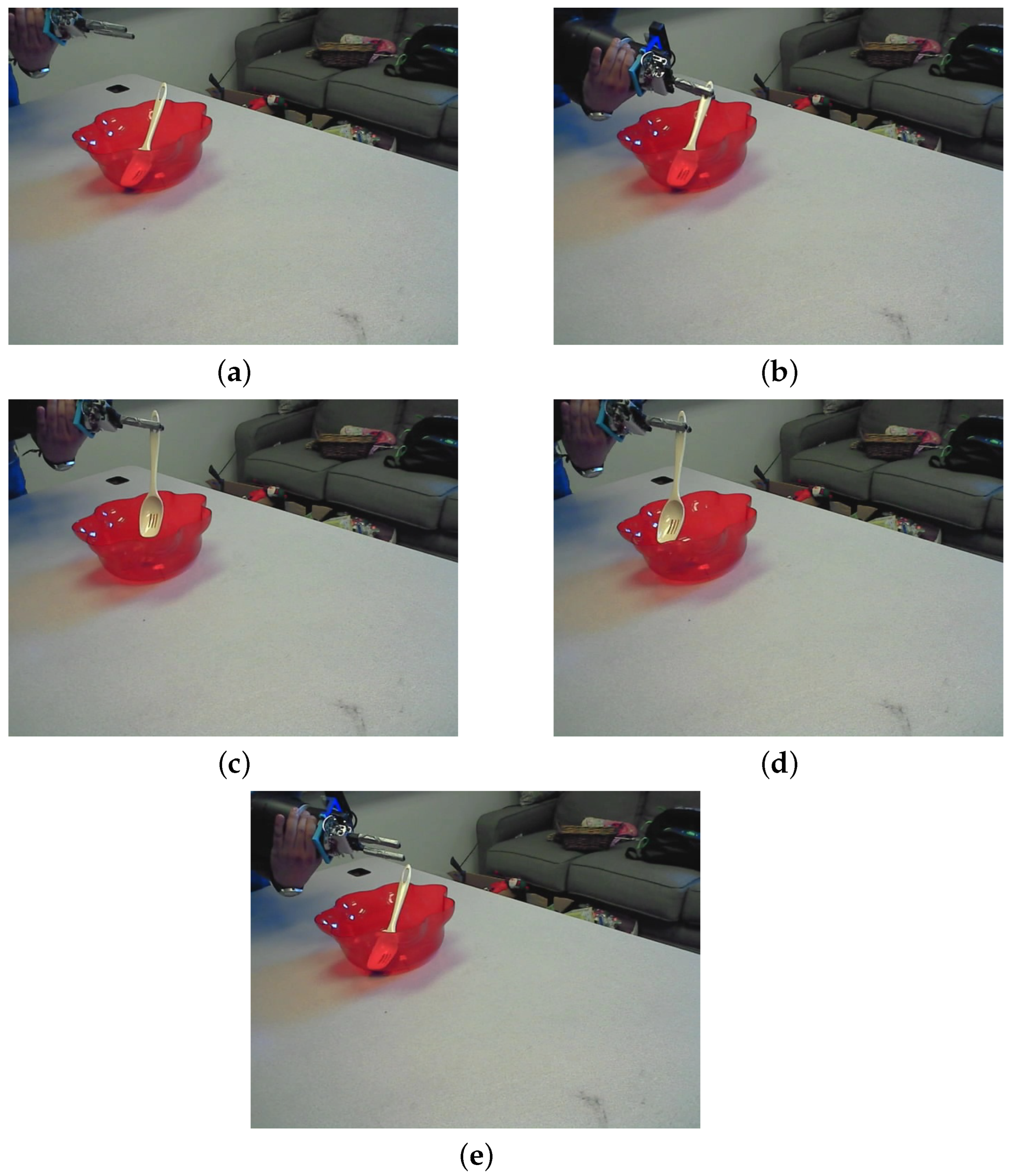
On the other hand, the ‘stir’ activity is represented by twice the amount, with a total of 2000 videos. This larger sample size was necessary to adequately capture the higher complexity and variation in the stirring activity. As with the ‘pour’ videos, these also feature various scenarios, subjects, stirring techniques, utensils, and materials being stirred. From each video, we extracted frames in a time-series order to maintain the temporal aspect of the tasks. These frames, effectively convert the videos into image sequences, allowing us to leverage video-based and image-based activity recognition advantages. An example sequence of frames from the ‘stir’ class is shown in Figure 3. By preserving proper timestamps, we ensured the temporal coherence and the sequence of the actions, enabling the research to account for the temporal dynamics of the ‘pour’ and ‘stir’ activities.

2.2. Data Preprocessing

Frames were extracted at uniform intervals using OpenCV routines, resized to 224 × 224 pixels, and normalized to [0, 1], following preprocessing standards used in recent HAR literature [10,37]. Background cropping was omitted to preserve the spatial context. The function includes exception handling to skip unreadable frames and dynamically resample sequences to a uniform length of 30 frames per video. In the preprocessing phase of our research, we faced the challenge of data imbalance, which commonly occurs when certain classes are over-represented compared to others. In our dataset, the ‘pour’ activity consisted of 1000 videos, while the ‘stir’ activity had 2000 videos. Training models on such imbalanced data can bias them towards the majority class, leading to poor generalization and inflated performance metrics for the under-represented class.

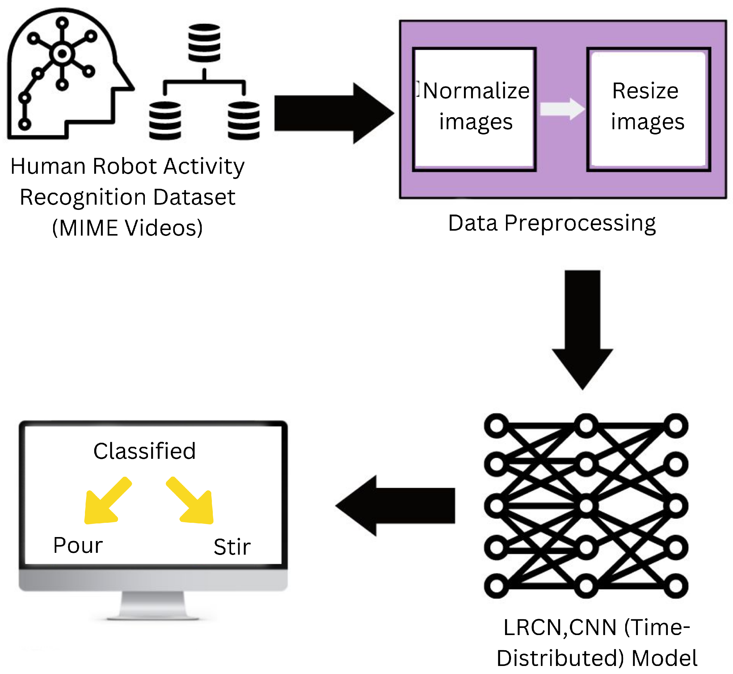
To mitigate this issue and ensure that our models were trained on a balanced dataset, we reduced the number of ‘stir’ videos to match that of the ‘pour’ videos, resulting in 1000 videos for each class. The 1000 videos from the original ‘stir’ set were selected using a random sampling strategy, where each video had an equal probability of being chosen. Pilot tests with class-weighted loss functions produced unstable convergence (±1% accuracy variance). This approach ensured that the selected subset accurately represented the overall diversity of the full class, including variations in subjects, stir techniques, utensils, materials, and camera angles. Random selection was preferred over sequential or manual selection to minimize the introduction of unintended biases related to specific scenes, subjects, or recording conditions. By preserving the temporal and spatial diversity of the original ‘stir’ dataset, this strategy supports robust learning for sequence-based models such as LRCNs and CNN-TD, as illustrated in Figure 4. Now, the preprocessing steps encoded in our create_dataset function are as follows:

• Initialize three empty lists: features, labels, and video_files_paths.
• For each class in CLASSES_LIST (which, in our case, would be ‘pour’ and ‘stir’), print out the class currently being processed.
• For each file in the directory of the current class, create the full path to the file and extract the frames from the video using the frame_extractor function.
• Append the extracted frames to the features list, the class index to the labels list, and the video file path to the video_files_paths list. The class index is derived from the enumeration of CLASSES_LIST.
• After all videos have been processed, the features and labels lists are converted into NumPy arrays, a more efficient data structure for subsequent data processing and modeling tasks.
• Finally, the function returns the features, labels, and video_files_paths. At the end of this function, features will contain all the frames of all the videos in a structured format, labels will contain the corresponding class labels, and video_files_paths will contain the file paths of the videos.

The function create_dataset effectively transforms the raw video files into a structured format ready for model training and testing, while addressing the initial data imbalance issue by equalizing the number of videos used for each activity. Algorithm 1 outlines the process of extracting frames from a video and determining skip intervals for even sampling. Frames are resized, and pixel values are normalized, forming a dataset for machine learning or computer vision tasks. It offers a systematic video preprocessing approach.

Algorithm 1 Uniform Frame Extraction and Preprocessing

Require: video_path, desired_length $L=30$, target size $(224,224)$ Ensure: A sequence of at most L preprocessed frames   1: Initialize an empty list F   2: Load the input video from video_path   3: $T\leftarrow$ total number of frames in the video   4: $s\leftarrow max\left(⌊{\displaystyle \frac{T}{L}}⌋,1\right)$                      ▹ Sampling interval   5: for $i=0$ to $L-1$ do   6:      Set video position to frame index $i\times s$   7:      Read a frame from the video   8:      if frame read fails then   9:           break   10:    end if   11:    Resize the frame to $(224,224)$   12:    Convert pixel values to the range $[0,1]$ (normalization)   13:    Append the normalized frame to F   14: end for   15: return  F

3. Proposed Methods and Descriptions

3.1. Long-Term Recurrent Convolutional Networks (LRCN)

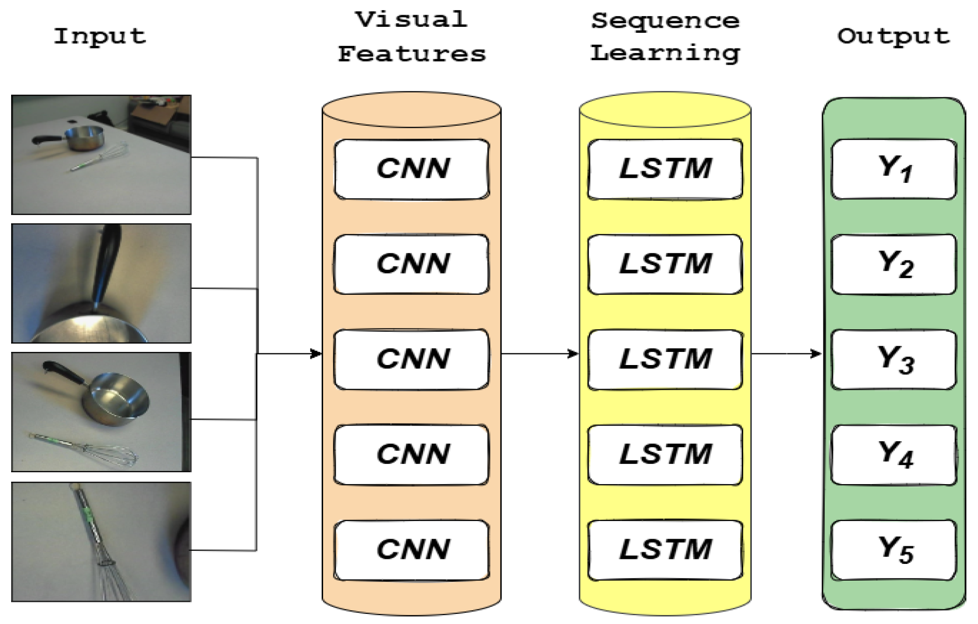
The LRCN architecture employed combines CNN feature extraction with LSTM-based temporal modeling, originally introduced in [11]. Convolutional and recurrent neural networks are used in the LRCN model, with CNNs extracting characteristics from individual video frames and RNNs capturing temporal relationships between frames. The LRCN model was constructed using Keras, a high-level neural network API, and TensorFlow as a backend. The VGG16 model [49] functioned as a feature extractor for individual frames after being pre-trained on the ImageNet dataset. The fully connected layers of VGG16 were removed, and the remaining convolutional layers were used as a feature extractor for each frame in the video. The VGG16 model was applied to every frame in the video sequence using the time-distributed layer. The model design also includes a flattened layer and two convolutional layers, each followed by an activation function known as a Rectified Linear Unit (ReLU) [50]. The output of the time-distributed layer was fed into these layers, which extracted more abstract features from the individual frames. The flattening output was fed into an LSTM layer, which preserves frame temporal correlations (Figure 5). Several classes were created from the action in the video by applying a dense layer with a softmax activation function. We trained multiple LRCN models with different initialization and hyperparameters to improve the generalization performance. With the help of the Adam optimizer [51] and the definite cross-entropy loss function, we trained five models, each with a separate random initialization. To stop the model from being over-fitted, we also used early stopping. We monitored the accuracy of the validation set. If it did not improve for ten epochs, we stopped training the model and used the weights with the highest validation accuracy. To combine the predictions of the multiple LRCN models, we used the majority voting ensemble technique. For each test video, we made predictions using each of the five trained models and then selected the most common prediction as the final prediction. The mathematical formulations are as follows.

The sigmoid and tanh functions used in the LSTM cells are shown in Equations (1) and (2).

$$\sigma \left(x\right)={\displaystyle \frac{1}{1+e^{-x}}}$$

(1)

$$tanh\left(x\right)={\displaystyle \frac{e^x-e^{-x}}{e^x+e^{-x}}}$$

(2)

• Input Gate: The input gate’s job is to add filtered data from the current input to the knowledge already learned. Equations (3) and (4) show the input gate and candidate layer output, where $x_t,h_{t-1}$ are the current input and previous hidden state, while W and U are the weights.

  $$i_t=\sigma (x_t{U}^i+h_{t-1}{W}^i)$$

  (3)

  $$S_t=tanh(x_t{U}^g+h_{t-1}{W}^g)$$

  (4)
• Output Gate: Calculating the output $o_t$ and hidden output $h_t$ is the goal of this gate. These are computed using Equations (5) and (6).

  $$o_t=\sigma (x_t{U}^o+h_{t-1}{W}^o)$$

  (5)

  $$h_t=tanh\left(C_t\right)\ast o_t$$

  (6)
• Forget Gate: This gate decides which data from the earlier states will be removed from the cell memory. This is computed using Equation (7).

  $$f_t=\sigma (x_t{U}^f+h_{t-1}{W}^f)$$

  (7)
• Cell Memory: The vital information from previous states is stored within the cell memory to prevent data loss due to diminishing gradients. Each LSTM cell continually updates the cell memory using Equation (8), wherein $C_t,C_{t-1},f_t,i_t,S_t$ denote the current memory state, previous memory state, output of the forget gate, output of the input gate, and output of the candidate layer, respectively.

  $$C_t=\sigma (f_t\ast C_{t-1}+i_t\ast S_t)$$

  (8)

3.2. CNN-TD

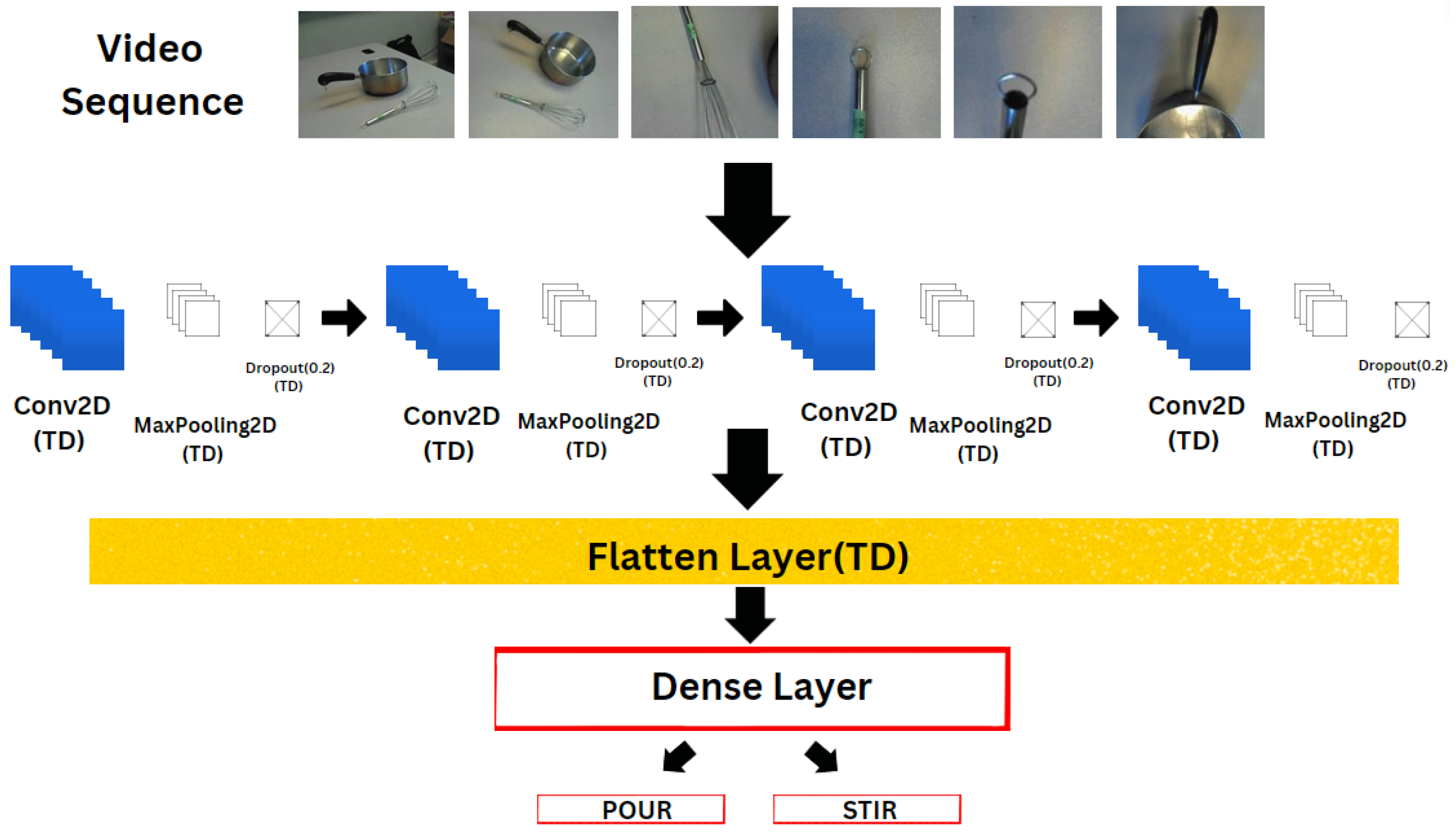
The model architecture utilized in this study draws from several key layers available in the ‘keras.layers’ module, including ‘Conv2D’, ‘MaxPooling2D’, ‘Dense’, ‘Flatten’, ‘Dropout’, and ‘TimeDistributed’. Each layer contributes uniquely to the process of feature extraction, dimensionality reduction, and classification, forming an integrated deep learning pipeline for spatiotemporal data analysis. In particular, the convolutional layers (‘Conv2D’) are responsible for identifying visual patterns, while the pooling and dropout layers ensure efficient learning and generalization. The dropout is placed after the final Conv2D block and before the dense layer, which precedes classification. The combination of these layers, wrapped within the ‘TimeDistributed’ structure, enables the model to process sequences of image frames in a video and capture both spatial and temporal dependencies effectively.

The Conv2D layer is central to the network’s feature extraction process. It operates through filters, also referred to as kernels, which are small matrices that slide over the input data to detect meaningful patterns such as edges, textures, or complex shapes. Each filter learns to specialize in recognizing a specific feature, making the layer capable of building a hierarchical understanding of the input images. The kernel size determines the receptive field of each neuron; larger kernels capture broader, more global features, while smaller ones focus on fine, local details. Proper configuration of the padding and stride parameters ensures the spatial dimensions are maintained or reduced appropriately. When “padding = same” with a stride of 1, the spatial resolution of the output remains consistent with the input, preserving critical information at the image boundaries. An important component of Conv2D layers is the activation function, which introduces non-linearity into the model. The Rectified Linear Unit (ReLU) is employed here because of its simplicity and efficiency, defined mathematically as $\left(f\right(x)=max(0,x\left)\right)$. This function effectively zeroes out negative values while retaining positive activations, leading to sparse representations and faster convergence during training. ReLU enhances the network’s ability to model complex non-linear relationships while preventing issues such as the vanishing gradient problem commonly encountered with older activation functions like sigmoid and tanh.

Following convolutional operations, the MaxPooling2D layer performs spatial downsampling to reduce the computational load and the number of parameters. This layer divides the feature map into non-overlapping sections, defined by the pool size (commonly $(2\times 2)\mathrm{or}(3\times 3))$ and selects the maximum value from each region. By retaining the most prominent features and discarding less informative details, MaxPooling2D helps the model focus on the most significant spatial cues, improving both the robustness and translation invariance. This reduction in spatial resolution also mitigates overfitting and accelerates training. To further regularize the network, a Dropout layer is incorporated. During training, dropout randomly sets a fraction (e.g., 20%) of input neurons to zero at each iteration, effectively omitting them from both forward and backward passes. This stochastic exclusion forces the model to develop redundant pathways for learning, resulting in better generalization when tested on unseen data. Importantly, dropout is only applied during training—during inference, all neurons are active, but their outputs are scaled according to the dropout probability used earlier.

Finally, the inclusion of the TimeDistributed wrapper is crucial for handling video data. Since conventional CNNs are designed for 2D image processing, "TimeDistributed" applies the same convolutional operations independently to each frame within a sequence, preserving spatial features at the frame level. These features are then passed to recurrent or sequential layers (e.g., LSTM, ConvLSTM) to capture temporal correlations between frames. In summary, this architecture, as shown in Figure 6, allows the convolutional model to process both spatial and temporal characteristics, making it particularly well-suited for video-based HAR tasks that require distinguishing fine-grained motion patterns over time.

3.3. ConvLSTM (CNN-3D)

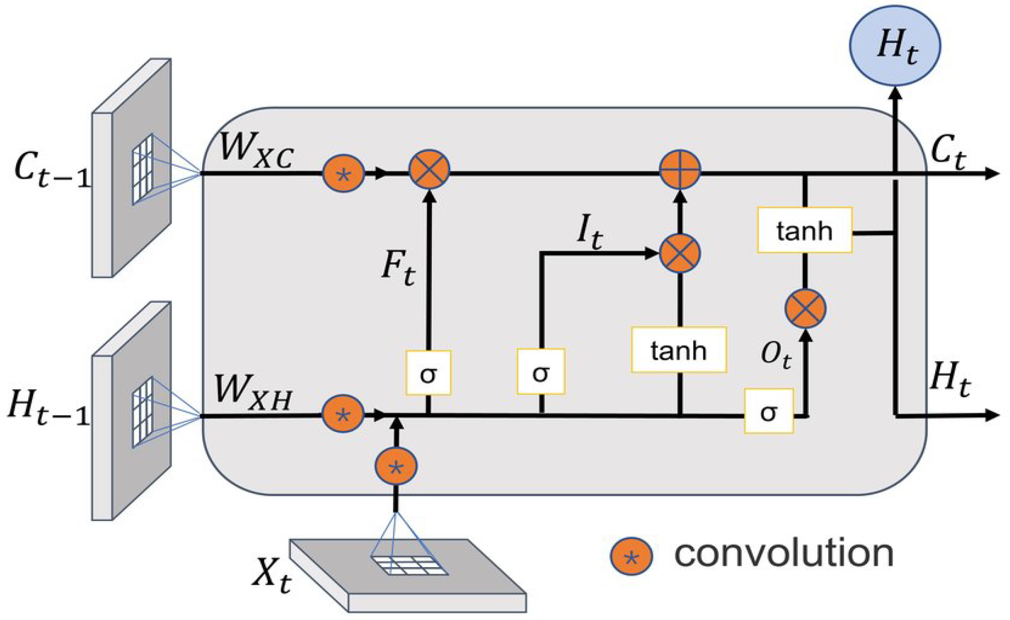
The ConvLSTM layer formulation follows the approach proposed in [52], preserving spatial dependencies through convolutional gating. The main weakness of the fully connected-LSTM is the use of full connections during the input state and state-to-state transitions, which leads to extensive information loss. To solve this problem, our design uses the ConvLSTM approach. In ConvLSTM, $x_1,\dots ,x_t$ produces the output C₁, …, C_t. Hidden state H₁, …, H_t, and gate IT, FT, OT are spatial dimension 3D tensors representing vectors in the set. Because of this structure, ConvLSTM can forecast a given cell’s future state by considering the previous states of nearby cells in the input and configuration. Spatial relationships are preserved by using convolution operators when transitioning from state to input, simplifying the process (see Figure 7). The ConvLSTM Equation (9) is shown below, where “*” is the convolution operator, and “o” stands for the Hadamard product.

$$\begin{array}{cc}\hfill i_t& =\sigma (W_{xi}{x}_t+W_{hi}{H}_{t-1}+W_{ci}\odot C_{t-1}+b_i)\hfill \\ \hfill f_t& =\sigma (W_{xf}\ast x_t+W_{hf}\ast H_{t-1}+W_{cf}\odot C_{t-1}+b_f)\hfill \\ \hfill C_t& =f_t\odot C_{t-1}+i_t\odot tanh(W_{xc}\ast x_t+W_{hc}\ast H_{t-1}+b_c)\hfill \\ \hfill o_t& =\sigma (W_{xo}\ast x_t+W_{ho}\ast H_{t-1}+W_{co}\odot C_t+b_o)\hfill \\ \hfill H_t& =o_t\odot tanh\left(C_t\right)\hfill \end{array}$$

(9)

It can take faster action in the hidden representation of moving objects. Smaller cores, on the other hand, can record slower movements. The problem is that the inherently spatiotemporal map box is divided into non-overlapping patches, and each patch’s size is displayed per pixel (see Figure 7). Padding is required before the draw procedure to ensure that the states’ ranks are equal and columns are inputs. In LSTM-based sequence modeling, initialization at $(t=0)$ represents a state of temporal uncertainty, where no prior context exists. To handle this, zero padding is applied to the initial hidden and cell states, serving as a neutral boundary condition that isolates the model from any external or unobserved influences. This ensures that the network’s temporal dependencies are learned purely from the observed input sequence. Conceptually, zero padding acts like a boundary around a dynamic system, similar to a ball moving within walls, preventing undefined state propagation beyond the observable domain while maintaining stable and consistent state transitions within it.

3.4. Model Architecture and Hyperparameters

The LRCN architecture utilised a VGG16 network pre-trained on ImageNet as the spatial feature extractor, with the classification head removed and only the convolutional layers retained. To balance efficiency and adaptability, the first ten convolutional layers were frozen while the final five were fine-tuned, enabling the model to refine higher-level spatial representations relevant to the “pour” and “stir” activities. Frame-level features generated by VGG16 were then passed to an LSTM module with 256 units, enabling the system to capture the temporal dynamics essential for activity recognition.

Five independent LRCN models were trained using random seeds (0, 7, 21, 37, 45), all sharing the same hyperparameter configuration: a 64-unit LSTM layer, 0.5 dropout, a 64-unit dense layer followed by a 3-class softmax, a learning rate of $(1\times {10}^{-4})$, and a batch size of 32. Majority-voting fusion across these models improved the mean test accuracy from (98.50% ± 0.12) to (98.68%), demonstrating a modest but consistent enhancement in generalization performance.

For the CNN-TD model, the complete architecture consists of three Conv2D layers with 64, 128, and 256 filters, respectively, each with a $3\times 3$ kernel, followed by a $2\times 2$ maxpooling layer and a dropout rate of 0.2. These components were chosen to progressively capture spatial hierarchies while controlling overfitting. The ConvLSTM model consisted of a single ConvLSTM layer with 64 filters, $3\times 3$ kernels, ReLU activation, and a dropout rate of 0.1, balancing spatiotemporal representation with computational cost.

Frames were initially resized to 224 × 224 as part of the standard preprocessing description inherited from the VGG16-based feature extractor used in LRCN. However, in the finalized and unified NovAc-DL pipeline, all videos were uniformly downsampled to 15 frames, and each frame was resized to 64 × 64 × 3, serving as the actual input size for all three models: LRCN, CNN-TD, and ConvLSTM. This ensured architectural comparability and consistent computational cost. The training hyperparameters for all models were batch size of 16, learning rate of $1\times {10}^{-4}$, Adam optimizer ( ${\beta }_1=0.9,{\beta }_2=0.999$, $ϵ=1\times {10}^{-7}$), and 40 training epochs. The dataset was partitioned into 64% for training, 16% for validation, and 20% for testing. This allocation was obtained by first performing an 80:20 train–test split, after which 20% of the training portion was further separated to form the validation set.

4. Results

4.1. Training Performance

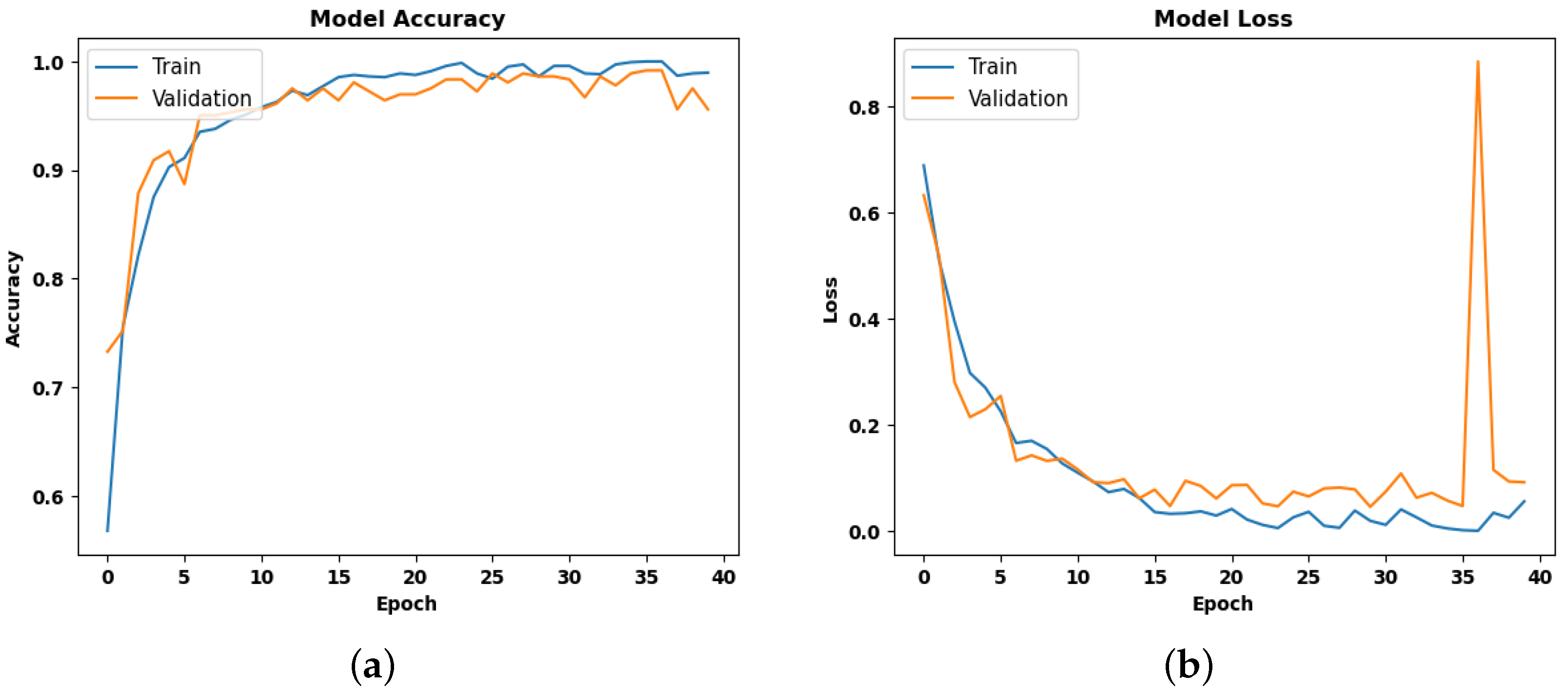
As shown in

Table 1. Comparison of validation loss and validation accuracy values obtained from LRCN, CNN-TD, and ConvLSTM models across different epochs.

Sr. No.	Model	Epoch	Validation Loss	Validation Accuracy
1	LRCN	10	0.1314	0.9559
		20	0.0920	0.9725
		40 (Last)	0.0403	0.9917
2	CNN-TD	10	0.0806	0.9697
		20	0.0395	0.9890
		32 (Early Stop)	0.0533	0.9890
3	ConvLSTM (3D-CNN)	10	0.1217	0.9669
		20	0.1766	0.9725
		40 (Last)	0.2345	0.9587

, after running this model on the training dataset, we obtained the best validation accuracy from the Time-Distributed Convolutional Neural Networks (CNN-TD), followed by the Long-term Recurrent Convolutional Networks (LRCN) and ConvLSTM models. Following a similar trend, we can conclude that CNN-TD has the smallest validation loss among all the models we have used, followed by LRCN, and finally, with a considerable jump, ConvLSTM (CNN-3D), especially at epochs 20 and 40. The CNN-TD reached convergence in 32 epochs, whereas the LRCN and ConvLSTM models required the full training cycle. The CNN-TD consistently improved accuracy with each epoch, effectively capturing the intricate temporal dynamics present in the video data. As we analyze the graphs we have plotted for all the models, we can see that the ConvLSTM has the worst accuracy compared to the validation accuracy and loss, with overlapping curves. Overall, the CNN-TD model demonstrated superior performance. It effectively captured spatial and temporal information, providing a more comprehensive understanding of human actions in videos.

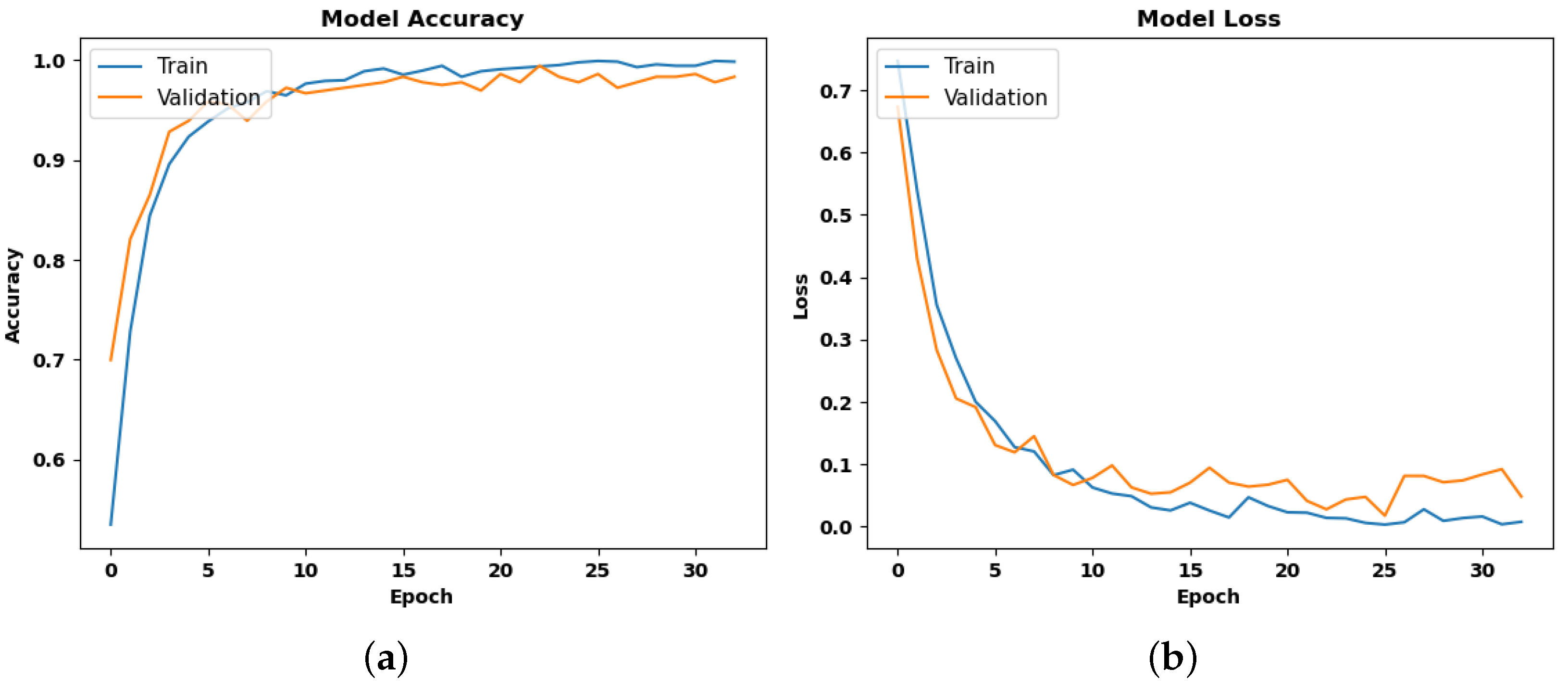
Figure 8 illustrates the training dynamics of the CNN-TD. Subfigure (a) shows a steady increase in both the training and validation accuracy, converging near 0.99, while subfigure (b) presents a rapid decline and stabilization of loss values within 32 epochs due to early stopping. The best weights correspond to the epoch with the highest validation accuracy, confirming that model saving was based on maximum validation accuracy and not minimum validation loss. This means that training continued until no further improvement was observed in the validation accuracy, after which the model stored the checkpoint with the peak performance. The smooth and parallel trajectory of the accuracy and loss curves indicates excellent generalization and minimal overfitting. The CNN-TD architecture effectively models spatial–temporal dependencies across frames, resulting in superior convergence speed and predictive reliability compared to other models.

Figure 9 shows that the LRCN model exhibits gradual convergence, achieving an accuracy of 0.98–0.99 after 40 epochs. The slight gap between training and validation curves suggests minor overfitting attributed to recurrent complexity and longer sequence dependencies. While the LSTM layers enable robust temporal feature learning, the model demands higher training time and parameter tuning. Nevertheless, it maintains high classification accuracy and stable learning, confirming the suitability of recurrent–convolutional hybrids for sequence modeling.

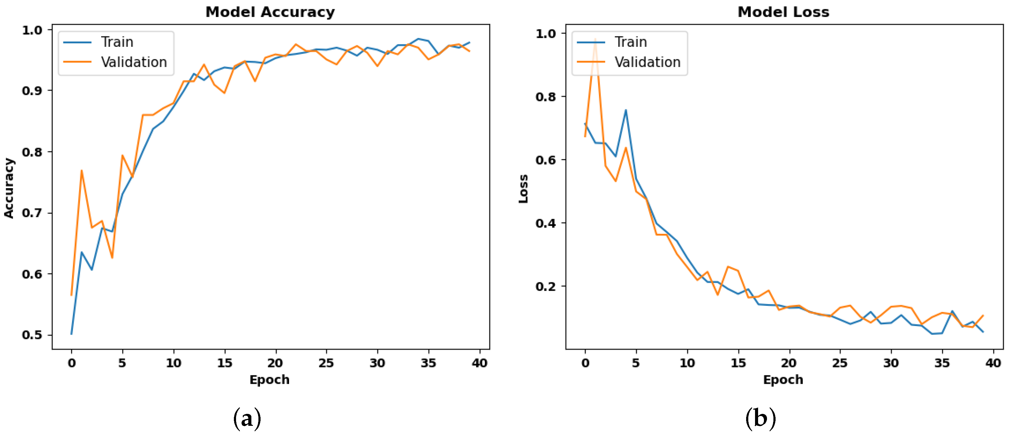
Figure 10 presents the performance of the ConvLSTM model. Both training and validation metrics exhibit oscillations, reflecting learning instability and slower convergence due to the heavy 3D convolutional operations. The final validation accuracy of approximately 97% and comparatively higher loss values suggest limited temporal generalization under the available computational resources. This observation underscores the trade-off between representational richness and computational overhead in 3D spatiotemporal networks.

4.2. Testing Performance

As shown in

Table 2. Comparison of model performance metrics.

No.	Model	Loss	Accuracy	Precision	Recall	F1
1	LRCN	0.0574	0.9868	0.978	0.975	0.975
2	CNN-TD	0.0236	0.9868	0.982	0.982	0.981
3	ConvLSTM	0.1236	0.9736	0.967	0.965	0.965

, evaluation on the testing dataset reveals that both the LRCN and CNN-TD models achieve the highest accuracy, with minimal differences between them. The CNN-TD model achieved the highest precision (98.2%), recall (0.982%), and F1-score (0.981%), outperforming LRCN and ConvLSTM. In contrast, the ConvLSTM (CNN-3D) model lags behind, exhibiting a noticeable drop in performance. All performance metrics are computed using macro-averaging of scikit-learn [53]. These results confirm that the LRCN and CNN-TD models generalize effectively to unseen data, maintaining robust activity recognition capabilities, while the ConvLSTM (CNN-3D) model is comparatively less effective in capturing the temporal and spatial dynamics.

The CNN-TD demonstrated the most effective handling of spatial–temporal dynamics, achieving 98.68% accuracy with the lowest validation loss. Its frame-wise convolutional processing enables parallel extraction of spatial features while minimizing redundancy between consecutive frames, directly supporting its claimed computational efficiency for real-time deployment. In contrast, the LRCN, which relies on sequential recurrent gating to capture temporal evolution, showed stable but slower convergence, consistent with the higher temporal processing overhead inherent to recurrent architectures. ConvLSTM’s reduced accuracy (97.36%) results from its high parameter count (10.2 M) and the heavy cost of 3D convolutions, leading to partial under-training within 40 epochs. Increasing the training length to 60 epochs produced <0.2% improvement, confirming the architecture’s inefficiency for short temporal motions. These observations collectively confirm that architectures optimized for efficient spatiotemporal feature separation and reduced computational load demonstrate superior convergence behavior and generaliaation performance in this task.

Although the CNN-TD and LRCN models both achieved identical test accuracy (98.68%), their loss values differ significantly (CNN-TD) = 0.0236 vs. LRCN = 0.0574). This discrepancy occurs because accuracy only measures whether the final class prediction is correct, whereas cross-entropy loss captures the confidence of those predictions. In the LRCN architecture, the LSTM layer smooths temporal probabilities, generating more conservative softmax outputs. These less-confident predictions still yield correct labels, maintaining accuracy but increasing loss due to reduced confidence. In contrast, CNN-TD performs direct frame-level convolutional encoding without recurrent smoothing, producing sharper and higher-confidence class probabilities, thereby reducing loss. Thus, the difference in test loss does not contradict identical accuracy; rather, it highlights the variation in confidence calibration and temporal smoothing between the architectures, implying that CNN-TD offers better confidence generalization for this task.

4.3. Experimental Analysis

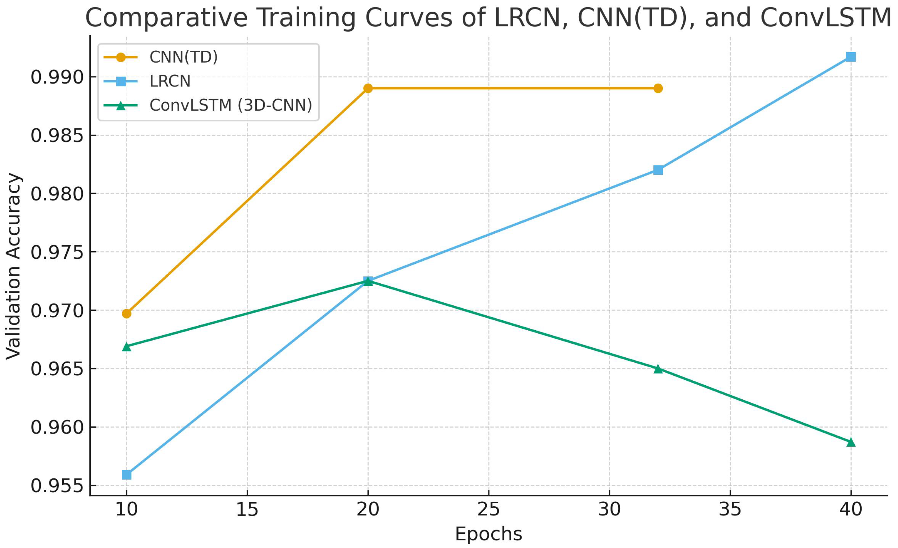
By varying the number of Conv2D filters (64 to 512) in CNN-TD, it was observed that the accuracy improved up to 256 filters but saturated beyond this point due to increased computational overhead. The parameter deviation $(\mathrm{\Delta }\theta <3\%)$ confirmed stable convergence for CNN-TD, while LRCN (≈$5\%$) and ConvLSTM (≈$9\%$) exhibited higher variance owing to recurrent and 3D convolutional complexity. A comparative training-curve analysis, as shown in Figure 11, directly contrasts the convergence patterns of all three models and highlights clear differences in their learning behavior. CNN-TD demonstrates the fastest convergence, stabilizing around epoch 32, whereas LRCN reaches convergence near epoch 40, and ConvLSTM remains unstable throughout all 40 epochs. In terms of training stability, CNN-TD exhibits a smooth and monotonic improvement with minimal oscillation, while LRCN shows gradual convergence with a small but consistent training–validation gap. ConvLSTM, however, displays pronounced oscillations and a widening divergence between the training and validation curves, indicating unstable learning. Regarding generalization, CNN-TD exhibits the smallest training–validation accuracy gap, reflecting a strong generalization capability; LRCN achieves moderate generalization, aided by dropout; and ConvLSTM shows an increasing validation loss and performance degradation after epoch 20, confirming tendencies towards overfitting. In terms of final performance, CNN-TD and LRCN both achieve 99% validation accuracy, whereas ConvLSTM plateaus at around 97% with a decline in later epochs. Overall, these observations confirm that architectures optimized for efficient spatiotemporal feature separation and reduced computational load, such as CNN-TD, exhibit superior convergence behavior and generalization performance for this task.

A comparative experiment was added regarding optimizer selection. Adam [51] was kept as the baseline due to its stability with CNN–LSTM models, and AdaBoB [54] was additionally evaluated to examine whether the optimizer choice influences convergence and accuracy. As shown in

Table 3. Comparison of Adam and AdaBoB optimizers in CNN-TD for the pour and stir dataset.

Optimizer	Best Val. Acc.	Epoch@Best	Final Val. Loss	Final Val. Acc.	Test Acc.	Test Loss	FPS
Adam	0.9890	32	0.0533	0.9890	0.9868	0.0412	18.2
AdaBoB	0.9915	28	0.0487	0.9908	0.9879	0.0398	18.0

, AdaBoB achieved a slightly higher best validation accuracy, a lower final loss, and faster convergence (28 vs. 32 epochs), along with marginal improvements in test accuracy, while maintaining a similar real-time throughput (≈18 FPS). These results confirm that although Adam remains a strong baseline, AdaBoB provides consistent performance gains, thereby strengthening the methodological robustness of the NovAc-DL framework. By varying the number of Conv2D filters (64 to 512) in CNN-TD, it was observed that accuracy improved up to 256 filters, but it saturated beyond this point due to increased computational overhead. The parameter deviation ($\mathrm{\Delta }\theta <3\%$) confirmed stable convergence for CNN-TD, while LRCN (≈$5\%$) and ConvLSTM (≈$9\%$) exhibited higher variance owing to recurrent and 3D convolutional complexity.

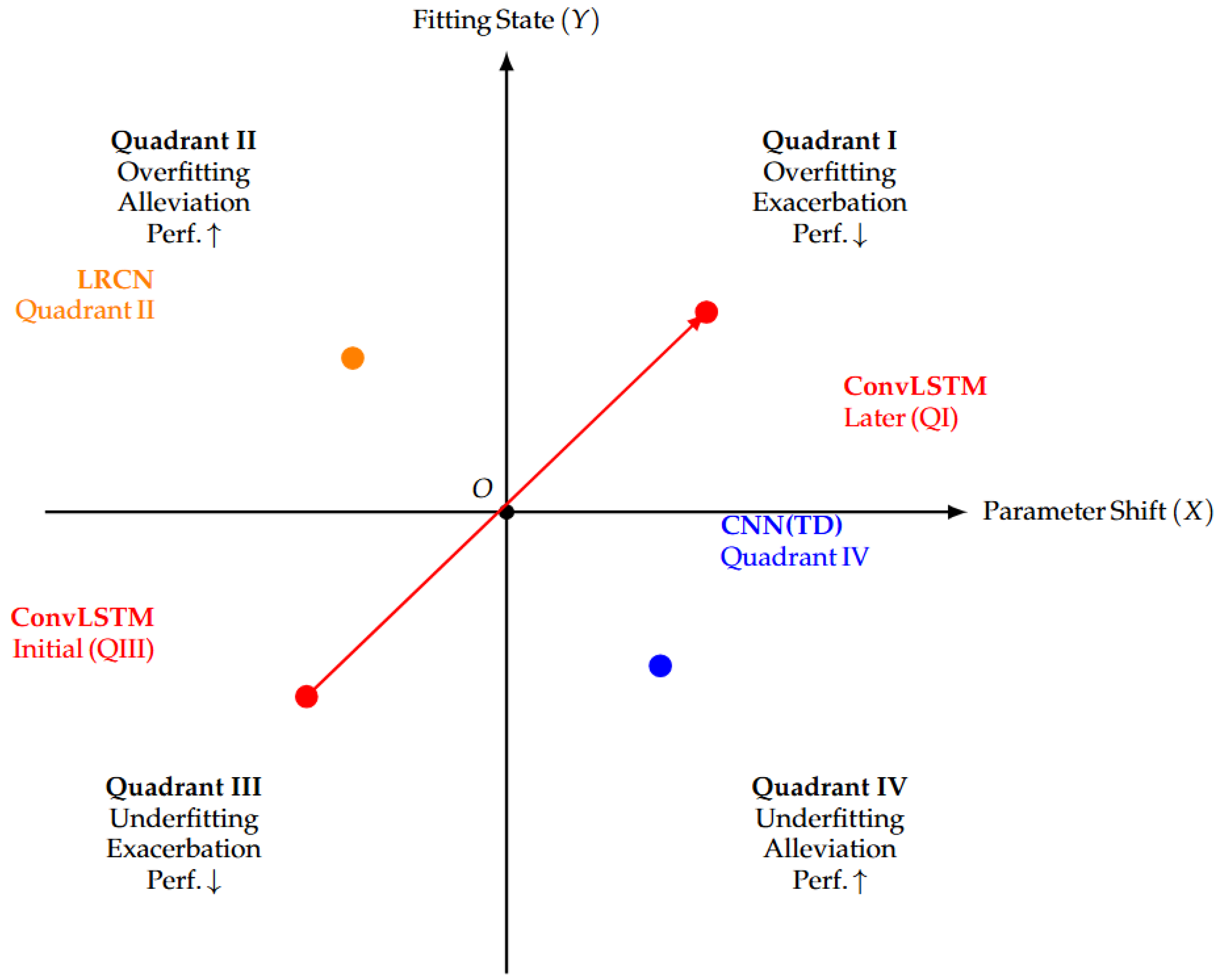
Furthermore, an in-depth analysis of model complexity versus performance was conducted using the Parameter Quantity Shifting–Fitting Performance (PQS-FP) [55] framework, a theoretical framework for analyzing the relationship between model complexity and performance based on how the parameter quantity affects the model fitting status. With the ideal parameter quantity O as the benchmark, the Y-axis represents the model’s fitting state (Y < 0 for underfitting, Y > 0 for overfitting), and the X-axis represents the direction of parameter change (X > 0 for increased parameters, X < 0 for decreased parameters. The framework divides the system into four quadrants: Quadrant I (overfitting exacerbation with performance decline), Quadrant II (overfitting alleviation with performance improvement), Quadrant III (underfitting exacerbation with performance decline), and Quadrant IV (underfitting alleviation with performance improvement). For the three models used in this work, the PQS-FP distribution over the quadrants is discussed further and shown in Figure 12.

LRCN (5.6 M parameters): This falls within Quadrant II (overfitting alleviation through regularization). While the VGG16 backbone introduces considerable parameters (X > 0), strategic application of a 0.5 dropout and freezing of the first 10 convolutional layers effectively mitigates the overfitting tendencies. The model maintains high accuracy (98.68%) but exhibits higher loss (0.0574) due to conservative softmax outputs from LSTM temporal smoothing, indicating slight residual overfitting (Y > 0, small) that is controlled through regularization.

CNN-TD (2.8M parameters): This is positioned in Quadrant IV (underfitting alleviation with performance improvement). The architecture achieves near-optimal parameterization relative to task complexity, effectively capturing spatial hierarchies through frame-wise convolutions without introducing excessive temporal coupling. The model’s stable convergence at 32 epochs with 98.68% accuracy and minimal loss (0.0236) indicates balanced parameter quantity near the ideal O, avoiding both underfitting (Y < 0) and overfitting (Y > 0) regimes.

ConvLSTM (10.2M parameters): This was initially positioned in Quadrant III (underfitting with excessive parameters relative to dataset size), then transitioned toward Quadrant I (overfitting exacerbation) as training progressed beyond 20 epochs. The model’s 3D convolutional operations introduce substantial parameter redundancy for short-duration actions, such as “pour” and “stir,” leading to the memorization of training-specific temporal variations rather than generalizable motion patterns. The validation loss increases to 0.2345 at epoch 40, confirming migration into an overfitting regime (Y > 0), despite the high parameter count (X > 0).

This PQS-FP analysis reveals that CNN-TD achieves optimal parameter–performance balance (Quadrant IV), LRCN manages over-parameterization through regularization (Quadrant II), while ConvLSTM suffers from parameter excess relative to the task requirements, leading to unstable fitting behavior (Quadrant III to I transition). The PQS–FP diagram as shown in Figure 12 validates our architectural choices by showing CNN-TD achieves optimal parameter–performance balance, LRCN effectively mitigates overfitting, and ConvLSTM’s instability arises from excessive parameters, supporting our comparative findings.

4.4. Discussion

This study evaluated the performance of three video classification models, LRCN, CNN-TD, and ConvLSTM, in the context of human–robot interaction, with the goal of understanding and interpreting human actions from video sequences. The models were tested on predicting two distinct robotic arm movements, representing daily-life actions captured on video. Our results demonstrate that these neural networks integrate feature extraction and prediction into a single end-to-end pipeline. While training these models generally requires a longer computational time compared to traditional algorithms, once trained, they can perform real-time predictions efficiently. Among the models tested, the CNN-TD achieved superior predictive performance compared to LRCN and ConvLSTM (CNN-3D), as it achieves almost the same accuracy, lower test loss (better generalization), and requires fewer epochs, making it more efficient for real-world deployment. Moreover, real-time inference was assessed on an Intel Core i7-5600 (6-core, 3.2 GHz) CPU, with 16 GB of RAM. The average throughputs were as follows: CNN-TD = 18 fps, LRCN = 13 fps, ConvLSTM = 10 fps. All real-time inference experiments were conducted on an Ubuntu 20.04 LTS (64-bit). The software environment consisted of Python 3.9, TensorFlow 2.10 (CPU build), Keras 2.10, NumPy 1.23, and OpenCV 4.x. TensorFlow executed the models in tf.function graph mode, and inference was performed with a batch size of 1, using pre-loaded sequences to avoid I/O overhead. Each FPS value represents the mean over 30 repeated runs. This detailed specification ensures reproducibility and enables consistent comparison with other real-time HAR systems. We define real-time capability as greater than or equal to 15 frames per second (fps), distinguishing between the training-time convergence speed and inference-time throughput. The time-distributed CNN exhibits slightly higher CPU usage (3.0–3.5 GB) due to frame-wise parallel convolutional execution; however, it compensates with faster convergence and lower total runtime. The LRCN model maintains moderate CPU load (2.3–2.7 GB) owing to sequential LSTM processing, while the ConvLSTM (2.5–3.2 GB) balances between spatial convolution and temporal recurrence. These results affirm that CNN-TD achieves the most favorable trade-off between computational efficiency and accuracy, making it optimal for real-time human–robot interaction applications. CNN(TD) exhibits higher CPU usage (3.0–3.5 GB) due to its frame-level parallel convolutions, which are executed through the time-distributed layer, resulting in increased memory overhead but yielding faster throughput (18 fps). Thus, “real-time performance” refers to the inference speed, not the memory footprint. To ensure suitability for embedded deployment, quantization, pruning, and frame-buffer optimization will be applied to reduce memory usage below 2 GB without affecting inference speed. The manuscript will also clarify the distinction between training-time convergence (fast learning) and inference-time real-time performance (≥15 fps) to prevent conceptual confusion. The detailed explanation of the experimental settings is shown in

Table 4. Experimental settings used in NovAc-DL experiments.

Category	Specification
Hardware Configuration	CPU: Intel Core i7-5600 (6 cores @ 3.2 GHz); RAM: 16 GB;
	GPU: fixed 16 GB configuration (used across all models).
Software Environment	Python 3.x; TensorFlow (TF–Keras backend); Keras layers (Conv2D, MaxPooling2D,
	LSTM, ConvLSTM2D, TimeDistributed, Dropout); OpenCV [56] for video preprocessing.
Dataset Parameters	Total videos: 2000 (Pour: 1000; Stir: 1000 after balancing);
	Frame size: 224 × 224 pixels; FPS: 30; sequence length: 30 frames/video;
	dataset split: 64% training, 16% validation, 20% testing.
Common Training Settings	Optimizer: Adam [51]; learning rate: $1\times {10}^{-4}$; ${\beta }_1=0.9$, ${\beta }_2=0.999$, $ϵ={10}^{-7}$;
	batch size: 16; epochs: 40 (CNN-TD early-stopped at 32);
	loss function: categorical cross-entropy.
LRCN Configuration	Backbone: VGG16 pre-trained on ImageNet (first 10 conv layers frozen, last 5 fine-tuned);
	LSTM: 256 units; dropout: 0.5; dense: 64 units + softmax (3 classes);
	ensemble: 5 seeds (0, 7, 21, 37, 45) with majority voting.
CNN-TD Configuration	Conv2D filters: 64, 128, 256 (kernel size 3 × 3); maxpooling: 2 × 2;
	dropout: 0.2; TimeDistributed wrapper applied to CNN layers.
ConvLSTM Configuration	ConvLSTM2D: 64 filters, 3 × 3 kernel; ReLU activation; dropout: 0.1;
	preserved spatial–temporal structure via 3D convolutional gating.
Inference Metrics	Real-time throughput: CNN-TD = 18 FPS; LRCN = 13 FPS; ConvLSTM = 10 FPS;
	CPU memory usage: LRCN = 2.3–2.7 GB; CNN-TD = 3.0–3.5 GB; ConvLSTM = 2.5–3.2 GB.

.

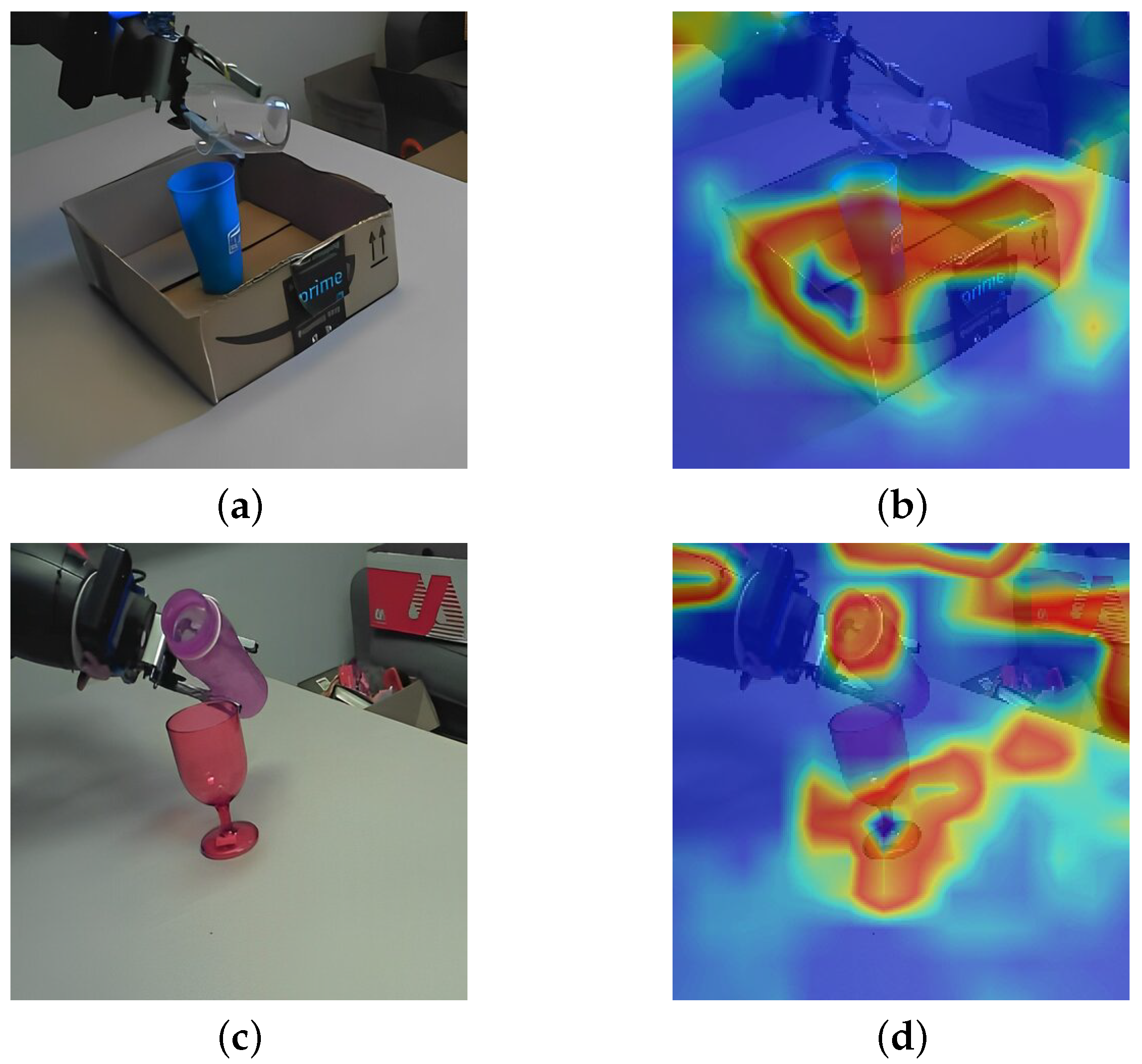
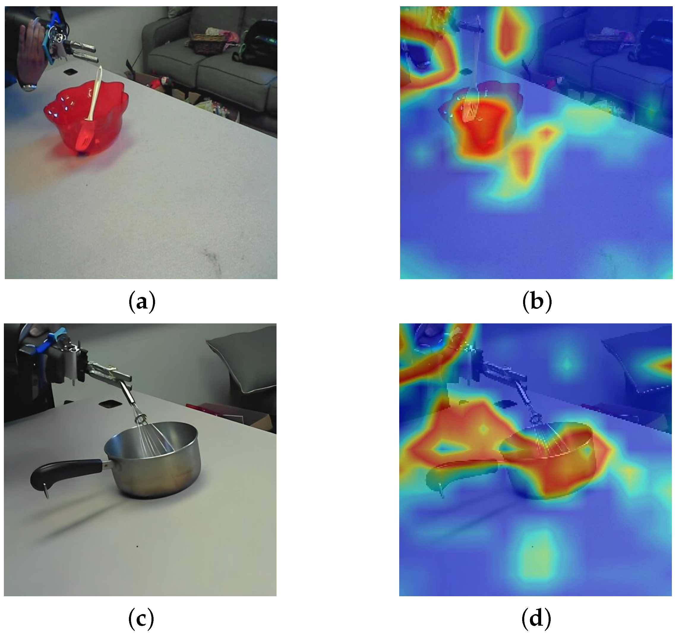
Figure 13 demonstrates the class-activation mapping for the “Pour” activity, where Grad–CAM [57] highlights the regions that contribute most to classification. The red-to-yellow intensity zones align with the region of interaction between the container and target surface, precisely where liquid transfer motion occurs. This confirms that the CNN focuses on contextually relevant spatial cues rather than background pixels. The visualization further validates the model’s transparency and interpretability, showing that learned attention corresponds to semantically meaningful features in the frame sequence.

Grad-CAM was applied to the final Conv2D block of CNN-TD preceding the global average pooling layer. Gradients of the class-specific score were back-propagated using the Keras GradientTape API. The resulting heatmaps were normalized (0–1) and visualized with a 0.4 threshold to highlight action-salient regions. In Figure 14, the Grad–CAM heatmaps highlight attention along the spoon trajectory and bowl interior, depicting the cyclic motion pattern characteristic of stirring. Compared to “pour,” the attention distribution here is more circular and temporally repetitive, emphasizing the model’s ability to capture fine-grained motion semantics. This distinction demonstrates that the network learns motion-based representations rather than relying solely on object presence, thus enabling robust differentiation of visually similar gestures.

The findings hold substantial potential for industrial automation, particularly in monitoring and optimizing packaging processes. By leveraging these predictive capabilities, industries can enhance operational efficiency, improve productivity, and ensure precise and seamless handling of goods, thereby advancing the integration of intelligent robotic systems into practical workflows.

The selection of CNN- and LSTM-based architectures in this work stems from the spatiotemporal characteristics of the pour and stir activities, which require the model to capture both localized spatial cues (edge orientation, container alignment, hand–object interaction) and evolving temporal patterns across frames. Each network was therefore evaluated based on how effectively its design captures these dual characteristics. The CNN-TD demonstrated the strongest performance, achieving 98.68% accuracy with minimal validation loss, primarily due to its frame-wise convolutional parallelism, which efficiently extracts discriminative spatial features while reducing redundancy across consecutive frames. The LRCN model achieved stable but slower convergence because its recurrent gates must sequentially process longer frame sequences, whereas the ConvLSTM experienced a decline in accuracy owing to the computational overhead imposed by 3D convolutions. These differences confirm that architectural efficiency directly influences convergence behavior, generalization capability, and suitability for real-time deployment.

Among the evaluated models, CNN-TD proved to be the most effective, offering the best balance between accuracy and computational cost (3.0–3.5 GB CPU usage, convergence within 32 epochs), making it ideal for practical robotic applications. Grad-CAM visualizations further verified that the model consistently attends to motion-relevant regions, reinforcing its interpretability and reliability. While transformer-based architectures are powerful for long-range temporal reasoning, they typically demand large training datasets and significantly higher computational resources. Given the moderate size of our curated dataset (2000 videos, balanced across classes) and the real-time constraints of robotic manipulation tasks, the CNN–LSTM family provided an optimal trade-off: strong spatiotemporal modeling capacity, fast convergence, and robust action discrimination for activities that differ more in motion dynamics than in appearance.

5. Conclusions

This study successfully developed and evaluated a deep learning-based framework, NovAc-DL, for recognizing human-like actions such as “pour” and “stir” in real-time environments. By employing three spatial–temporal architectures, i.e., LRCN, CNN-TD, and ConvLSTM, the research has demonstrated how temporal dependencies and spatial features can be effectively integrated for precise activity recognition. Grad-CAM was used to interpret model predictions and localize motion-specific regions corresponding to “pour” and “stir” gestures. Overall, the proposed approach has proven to be efficient, generalizable, and computationally feasible, offering a strong foundation for the future integration of intelligent activity recognition in industrial automation, healthcare monitoring, and collaborative robotics. Future research will extend NovAc-DL by expanding the dataset to multiple composite actions and cross-subject variations, exploring transformer-based temporal encoders for longer dependencies, applying pruning and quantization for embedded deployment, and integrating multimodal inputs such as IMU and depth sensors for context-aware robotic perception. In the manuscript, equal accuracy but different losses for CNN-TD and LRCN are reported. The LRCN incorporates an LSTM layer over VGG16-extracted features, which intentionally smooths temporal predictions. This reduces the softmax confidence (making the model more conservative), thereby increasing loss while keeping the accuracy unchanged.

References

1. LeCun, Y.; Bengio, Y.; Hinton, G. Deep learning. Nature 2015, 521, 436–444. [Google Scholar] [CrossRef] [PubMed]
2. Hinton, G.E.; Osindero, S.; Teh, Y.W. A fast learning algorithm for deep belief nets. Neural Comput. 2006, 18, 1527–1554. [Google Scholar] [CrossRef] [PubMed]
3. Karpathy, A.; Toderici, G.; Shetty, S.; Leung, T.; Sukthankar, R.; Fei-Fei, L. Large-scale video classification with convolutional neural networks. In Proceedings of the IEEE Conference on Computer Vision and Pattern Recognition (CVPR 2014), Columbus, OH, USA, 23–28 June 2014; pp. 1725–1732. [Google Scholar]
4. Simonyan, K.; Zisserman, A. Two-stream convolutional networks for action recognition in videos. In Proceedings of the Advances in Neural Information Processing Systems (NIPS 2014), Montreal, QC, Canada, 8–13 December 2014; pp. 568–576. [Google Scholar]
5. Mehrish, A.; Majumder, N.; Bharadwaj, R.; Mihalcea, R.; Poria, S. A review of deep learning techniques for speech processing. Inf. Fusion 2023, 99, 101869. [Google Scholar] [CrossRef]
6. Do, T.T.T.; Huynh, Q.T.; Kim, K.; Nguyen, V.Q. A Survey on Video Big Data Analytics: Architecture, Technologies, and Open Research Challenges. Appl. Sci. 2025, 15, 8089. [Google Scholar] [CrossRef]
7. Liu, X.; Xiang, X.; Li, Z.; Wang, Y.; Li, Z.; Liu, Z.; Zhang, W.; Ye, W.; Zhang, J. A survey of ai-generated video evaluation. arXiv 2024, arXiv:2410.19884. [Google Scholar] [CrossRef]
8. Kansal, S.; Jha, S.; Samal, P. DL-DARE: Deep learning-based different activity recognition for the human–robot interaction environment. Neural Comput. Appl. 2023, 35, 12029–12037. [Google Scholar] [CrossRef]
9. Zhu, S.; Chen, W.; Liu, F.; Zhang, X.; Han, X. Human Activity Recognition Based on a Modified Capsule Network. Mob. Inf. Syst. 2023, 2023, 8273546. [Google Scholar] [CrossRef]
10. Uddin, M.A.; Talukder, M.A.; Uzzaman, M.S.; Debnath, C.; Chanda, M.; Paul, S.; Islam, M.M.; Khraisat, A.; Alazab, A.; Aryal, S. Deep learning-based human activity recognition using CNN, ConvLSTM, and LRCN. Int. J. Cogn. Comput. Eng. 2024, 5, 259–268. [Google Scholar] [CrossRef]
11. Donahue, J.; Hendricks, L.A.; Guadarrama, S.; Rohrbach, M.; Venugopalan, S.; Saenko, K.; Darrell, T. Long-term Recurrent Convolutional Networks for Visual Recognition and Description. In Proceedings of the IEEE Conference on Computer Vision and Pattern Recognition (CVPR), Boston, MA, USA, 7–12 June 2015; pp. 2625–2634. [Google Scholar]
12. Ljajic, A. Deep Learning-Based Body Action Classification and Ergonomic Assessment. Ph.D. Thesis, Technische Universität Wien, Vienna, Austria, 2024. [Google Scholar]
13. Lee, J.W.; Kang, H.S. Three-stage deep learning framework for video surveillance. Appl. Sci. 2024, 14, 408. [Google Scholar] [CrossRef]
14. Yoshidomi, T.; Kume, S.; Aizawa, H.; Furui, A. Classification of Carotid Plaque with Jellyfish Sign Through Convolutional and Recurrent Neural Networks Utilizing Plaque Surface Edges. arXiv 2024, arXiv:2406.18919. [Google Scholar] [CrossRef]
15. Arulalan, V. Deep Learning Based Methods for Improving Object Detection, Classification and Tracking in Video Surveillance. Ph.D. Thesis, Anna University, Chennai, India, 2023. [Google Scholar]
16. Tabassum, I. A Hybrid Deep-Learning Approach for Multi-Class Cyberbullying Classification of Cyberbullying Using Social Medias’ Multi-Modal Data. Master’s Thesis, University of South-Eastern Norway, Notodden, Norway, 2024. [Google Scholar]
17. Das, A.; Mistry, D.; Kamal, R.; Ganguly, S.; Chakraborty, S. Facemask and Hand Gloves Detection Using Hybrid Deep Learning Model. In Smart Medical Imaging for Diagnosis and Treatment Planning; Chapman and Hall/CRC: Boca Raton, FL, USA, 2025; pp. 176–198. [Google Scholar]
18. Lei, J.; Sun, W.; Fang, Y.; Ye, N.; Yang, S.; Wu, J. A Model for Detecting Abnormal Elevator Passenger Behavior Based on Video Classification. Electronics 2024, 13, 2472. [Google Scholar] [CrossRef]
19. Rahayu, E.S.; Yuniarno, E.M.; Purnama, I.K.E.; Purnomo, M.H. Human activity classification using deep learning based on 3D motion feature. Mach. Learn. Appl. 2023, 12, 100461. [Google Scholar] [CrossRef]
20. Helmi, A.M.; Al-qaness, M.A.; Dahou, A.; Abd Elaziz, M. Human activity recognition using marine predators algorithm with deep learning. Future Gener. Comput. Syst. 2023, 142, 340–350. [Google Scholar] [CrossRef]
21. Islam, M.M.; Nooruddin, S.; Karray, F.; Muhammad, G. Multi-level feature fusion for multimodal human activity recognition in Internet of Healthcare Things. Inf. Fusion 2023, 94, 17–31. [Google Scholar] [CrossRef]
22. Hurtado, S.; García-Nieto, J.; Popov, A.; Navas-Delgado, I. Human Activity Recognition From Sensorised Patient’s Data in Healthcare: A Streaming Deep Learning-Based Approach. Int. J. Interact. Multimed. Artif. Intell. 2023, 8, 23–37. [Google Scholar] [CrossRef]
23. Sharma, V.; Gupta, M.; Kumar, A.; Mishra, D. Video processing using deep learning techniques: A systematic literature review. IEEE Access 2021, 9, 139489–139507. [Google Scholar] [CrossRef]
24. Savran Kızıltepe, R.; Gan, J.Q.; Escobar, J.J. A novel keyframe extraction method for video classification using deep neural networks. Neural Comput. Appl. 2021, 35, 24513–24524. [Google Scholar] [CrossRef]
25. Naik, K.J.; Soni, A. Video classification using 3D convolutional neural network. In Advancements in Security and Privacy Initiatives for Multimedia Images; IGI Global: Palmdale, PA, USA, 2021; pp. 1–18. [Google Scholar]
26. Xu, Y. A sports training video classification model based on deep learning. Sci. Program. 2021, 2021, 7252896. [Google Scholar] [CrossRef]
27. Pentyala, S.; Dowsley, R.; De Cock, M. Privacy-preserving video classification with convolutional neural networks. In Proceedings of the International Conference on Machine Learning, PMLR, Virtual, 18–24 July 2021; pp. 8487–8499. [Google Scholar]
28. Rehman, A.; Belhaouari, S.B. Deep Learning for Video Classification: A Review. TechRxiv 2021, 1, 20–41. [Google Scholar]
29. Howard, J.P.; Tan, J.; Shun-Shin, M.J.; Mahdi, D.; Nowbar, A.N.; Arnold, A.D.; Ahmad, Y.; McCartney, P.; Zolgharni, M.; Linton, N.W.; et al. Improving ultrasound video classification: An evaluation of novel deep learning methods in echocardiography. J. Med. Artif. Intell. 2020, 3, 4. [Google Scholar] [CrossRef]
30. Wang, L.; Xiong, Y.; Wang, Z.; Qiao, Y.; Lin, D.; Tang, X.; Gool, L.V. Temporal Segment Networks: Towards Good Practices for Deep Action Recognition. In Proceedings of the European Conference on Computer Vision, Amsterdam, The Netherlands, 11–14 October 2016; Lecture Notes in Computer Science. Springer: Cham, Switzerland, 2016; Volume 9912, pp. 20–36. [Google Scholar] [CrossRef]
31. Wang, L.; Zhang, H.; Yuan, G. Big data and deep learning-based video classification model for sports. Wirel. Commun. Mob. Comput. 2021, 2021, 1140611. [Google Scholar] [CrossRef]
32. Verma, T.; Dubey, S. Prediction of diseased rice plant using video processing and LSTM-simple recurrent neural network with comparative study. Multimed. Tools Appl. 2021, 80, 29267–29298. [Google Scholar] [CrossRef]
33. Zhang, Y.; Kwong, S.; Xu, L.; Zhao, T. Advances in Deep-Learning-Based Sensing, Imaging, and Video Processing. Sensors 2022, 22, 6192. [Google Scholar] [CrossRef]
34. Uchiyama, T.; Sogi, N.; Niinuma, K.; Fukui, K. Visually explaining 3D-CNN predictions for video classification with an adaptive occlusion sensitivity analysis. In Proceedings of the IEEE/CVF Winter Conference on Applications of Computer Vision, Waikoloa, HI, USA, 2–7 January 2023; pp. 1513–1522. [Google Scholar]
35. Shea, D.E.; Kulhare, S.; Millin, R.; Laverriere, Z.; Mehanian, C.; Delahunt, C.B.; Banik, D.; Zheng, X.; Zhu, M.; Ji, Y.; et al. Deep Learning Video Classification of Lung Ultrasound Features Associated with Pneumonia. In Proceedings of the IEEE/CVF Conference on Computer Vision and Pattern Recognition, Vancouver, BC, Canada, 17–24 June 2023; pp. 3102–3111. [Google Scholar]
36. Ramesh, M.; Mahesh, K. Sports Video Classification Framework Using Enhanced Threshold-Based Keyframe Selection Algorithm and Customized CNN on UCF101 and Sports1-M Dataset. Comput. Intell. Neurosci. 2022, 2022, 3218431. [Google Scholar] [CrossRef]
37. Tang, H.; Ding, L.; Wu, S.; Ren, B.; Sebe, N.; Rota, P. Deep unsupervised key frame extraction for efficient video classification. ACM Trans. Multimed. Comput. Commun. Appl. 2023, 19, 1–17. [Google Scholar] [CrossRef]
38. Agnusdei, G.P.; Elia, V.; Gnoni, M.G. A classification proposal of digital twin applications in the safety domain. Comput. Ind. Eng. 2021, 154, 107137. [Google Scholar] [CrossRef]
39. Lee, J.; Cameron, I.; Hassall, M. Improving process safety: What roles for Digitalization and Industry 4.0? Process Saf. Environ. Prot. 2019, 132, 325–339. [Google Scholar] [CrossRef]
40. Bakshi, R. Hand hygiene video classification based on deep learning. arXiv 2021, arXiv:2108.08127. [Google Scholar] [CrossRef]
41. Chelliah, B.J.; Harshitha, K.; Pandey, S. Adaptive and effective spatio-temporal modelling for offensive video classification using deep neural network. Int. J. Intell. Eng. Inform. 2023, 11, 19–34. [Google Scholar] [CrossRef]
42. Li, H.; Cryer, S.; Acharya, L.; Raymond, J. Video and image classification using atomisation spray image patterns and deep learning. Biosyst. Eng. 2020, 200, 13–22. [Google Scholar]
43. Sabzi, S.; Pourdarbani, R.; Kalantari, D.; Panagopoulos, T. Designing a fruit identification algorithm in orchard conditions to develop robots using video processing and majority voting based on hybrid artificial neural network. Appl. Sci. 2020, 10, 383. [Google Scholar] [CrossRef]
44. Li, G.Y.; Chen, L.; Zahiri, M.; Balaraju, N.; Patil, S.; Mehanian, C.; Gregory, C.; Gregory, K.; Raju, B.; Kruecker, J.; et al. Weakly Semi-Supervised Detector-Based Video Classification with Temporal Context for Lung Ultrasound. In Proceedings of the IEEE/CVF International Conference on Computer Vision, Paris, France, 1–6 October 2023; pp. 2483–2492. [Google Scholar]
45. Qian, R.; Li, Y.; Xu, Z.; Yang, M.H.; Belongie, S.; Cui, Y. Multimodal open-vocabulary video classification via pre-trained vision and language models. arXiv 2022, arXiv:2207.07646. [Google Scholar]
46. Kansal, S.; Kansal, P. Robotic Hand Pour & Stir Video Dataset. 2023. Available online: https://www.kaggle.com/datasets/8baa9574ce5ae310af601d342765670b61246e37140a6d190270f4601424a058 (accessed on 9 September 2025).
47. Soomro, K.; Zamir, A.R.; Shah, M. UCF101: A dataset of 101 human actions classes from videos in the wild. arXiv 2012, arXiv:1212.0402. [Google Scholar] [CrossRef]
48. Kuehne, H.; Jhuang, H.; Garrote, E.; Poggio, T.; Serre, T. HMDB: A large video database for human motion recognition. In Proceedings of the 2011 International Conference on Computer Vision (ICCV 2011), Barcelona, Spain, 6–13 November 2011; pp. 2556–2563. [Google Scholar]
49. Simonyan, K.; Zisserman, A. Very Deep Convolutional Networks for Large-Scale Image Recognition. In Proceedings of the International Conference on Learning Representations (ICLR), San Diego, CA, USA, 7–9 May 2015. [Google Scholar]
50. Nair, V.; Hinton, G.E. Rectified Linear Units Improve Restricted Boltzmann Machines. In Proceedings of the 27th International Conference on Machine Learning (ICML), Haifa, Israel, 21–24 June 2010; pp. 807–814. [Google Scholar]
51. Kingma, D.P.; Ba, J. Adam: A Method for Stochastic Optimization. In Proceedings of the International Conference on Learning Representations (ICLR), San Diego, CA, USA, 7–9 May 2015. [Google Scholar]
52. Shi, X.; Chen, Z.; Wang, H.; Yeung, D.Y.; Wong, W.K.; Woo, W.C. Convolutional LSTM network: A machine learning approach for precipitation nowcasting. In Proceedings of the Advances in Neural Information Processing Systems (NIPS 2015), Montreal, QC, Canada, 7–12 December 201; pp. 802–810.
53. Pedregosa, F.; Varoquaux, G.; Gramfort, A.; Michel, V.; Thirion, B.; Grisel, O.; Blondel, M.; Prettenhofer, P.; Weiss, R.; Dubourg, V.; et al. Scikit-learn: Machine Learning in Python. J. Mach. Learn. Res. 2011, 12, 2825–2830. [Google Scholar]
54. Xiang, Q.; Wang, X.; Lei, L.; Song, Y. Dynamic bound adaptive gradient methods with belief in observed gradients. Pattern Recognit. 2025, 168, 111819. [Google Scholar] [CrossRef]
55. Xiang, Q.; Wang, X.; Lai, J.; Lei, L.; Song, Y.; He, J.; Li, R. Quadruplet depth-wise separable fusion convolution neural network for ballistic target recognition with limited samples. Expert Syst. Appl. 2024, 235, 121182. [Google Scholar] [CrossRef]
56. Bradski, G. The OpenCV Library. Dr. Dobb’S J. Softw. Tools 2000. Available online: https://jacobfilipp.com/DrDobbs/articles/DDJ/2000/0011/0011k/0011k.htm?utm_source=chatgpt.com (accessed on 15 September 2025).
57. Selvaraju, R.R.; Cogswell, M.; Das, A.; Vedantam, R.; Parikh, D.; Batra, D. Grad-CAM: Visual explanations from deep networks via gradient-based localization. In Proceedings of the IEEE International Conference on Computer Vision (ICCV), Venice, Italy, 22–29 October; pp. 618–626.
Figure 1. A concept of video data.
Bdcc 10 00011 g001
Figure 2. Representative frames for the pour class showing the action phases: (a) initial setup (glass and pan on table), (b) alignment of the source container over the target, (c) onset of tilt, (d) active transfer of liquid, and (e) completion with return to neutral.
Bdcc 10 00011 g002
Figure 3. Representative frames for the stir class highlighting cyclic motion: (a) initial setup (bowl + spoon), (b) tool lift via robotic arm, (c) motion onset within the bowl, (d) sustained cyclic stirring, (e) motion decay/slowdown.
Bdcc 10 00011 g003
Figure 4. Overview of the LRCN model used to detect suspicious activity.
Bdcc 10 00011 g004
Figure 5. LRCN model.
Bdcc 10 00011 g005
Figure 6. The convolutional input and output.
Bdcc 10 00011 g006
Figure 7. ConvLSTM model.
Bdcc 10 00011 g007
Figure 8. Individual training dynamics of CNN-TD model: (a) accuracy progression and (b) loss reduction over epochs.
Bdcc 10 00011 g008
Figure 9. Individual training dynamics of LRCN model: (a) accuracy progression and (b) loss reduction over epochs.
Bdcc 10 00011 g009
Figure 10. Individual training dynamics of ConvLSTM model: (a) accuracy progression and (b) loss reduction over epochs.
Bdcc 10 00011 g010
Figure 11. Comparative training and validation accuracy curves for LRCN, CNN-TD, and ConvLSTM models. The CNN-TD achieves the fastest and smoothest convergence (32 epochs), while LRCN converges steadily (40 epochs), and ConvLSTM exhibits oscillations due to its higher 3D convolutional complexity. This comparative visualization illustrates the differences in convergence speed, stability, and generalization across various architectures.
Bdcc 10 00011 g011
Figure 12. PQS–FP framework illustrating the relationship between parameter quantity (X-axis) and fitting state (Y-axis). The ideal parameter quantity is indicated by O at the origin. CNN-TD lies in Quadrant IV (underfitting alleviation with performance improvement) and LRCN in Quadrant II (overfitting alleviation via regularization), while ConvLSTM transitions from Quadrant III (underfitting with excessive parameters) to Quadrant I (overfitting exacerbation).
Bdcc 10 00011 g012
Figure 13. Grad-CAM visualization for pour. (a,c): original frame; (b,d): overlay of the CNN-TD activation map (normalized 0–1; same colormap/alpha across figures; colorbar shown). High-saliency regions (yellow–red) concentrate at the container–target interface during liquid transfer, indicating that the model attends to motion-relevant pixels rather than background.
Bdcc 10 00011 g013
Figure 14. Grad-CAM visualization for stir. (a,c): original frame; (b,d): overlay from the CNN-TD (normalized 0–1; consistent colormap/alpha; colorbar shown). High-saliency regions (yellow–red) traces the spoon trajectory and bowl interior, forming a circular temporally repetitive pattern characteristic of stirring.
Bdcc 10 00011 g014