Determination of a Numerical Surge Limit by Means of an Enhanced Greitzer Compressor Model ^†

Abstract

The surge limit of centrifugal compressors is a key parameter in the design process of modern turbochargers. Numerical methods like steady-state simulations are state-of-the-art methods for predicting the performance of the centrifugal compressor. In contrast to that, the determination of the surge limit with any numerical method is still an unsolved challenge. Since the extensive work of Greitzer and many other researchers in this field, it is well-known that surge is a system-dependent phenomenon. In the case of steady-state simulations, the simulation domain is chosen to be as small as possible due to the numerical cost. This simply implies that there is no system information included in the numerical model. Therefore, it is not possible to determine any system-dependent surge limit with today’s applied numerical methods. To overcome this issue, an enhanced Greitzer surge model, which has been developed at Tu Darmstadt, should act as a link between the simulation and the system in which the compressor will be operated. The focus of this paper will rather be on the methodology of determining the surge limit by means of numerical data than on the surge model itself. The methodology will be validated by experimental data of different systems.

1. Introduction

Through the past years, the ratio of boosting internal combustion engines (ICE) has been increased gradually and the dynamic response behaviour has been improved significantly. This has been achieved by combining multiple sizes of turbochargers on the one hand and intelligent, closed-loop controls on the other hand. Even if the complexity has increased over the years, the basic principle of boosting an ICE is still the same and is depicted by a basic assembly diagram of a turbocharged ICE in Figure 1a.

From the basic assembly diagram in Figure 1a, an important thing can be seen. The engine intake flow path consists of an air filter, a compressor and an intercooler, as well as a certain amount of piping between all of these components. The piping depends especially on the engine architecture and varies between different applications. All of the components upstream of the compressor inlet obviously induce a certain pressure loss, depending on the components’ design as well as the flow rate. The components downstream of the compressor primarily result in a certain plenum size. So, if the same compressor wheel is used for different engines or engine configurations, the compressor wheel is operated in different systems. The so-called system can be generalized by throttles (pressure loss components), the compressor (pressure rise component) and volumes. Based on this, the flow diagram from Figure 1a can be transferred into the diagram in Figure 1b. Every subcomponent along the flowpath can then be mathematically modeled by its own characteristic.

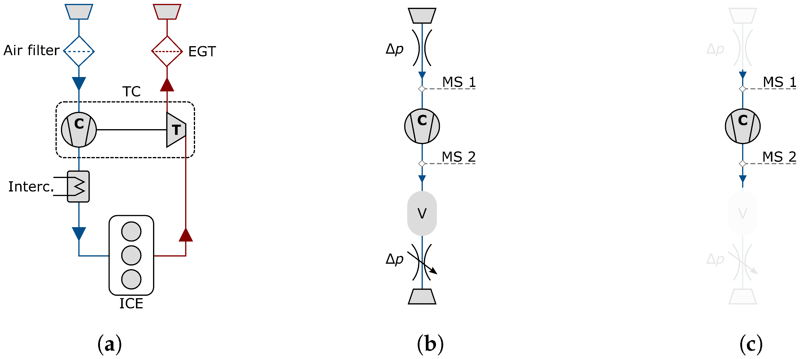
1.1. The Surge Limit as a Function of the System

Since the fundamental publications of Greitzer in the 1970s for axial compressors [1,2], it is well-known that surge is a system-dependent phenomenon. At this point, it is important to say that surge, in this case, needs to be distinguished from small-scale stall phenomena that can often be seen for axial compressors. Surge is a global phenomenon including the piping upstream and downstream of the compressor. Greitzer showed that the exit plenum has a significant influence on the location of the surge limit. The dependency on the outlet plenum size can be estimated by the well-known B-parameter (Equation (1)).

$$B=\frac{u}{2a}\sqrt{\frac{V_{\mathrm{P}}}{A_{\mathrm{C}}{L}_{\mathrm{C}}}}$$

(1)

In this equation, u is the compressor speed, a the speed of sound, $V_{\mathrm{P}}$ the compressor exit plenum size and $A_{\mathrm{C}}$ and $L_{\mathrm{C}}$ are the compressor’s equivalent cross-sectional area and length. Based on linear system analysis and for a system with a very large plenum ($B\to \infty$), surge occurs at the peak pressure ratio, when the slope of the compressor characteristic $c^{\prime }=d\Delta p_{\mathrm{s},\mathrm{C}}/d\mathrm{\Phi }$ becomes positive. The compressor characteristic is, thus, an important parameter. Some years later in the 1990s, Fink et al. [3] applied the findings on centrifugal compressors and confirmed the same as for axial compressors. With a small B system, it was possible to operate the compressor to a mass flow rate of almost zero. In the years after, a few researchers were improving and applying the initial modeling approach and published the results for the scientific community [4,5,6,7,8,9,10]. Common to all of them is the fact that the compressor characteristic is modeled by a functional relationship. Formulating this relationship in a generalized form to fit all kinds of compressor wheels is a costly undertaking. What all of these showed by the mathematical formulation, as well as the associated experiments, is the influence of the system on the surge limit.

1.2. Numerical Modeling and the Challenge with the Surge Limit

In the current investigation, the compressor characteristic is determined by means of numerical simulations. The setup of these simulations uses a steady-state approach, since the performance data over a wide range of mass flow rates and compressor speeds are required. The details of the numerical setup have been published by Dielenschneider et al. [11] and will therefore not be mentioned again from this point. A more important detail is the simulated flow domain, which should be repeated and explained at this point by Figure 1c. The numerically simulated flow path differs significantly from the experimental setup (cf. Figure 1b,c). The numerical domain starts at the measurement section upstream of the compressor inlet (MS 1) and ends at the measurement section downstream of the compressor (MS 2). It basically consists of the compressor stage only. There is no additional piping or any throttle up- and downstream of the compressor. By default, a constant total pressure of 100,000 Pa is defined as the inlet boundary condition. A certain operating point is set by defining a constant mass flow rate as the outlet boundary condition. As a criterion for surge, the numerical convergence is often used. As the numerical investigations of the authors showed, it is possible to achieve converged results in a very wide mass flow range. However, considering that the numerical model does not include the system information, the numerical convergence is not a good criterion to determine the surge limit of a certain application.

In the literature, many very extensive, numerical investigations on surge in centrifugal compressors can be found. Since steady-state simulations cannot capture the transient flow dynamics of surge, many investigations use complex transient simulation methods like Large Eddy Simulations (LES) [12,13,14]. The results for a certain low mass flow rate show the pulsating nature of surge in the pressure and pressure ratio signals. These publications have their focus on the flow phenomena leading to surge, which they explain in a detailed manner. But, they all neglect the influence of the system on the surge initiation. Additionally, these kinds of simulations are very computationally expensive and, thus, are not options in an industrial environment. A second category of approaches uses steady-state simulation data and tries to link a physical parameter to the existence of surge, indicated by experiments which have also been conducted [15,16]. Some examples are the temperature at the leading edge (indicator for recirculation flow), the entropy production in the compressor wheel tip region (indicator for the tip gap vortex) or the velocity (indicator for flow reversal), which have been selected as physical parameters for surge detection. Just like the first category (highly detailed transient simulations), these publications also neglect the system influence. The third category is not exactly comparable since it does not use CFD-data for the compressor wheel. It should be pointed out at this point, nevertheless. The procedure of this category uses experimental data for the compressor wheel and a commercially available, quasi 1D engine simulation code to simulate the dynamic system behaviour [17]. Within this model, all of the ducting around the compressor is considered. The compressor performance is provided by a 0D look-up table and is extrapolated to choke, zero mass flow rate and reverse flow. This approach enables the simulation of system-dependent surge. The disadvantage of this approach is the extrapolation of speedlines. As a conclusion, it can be said that as far as the authors know, the determination of the surge limit by means of steady-state CFD-simulations with respect to a certain system is still an unsolved challenge (cf. [18]).

2. Determination of the Surge Limit

The basic idea for determining a system-dependent surge limit is to split the compressor wheel and the system and bring them together again in a second step. The compressor wheel performance is gained by steady-state CFD-simulations. On the other hand, the system is represented by an analytical model based on the Greitzer approach. The initial approach has been extended in-house at Tu Darmstadt to consider the compressor inlet system. Further details about the development and the underlying equations have been published by Bühler et al. in [19,20].

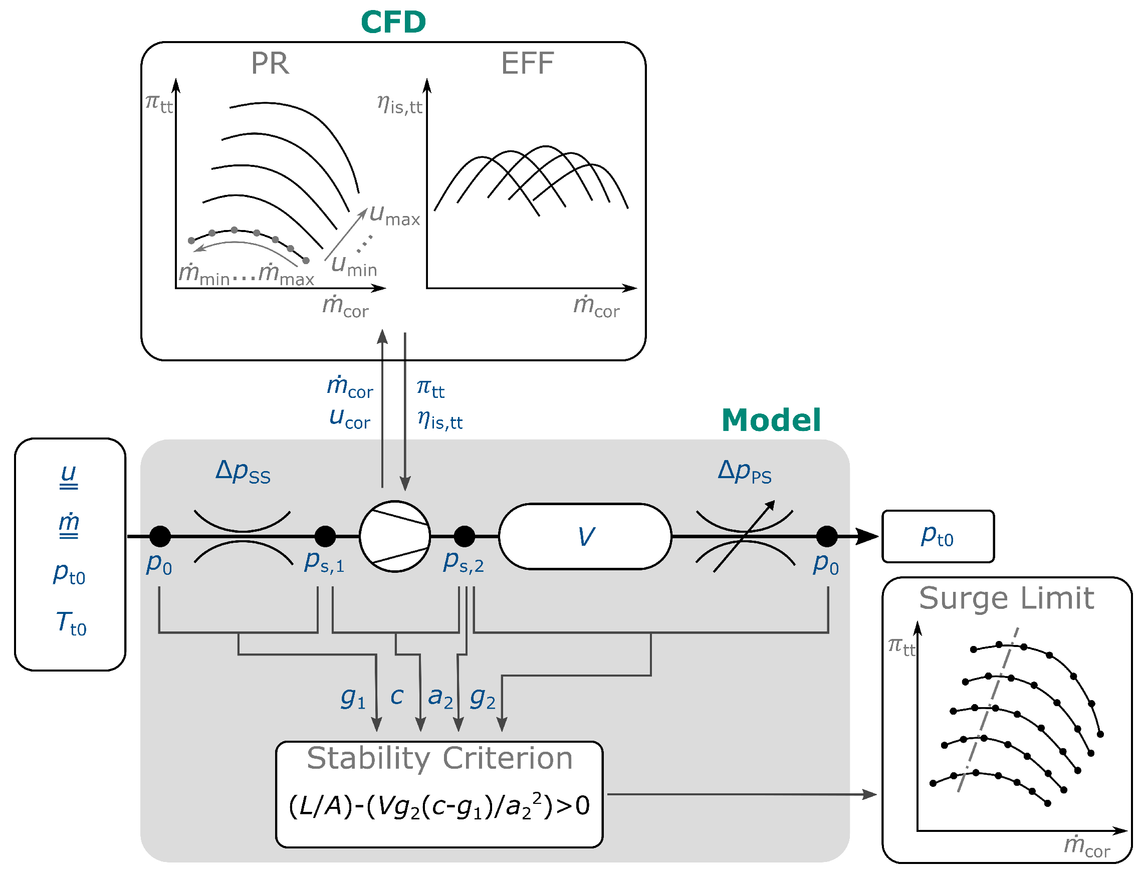
2.1. Methodology—Analytical Modeling of the Compression System

The procedure of the approach should be demonstrated by Figure 2. The core of it is the part highlighted by the gray box. This part basically represents the flow path including the compressor and flow variables like the pressure, temperature and velocity, which are calculated along this flow path. To do so, some information about the system is needed. Starting at the inlet, this is provided by a polynomial for the pressure loss as a function of mass flow rate for the intake section (labeled Inlet throttle in Figure 2). Information about the compressor wheel is provided as pressure ratio ${\mathrm{\Pi }}_{\mathrm{tt}}$ and isentropic efficiency ${\eta }_{\mathrm{is},\mathrm{tt}}$, both versus corrected mass flow rate ${\dot{m}}_{\mathrm{cor}}$. This is the connection of steady-state CFD-simulations and the analytical model, or in other words, the system. The compressor outlet throttle (labeled Outlet throttle in Figure 2) is used to set the operating point of the compressor in the real application. Since the pressure loss across the throttle is dependent on the pressure and flow rate at the throttle inlet, the geometry of the throttle and, thus, the pressure loss versus mass flow rate curve is different for any operating point.

After calculating the static pressure at any section along the flowpath, some further values can be derived. This, in particular, is the throttle characteristic for the inlet system, the compressor characteristic and the throttle characteristic for the outlet system. Characteristic, in this case, stands for the gradient of the static pressure difference over the particular section versus the mass flow rate. All of these values are used in the final stability criterion, Equation (2), to check whether the system is stable or not. Stability, in this case, means that the system surges or not.

$$\begin{array}{cc}\hfill D_{\mathrm{S}}& =\frac{L}{A}-\frac{V·g_2·(c-g_1)}{a_2^2}\hfill \\ \hfill \mathrm{Stable}:D_{\mathrm{S}}& >0\hfill \\ \hfill \mathrm{Unstable}:D_{\mathrm{S}}& <0\hfill \end{array}$$

(2)

For the derivation of Equation (2), the compression system is simplified by a replacement system, as schematically shown in Figure 1b and Figure 2. In accordance with [1], the compressor is represented by an actuator disk placed in a pipe of a representative length and cross-sectional area. Downstream of the compressor stage, the piping is represented by a plenum with a certain volume. The pressure loss upstream of the compressor inlet is modeled as a throttle, comparable to the throttle downstream of the plenum, to set the compressor operating point.

The dynamic behavior of the compression system can then be modeled by formulating two conservation equations. Firstly, for the subsystem from the ambient to the compressor stage outlet, the one-dimensional momentum equation is formulated. Secondly, for the subsystem from the compressor stage outlet to the ambient, the continuity equation for the plenum is formulated. Both equations result in a system of equations, for which the characteristic polynomial can be determined based on the small perturbation analysis. Similarly to structural dynamic theory and analogous to the mass-spring-damper-system, the equation of the damping ratio can be defined. If the value of the damping ratio is less than zero, the system is attenuated and, thus, unstable. In contrast to that, the system is stable if the damping ratio is greater than zero, meaning energy is dissipated during the oscillation process. Taking only the part of the equation of the damping ratio which can be smaller than zero results in the stability criterion $D_{\mathrm{S}}$ in Equation (2). Further details on the derivation can be taken from [19,20].

By evaluating the damping ratio only, nothing can be said about the actual oscillation amplitude. For this reason, it can only be distinguished between a stable and unstable state of the system. Details about the nature of the instability cannot be determined from this. Thus, it cannot be distinguished between deep surge and mild surge by this approach. However, the advantage is that the system of equations does not have to be solved, which makes the procedure much more efficient. Furthermore, in an industrial environment, both types of surge have to be avoided and, therefore, it is mainly of interest if the system surges (unstable) at all or not.

In Equation (2), L and A are defining the length of the inlet piping and the cross-sectional area of the inlet piping, V the volume of the compressor outlet plenum, c the compressor characteristic, $g_1$ the inlet throttle characteristic, $g_2$ the outlet throttle characteristic and $a_2$ the speed of sound in the outlet plenum. Any of the values in Equation (2) are dependent on the current operating point and system. For any operating point in the compressor map, the stability criterion is used to check if the operating point is stable or not. From all of the stable operating points for a certain speedline, the one at the smallest mass flow rate is defining the surge limit.

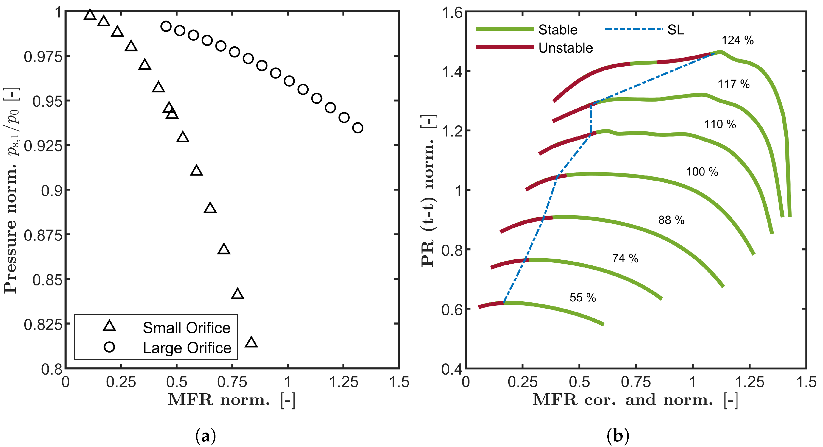
2.2. The Resulting Surge Limit for a System with Inlet Pressure Losses

In this section, the surge limit for a compressor in an application-oriented environment will be determined based on steady-state CFD-simulations. The system represented by the stability model will be called System 1 from now on and is the turbocharger test rig at Tu Darmstadt. The setup and all of the specifications of this test rig have been published by Dielenschneider et al. [21]. The physical (constant) parameters necessary for the stability equation can be taken from

Table 1. Physical parameters for the investigated systems.

Parameter	Calculation	System 1	System 2
L	Environment to compressor inlet	7.5 m	0.25 m
A	Impeller intake cross section	6.21 × 10 −4 m2	6.21 × 10 −4 m2
V	Outlet plenum	1.29 × 10 −3 m3	1.29 × 10 −3 m3

. One additional detail should be pointed out here, again. The mass flow rate is determined by two differently sized orifices far upstream of the compressor inlet. The size of the orifice is chosen to be adequate for a certain mass flow rate range. Furthermore, the mass flow rate measurement system includes some additional components like air filter, piping and flow straightener. All together, these components are creating a pressure loss from ambient to the compressor inlet as a function of the currently selected orifice and the mass flow rate. The pressure characteristic, representing the pressure loss for the mentioned system, is depicted in Figure 3a for both orifice sizes. The pressure is normalized by the ambient pressure. The pressure loss in the case of the small orifice is almost up to 15%.

Passing this information together with all of the other specific system information to the stability model and calculating the system stability for the complete compressor map (determined by steady-state CFD-simulations) results in the surge limit depicted in Figure 3b. This figure is showing the numerically determined compressor speedlines, and the color of the speedlines indicate if the system is stable or not at a particular mass flow rate. The surge limit (blue dashed line) is defined by the last stable operating point, starting at large mass flow rates. A closer look should be taken on the 117% speedline. The surge limit is far away from the peak pressure ratio, well located in a region of positive or zero pressure ratio gradient. This is noteworthy, since a rule of thumb is that a positive pressure ratio gradient is a good indicator for an unstable region in the compressor map. The reason for not becoming unstable is the inlet pressure being a function of the mass flow rate and its influence on the compressor characteristic c. This fact will be further explained in the next section by applying the stability model onto a system without any intake losses. From the 124% speedline, another remarkable fact can be seen. Stable and unstable operating points can apparently alternate. If the surge limit is determined as in the experiment by throttling the compressor at a fixed compressor speed and starting from the choke limit, the surge limit would be at the first unstable area. Crossing this unstable area by quickly throttling the compressor, it might be possible to reach a stable operating point again at a lower mass flow rate for the same compressor speed. This reveals an uncertainty in determining the experimental surge limit. By making a large mass flow rate step when throttling the compressor, it might be possible to jump over unstable areas and determine the surge limit at a lower mass flow rate.

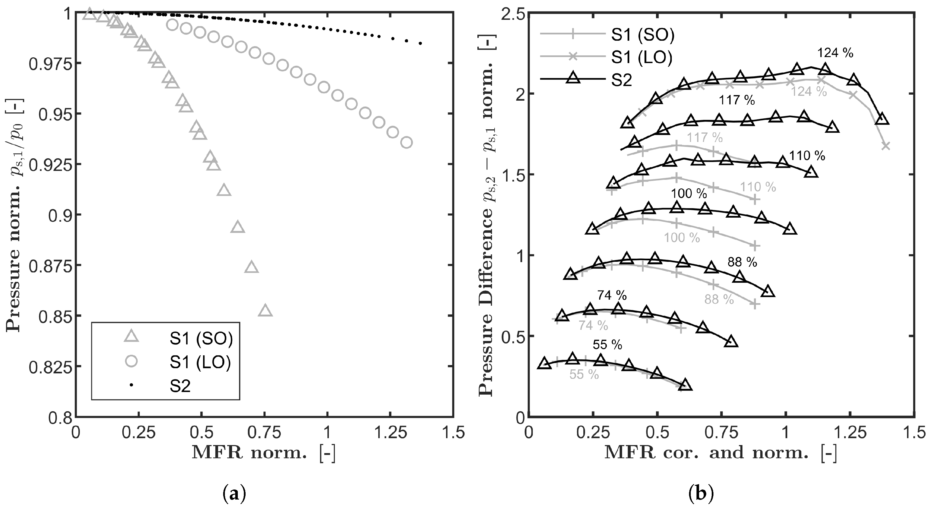
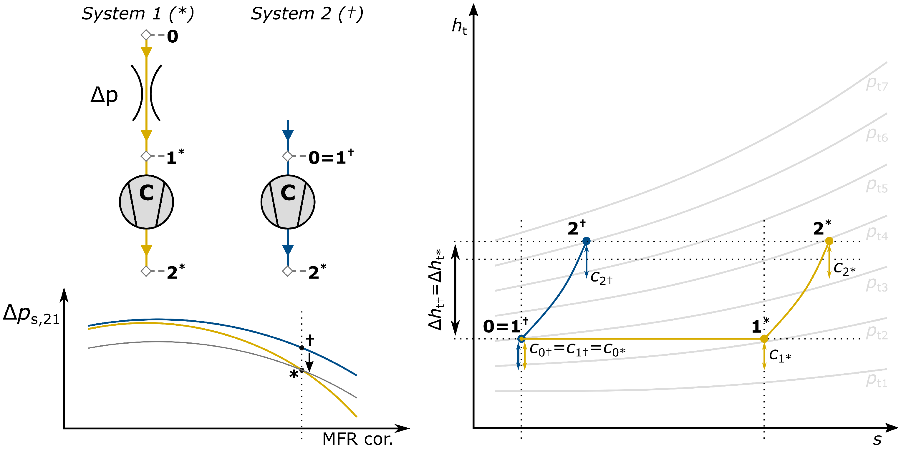
2.3. Variation of the Inlet Pressure Loss and Its Influence on the Surge Limit

A great advantage of the stability model is the possibility to investigate the operation of the compressor stage in different environments. The inlet pressure loss curve is simply replaced by a curve that represents the pressure loss of an air filter only. Since the rest of the system remains unchanged, the compressor map provided to the stability model is still based on the same steady-state CFD-simulations, as in the case of System 1. The current system will be called System 2 from now on. Again, the physical (constant) parameters necessary for the stability equation can be taken from Table 1. The now-specified compressor inlet pressure can be taken from Figure 4a in comparison to the pressure from the preceding section. The intake pressure loss is significantly reduced (black dots, below 2% of ambient pressure), resulting in a much lower gradient of the inlet throttle characteristic. Before analysing the influence of the inlet pressure on the surge limit, the influence on the pressure difference over the compressor $(p_{\mathrm{s},2}-p_{\mathrm{s},1})$ should be analyzed. The slope of this curve is the compressor characteristic c, which is one input parameter of the stability equation. The pressure difference for both systems (System 1 and 2) is depicted in Figure 4b. From this figure, it is remarkable that System 1 and System 2 result in different compressor characteristics even though the same compressor map, determined by steady-state CFD-simulations, has been used. Important to notice is the fact that not only the absolute value has changed but also the sign of the local gradient. And, this is most important for the system stability.

Based on this fact and Figure 4b, the compressor map can be separated into two regions. The first one (Region 1) contains all of the lower speedlines (55% to 100%). In this case, the inlet pressure loss changes the absolute value of the gradient only and not the sign. The change in the sign in the compressor characteristic is almost at the same mass flow rate when comparing System 1 and System 2. The second region (Region 2) applies to speedlines where the pressure ratio curve (${\mathrm{\Pi }}_{\mathrm{tt}}vs.{\dot{m}}_{\mathrm{cor}}$) shows a less pronounced peak, a very flat region or even a local and global maximum. Speedlines 110% to 124% belong to this group. In this case, the inlet pressure loss has a significant influence on the sign of the compressor characteristic c and on the location, where the change in sign is located. The inlet pressure loss apparent in System 1 results in a purely negative gradient until the surge limit. This is favourable for the system stability. Removing or reducing the inlet pressure loss leads to a change in sign at larger mass flow rates. For non-existent inlet pressure losses, the course of the pressure difference $(p_{\mathrm{s},2}-p_{\mathrm{s},1})$ follows the course of the total pressure ratio. This makes the system possibly unstable at larger mass flow rates.

2.3.1. The Compressor Enthalpy Rise

The reason for the different pressure deltas ($\Delta p_{\mathrm{s},21}$) can be explained by the enthalpy–entropy curves of the compression process for different compressor inlet pressures (cf. System 1 and System 2), depicted in Figure 5. The lines are drawn in an idealized form, but this should be sufficient enough to explain the fundamental processes. The following assumptions and simplifications have been made:

• Air as ideal gas;
• The change in kinetic energy across a throttle is negligible;
• The compressor wheel (and no diffuser) is considered only;
• Reynolds number effects are neglected.

The assumption of a constant kinetic energy across the throttle is important, since the influence on the static pressure upstream and downstream of the compressor wheel needs to be assessed. Strictly speaking, only the total enthalpy is constant across a throttle and not the static enthalpy. According to the Fanno-curve, as shown and explained in [22], a constant static enthalpy is only applicable if the pressure difference and, thus, the density change across the throttle is small. In the present case, this condition is considered to be fulfilled in good approximation, since the velocity upstream of the throttle and the pressure loss across the throttle is small.

Both systems are compared for the same operating point, implying the same corrected mass flow rate and circumferential speed. The reference section for the correction is the compressor inlet section, labeled with 1 in the following paragraph. Due to the underlying Mach similarity and the assumptions above, the velocity at the compressor inlet is the same for both systems. Proceeding with that and applying the Euler Turbine Equation in Equation (3), it can be said that the total enthalpy rise across the compressor $\Delta h_{\mathrm{t},\mathrm{C}}$ equals for both systems.

$$\Delta h_{\mathrm{t},\mathrm{C}}=0.5·(v_2^2-v_1^2+w_1^2-w_2^2+u_2^2-u_1^2)$$

(3)

Saying that the total enthalpy rise $\Delta h_{\mathrm{t}}$ and the entropy production $\Delta s$ of the compression process ($1\to 2$) equals for both systems and that an isobar can be expressed by an exponential expression ($h_{\mathrm{t}}=h_{\mathrm{ref}}·e^{s/c_{\mathrm{p}}}$) leads to the equation of the total enthalpy ratio, Equation (4). In this equation, $h_{\mathrm{ref}}$ is defining the enthalpy of an isobar at a reference state and thus setting the pressure level of this certain isobar. Reformulating the initial fraction results in the fact that the total pressure ratio ${\mathrm{\Pi }}_{\mathrm{tt},\mathrm{C}}$ is the same for both systems.

$$\frac{h_{{\mathrm{t}2}^{†}}}{h_{{\mathrm{t}1}^{†}}}=\frac{h_{{\mathrm{ref},2}^{†}}}{h_{{\mathrm{ref},1}^{†}}}·\cancel{e^{\frac{\Delta s_{{}^{†}}}{c_{\mathrm{p}}}}}=\frac{h_{{\mathrm{ref},2}^{*}}}{h_{{\mathrm{ref},1}^{*}}}·\cancel{e^{\frac{\Delta s_{{}^{*}}}{c_{\mathrm{p}}}}}\to \frac{p_{{\mathrm{t},2}^{†}}}{p_{{\mathrm{t},1}^{†}}}=\frac{p_{{\mathrm{t},2}^{*}}}{p_{{\mathrm{t},1}^{*}}}$$

(4)

With all of the facts above, the cycles from the ambient, through the inlet section and the compressor wheel, can be outlined in the h-s-diagram for both systems, in the case of the total enthalpy at first. Again, both cycles are drawn for the same operating point of the compressor in case of corrected mass flow rate and circumferential speed. The difference is, mainly, the compressor inlet pressure, due to the modified inlet section. Position 0 is representing the ambient boundary condition. Position 1 and Position 2 are the conditions upstream and downstream of the compressor wheel. In case of System 2, states 0 and $1^{†}$ are the same. The compressor sucks in air from the environment. The corresponding line in the h-s-diagram is the blue line.

In case of System 1, there is a throttle between the ambient and the compressor inlet. The total enthalpy across this throttle ($0\to 1^{*}$) is constant. The compressor inlet pressure (total, $1^{*}$) is, thus, lower than the ambient pressure. From state $1^{*}$ to state $2^{*}$, the same total enthalpy rise as for System 2 is applied to the fluid. The major difference comes from the exponential course and the resulting divergence of the isobars. The divergence increases for larger entropies. It is not important at what exact values the process is running. It is just important to see that the compression process for System 1 runs in a region with an increased divergence of the isobars compared to System 2. This is the reason why a lower total pressure difference from state $1^{*}$ to state $2^{*}$ is achieved.

What matters more for the system stability, however, is the static pressure difference. Based on the assumptions above and the fact that the velocity at any position along the flowpath for both systems equal, the cycles in the h-s-diagram are comparable in case of the static enthalpy. For this reason, the same as for the total pressure difference applies to the static pressure difference. The influence on the system stability should now be demonstrated by the diagram at the lower left corner of Figure 5. If the pressure at the inlet would be decreased constantly for all operating points along a speedline (e.g., operation at higher altitude), the pressure difference $\Delta p_{\mathrm{s},21}$ would be lowered constantly (blue line → grey line). There would be no influence on the compressor characteristic (i.e., gradient is unaffected). If the pressure at the inlet is not lowered constantly but as a function of the mass flow rate, the gradient of the pressure difference $\Delta p_{\mathrm{s},21}$ and, thus, the compressor characteristic is altered (blue line → yellow line).

2.3.2. The Stability Map

Now, determining the stability for all operating points of the compressor map results in the stability map, depicted in Figure 6a. This figure is comparable to Figure 3b. The difference is in the color, which is now indicating the stability for System 2. For the speedlines belonging to Region 1, nothing surprising happens. All operating points on the right side of the surge limit are stable and the remaining ones the left side of the surge limit are unstable. For speedlines belonging to Region 2, the surge limit is now shifted to larger mass flow rates. Following the procedure as in the experiment and taking the last stable operating point as the surge limit results in the surge limit depicted in Figure 6b. The blue solid line is showing the surge limit for System 2 in comparison to the surge limit for System 1 (yellow line). This shows that the influence of the inlet pressure can be significant, depending on the shape of the speedline.

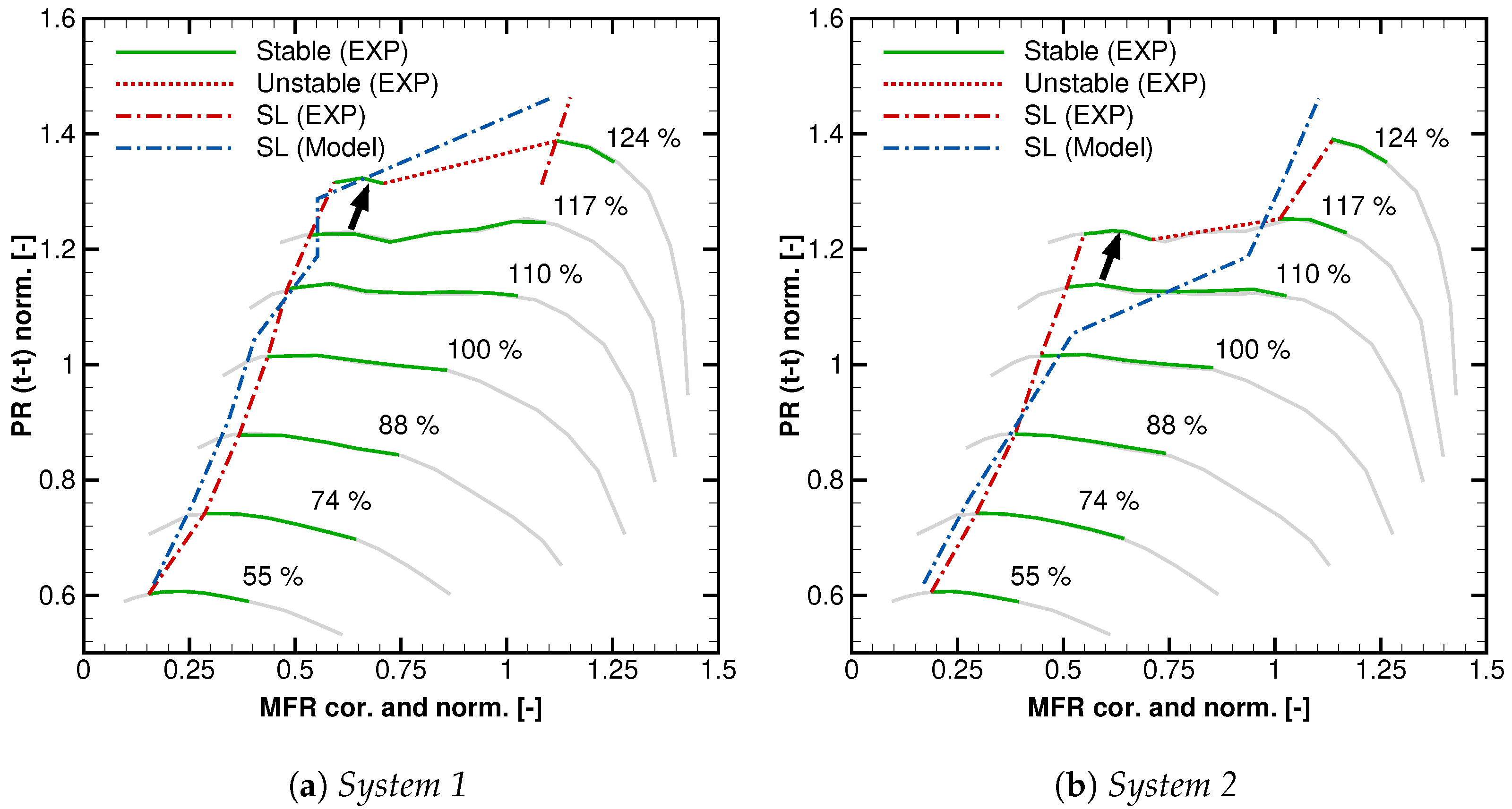
3. Experimental Validation

The results of the experimental investigation are depicted in Figure 7 for System 1 (Figure 7a) and System 2 (Figure 7b). The grey solid lines are showing a reference compressor map, which has been gained experimentally through a maximum reduction in the outlet plenum volume. The reference map is the same in Figure 7a,b. The green solid lines are showing operating points that have been measured for System 1 and System 2 and the color is indicating that these operating points are stable. By comparing the green with the grey lines in both cases, it can be confirmed that the total pressure ratio is unaffected by the compressor inlet pressure.

For the validation of the surge limit for System 1, two different regions in the compressor map need to be distinguished. In case of the 55% to 117% speedlines, there is only one surge limit. In case of the 124% speedline, two surge limits can be determined experimentally. Coming from the choke limit, the first surge limit will be reached. Beyond this limit (red dashed line, unstable), the compressor can not be operated safely. Referring to Figure 3b, there should be another stable area at lower mass flow rates according to the stability model. By accurately sticking to the speedline, this area is not reachable. But, as shown by the experimental data, this area can be reached by approaching it from a lower speedline, like shown by the black arrow in Figure 7a. Through this procedure, a second surge limit can be determined.

At this point, the following three facts can already be concluded from the experimental investigation:

• There can be multiple surge limits for one speedline;
• The experimental and numerical surge limits match very well;
• The alternating stable and unstable regions can be predicted very well.

The influence of the compressor inlet pressure can now be analyzed by Figure 7b. The compressor map can again be divided into different regions. There is the first region at lower compressor speeds, including the speedlines 55% to 100%. For this region, there is only one surge limit, which is not significantly affected by the inlet pressure. The next region consists of the speedlines 110% and 117%. Referring to Figure 6a, the stability model predicts alternating stable and unstable areas. In case of the 110% speedline, the experimental data is showing only one surge limit and at much lower mass flow rates than the stability model based on the steady-state CFD-simulations. The predicted unstable areas are either predicted wrong or too small to be captured by the experiment. In the case of the 117% speedline, the unstable area is predicted much larger and now the experimental data is showing two surge limits. There is one at a larger mass flow rate and one at a lower mass flow rate. The second surge limit and the operating points close to it can again be determined by the procedure mentioned for System 1. This is shown by the black arrow in Figure 7b. The last speedline, 124%, belongs to the third region. This region shows only one surge limit, comparable to the first region. Finally it can be concluded that the experimental and numerical surge limit match very well, except for one speedline.

4. Conclusions

The goal of the paper was to present a methodology on how to determine a surge limit by means of numerical simulations and a Greitzer surge model. To do so, the connection between different system parameters and the system stability must be understood and considered. For this reason, mainly two different systems have been investigated experimentally and analytically. Since the influence of the compressor outlet system is already understood very well, the focus of the system variation within this investigation had been on the compressor inlet system. Based on these variations, the following concluding remarks can be drawn.

4.1. The System Influence on Stability Limiting Parameters

A rule of thumb is that a negative speedline gradient is superior for the system stability. Since the gradient of the static pressure difference over the compressor stage is relevant for the system stability and not the gradient of the total pressure ratio, this is only valid for a constant compressor inlet pressure. If the compressor inlet pressure is a function of the mass flow rate, there is an interaction with the compressor wheel that can lead to a negative gradient of the pressure difference even if the speedline gradient is positive.

4.2. The Numerical Convergence Is No Good Indicator for Surge

If the simulation domain consists of the compressor stage only, like is often the case to save numerical resources, the system influence is not considered. The numerical stability, or in other words the numerical convergence, is, thus, a matter of the numerical setup and not of the system stability.

4.3. There Is Not a Single Surge Limit

Surge is a phenomenon that is influenced by multiple system parameters and not only dependent on the compressor wheel or stage. Since most of the influencing parameters are functions of the mass flow rate, stable and unstable areas in the compressor map can exist alternately. An important requirement for this to happen is either a flat speedline or a speedline with a local and global maximum. In this case, the surrounding system parameters and their interaction with the compressor stage can stabilize the system.

4.4. Modeling the System Dynamic Behavior Is Necessary to Determine a Surge Limit

The system dynamic behaviour needs to be considered in any way when determining the surge limit by means of numerical simulation data. A practicable method has been shown within this paper by using an analytical surge model based on the Greitzer approach. The usage of commercial 1D gas dynamic tools could also be a feasible way.

References

1. Greitzer, E.M. Surge and Rotating Stall in Axial Flow Compressors—Part I: Theoretical Compression System Model. J. Eng. Power 1976, 98, 190–198. [Google Scholar] [CrossRef]
2. Greitzer, E.M. Surge and Rotating Stall in Axial Flow Compressors—Part II: Experimental Results and Comparison with Theory. J. Eng. Power 1976, 98, 199–211. [Google Scholar] [CrossRef]
3. Fink, D.A.; Cumpsty, N.A.; Greitzer, E.M. Surge Dynamics in a Free-Spool Centrifugal Compressor System. J. Turbomach. 1992, 114, 321–332. [Google Scholar] [CrossRef]
4. Grapow, F.; Liśkiewicz, G. Study of the Greitzer Model for Centrifugal Compressors: Variable Lc Parameter and Two Types of Surge. Energies 2020, 13, 6072. [Google Scholar] [CrossRef]
5. Powers, K.H.; Brace, C.J.; Budd, C.J.; Copeland, C.D.; Milewski, P.A. Modeling Axisymmetric Centrifugal Compressor Characteristics From First Principles. J. Turbomach. 2020, 142, 091010. [Google Scholar] [CrossRef]
6. Powers, K.H.; Kennedy, I.J.; Brace, C.J.; Milewski, P.A.; Copeland, C.D. Development and Validation of a Model for Centrifugal Compressors in Reversed Flow Regimes. In Volume 8: Industrial and Cogeneration, Manufacturing Materials and Metallurgy, Marine, Microturbines, Turbochargers, and Small Turbomachines; American Society of Mechanical Engineers: New York, NY, USA, 2020. [Google Scholar] [CrossRef]
7. Powers, K. Development and Validation of a Mathematical Model for Surge in Radial Compressors. Ph.D. Thesis, University of Bath, Bath, UK, 2021. [Google Scholar]
8. Powers, K.H.; Kennedy, I.J.; Brace, C.J.; Milewski, P.A.; Copeland, C.D. Development and Validation of a Model for Centrifugal Compressors in Reversed Flow Regimes. J. Turbomach. 2021, 143, 101001. [Google Scholar] [CrossRef]
9. Powers, K.; Kennedy, I.; Archer, J.; Eynon, P.; Horsley, J.; Brace, C.; Copeland, C.; Milewski, P. A New First-Principles Model to Predict Mild and Deep Surge for a Centrifugal Compressor. Energy 2022, 244, 123050. [Google Scholar] [CrossRef]
10. Yoon, S.Y.; Lin, Z.; Goyne, C.; Allaire, P.E. An Enhanced Greitzer Compressor Model Including Pipeline Dynamics and Surge. J. Vib. Acoust. 2011, 133, 051005. [Google Scholar] [CrossRef]
11. Dielenschneider, T.; Ratz, J.; Leichtfuß, S.; Schiffer, H.P.; Eißler, W. On the Challenge of Determining the Surge Limit of Turbocharger Compressors: Part 1 - Experimental and Numerical Analysis of the Operating Limits. In Volume 6: Ceramics and Ceramic Composites, Coal, Biomass, Hydrogen, and Alternative Fuels, Microturbines, Turbochargers, and Small Turbomachines; American Society of Mechanical Engineers: New York, NY, USA, 2021. [Google Scholar] [CrossRef]
12. Semlitsch, B.; Jyothishkumar, V.; Mihaescu, M.; Fuchs, L.; Gutmark, E.J. Investigation of the Surge Phenomena in a Centrifugal Compressor Using Large Eddy Simulation. In Volume 7A: Fluids Engineering Systems and Technologies; American Society of Mechanical Engineers: New York, NY, USA, 2013. [Google Scholar] [CrossRef]
13. Semlitsch, B.; Mihăescu, M. Flow Phenomena Leading to Surge in a Centrifugal Compressor. Energy 2016, 103, 572–587. [Google Scholar] [CrossRef]
14. Sundström, E.; Semlitsch, B.; Mihăescu, M. Generation Mechanisms of Rotating Stall and Surge in Centrifugal Compressors. Flow Turbul. Combust. 2017, 100, 705–719. [Google Scholar] [CrossRef] [PubMed]
15. Margot, X.; Gil, A.; Tiseira, A.; Lang, R. Combination of CFD and Experimental Techniques to Investigate the Flow in Centrifugal Compressors Near the Surge Line. In SAE Technical Paper Series; SAE International: Warrendale, PA, USA, 2008. [Google Scholar] [CrossRef]
16. Karim, A.; Wade, R.; Morelli, A.; Miazgowicz, K.; Lizotte, B. Surge Prediction in a Single Sequential Turbocharger (SST) Compressor Using Computational Fluid Dynamics. In SAE Technical Paper Series; SAE International: Warrendale, PA, USA, 2019. [Google Scholar] [CrossRef]
17. Dehner, R.; Selamet, A.; Keller, P.; Becker, M. Simulation of Deep Surge in a Turbocharger Compression System. J. Turbomach. 2016, 138, 111002. [Google Scholar] [CrossRef]
18. Haeckel, T.; Paul, D.; Leichtfuß, S.; Schiffer, H.P.; Eißler, W. Determination of a Numerical Surge Limit by Means of an Enhanced Greitzer Compressor Model. In Proceedings of the 15th European Conference on Turbomachinery Fluid Dynamics and Thermodynamics, Paper n. ETC2023-225, Budapest, Hungary, 24–28 April 2023; European Turbomachinery Society: Florence, Italy, 2023. Available online: https://www.euroturbo.eu/publications/conference-proceedings-repository/ (accessed on 13 November 2023).
19. Bühler, J.; Leichtfuß, S.; Schiffer, H.P.; Lischer, T.; Raabe, S. Surge Limit Prediction for Automotive Air-Charged Systems. Int. J. Turbomach. Propuls. Power 2019, 4, 34. [Google Scholar] [CrossRef]
20. Bühler, J. Über den Einfluss Aerodynamischer Effekte und Systemischer Größen auf das Kennfeld von Radialverdichtern. Ph.D. Thesis, Shaker Verlag, Düren, Germany, 2020. [Google Scholar] [CrossRef]
21. Dielenschneider, T.; Bühler, J.; Leichtfuß, S.; Schiffer, H.P. Some Guidelines for the Experimental Characterization of Turbocharger Compressors. In Proceedings of the European Conference on Turbomachinery Fluid Dynamics and Thermodynamics, Lausanne, Switzerland, 8–12 April 2019; European Turbomachinery Society: Florence, Italy, 2019. [Google Scholar] [CrossRef]
22. Baehr, H.D.; Kabelac, S. Thermodynamik; Springer: Berlin/Heidelberg, Germany, 2016. [Google Scholar] [CrossRef]
Figure 1. Simplified schematic of a turbocharged ICE (a), test rig (b) and CFD (c).
Ijtpp 08 00048 g001
Figure 2. Definition of system parameters along the flowpath influencing the surge limit determination and their interaction.
Ijtpp 08 00048 g002
Figure 3. Compressor inlet pressure p s , 1 (a) and the surge limit (b) for System 1.
Ijtpp 08 00048 g003
Figure 4. Compressor inlet pressure p s , 1 (a) and the influence on the static pressure difference p s , 2 p s , 1 (b); Comparison of System 1 and System 2.
Ijtpp 08 00048 g004
Figure 5. The compression system in the h-s-diagram.
Ijtpp 08 00048 g005
Figure 6. The system stability throughout the compressor map and the surge limit for System 2 (a) and the surge limits for System 1 and System 2 in comparison (b).
Ijtpp 08 00048 g006
Figure 7. Comparison of the experimental and numerical surge limit.
Ijtpp 08 00048 g007