Abstract
This paper derives and validates an analytical model for acoustic boundary conditions on a can-annular gas turbine combustion system composed of discrete cans connected to an open annulus upstream of a turbine. The analytical model takes one empirical parameter: a connection impedance between adjacent cans. This impedance is extracted from time-marching computations of two-can sectors of representative combustors. The computations show that reactance follows the Rayleigh conductivity, while resistance takes a value of order 0.1 as a weak function of geometry. With a calibrated value of acoustic resistance, the analytical model reproduces can-to-can transfer functions predicted by full-annulus computations to within 0.03 magnitude at compact frequencies. Varying the combustor–turbine gap length, both model and computations exhibit a minimum in reflected energy, which drops by 63% compared to the datum gap. A parametric study yields a design guideline for gap length at the minimum reflected energy, allowing the designer to maximise transmission from the combustion system and reduce damping requirements.
1. Introduction
In gas turbine combustors, thermoacoustic instability is a self-excited oscillation caused by feedback between unsteady heat release and acoustic waves. The resulting large pressure fluctuations are undesirable for noise and structural design considerations. In-phase pressure and heat release perturbations act as a source of acoustic energy, which a designer balances against acoustic losses by transmission through the turbine and damping devices. Therefore, predicting thermoacoustic instability requires a combustor model with accurate boundary conditions to characterise waves reflected from the turbine interface.
Industrial gas turbines use can-annular combustion systems, where transition ducts connect discrete burners to an axial gap upstream of the turbine nozzle guide vane. Due to rotational symmetry, historical design practice has assumed a single can to be a good model of the entire combustion system. This simplification is convenient, as experimental or computational costs scale with the number of cans under test, but neglects coupling between adjacent cans by azimuthal waves.
Kaufmann et al. [1] measured a peak in the pressure fluctuation spectra of an annular rig which was not present in a single-can test. Quarter-annulus thermoacoustic computations were sufficient to capture the extra peak, and revealed that it corresponds to a ‘push-pull’ mode where adjacent cans oscillate in antiphase. Venkatesan et al. [2] showed experimentally that blocking the connection area in the combustor–turbine gap suppressed a ‘push–pull’ mode in their two-can test apparatus.
Ghirardo et al. [3] performed Helmholtz simulations of a can-annular combustor and provided experimental evidence of their predicted azimuthal mode shapes. The simulations yielded boundary conditions suitable for thermoacoustic modelling: acoustic wave transfer functions between all possible can pairs. They emphasise that stability is a system property and can only be determined by a system thermoacoustic model including a ring of reacting burners linked by a complete set of can-to-can transfer functions.
In an iterative design process, a low-order model is useful to complement more time-consuming experimental testing or numerical computations. von Saldern et al. [4] used mass conservation over a compact gap and a Rayleigh conductivity for the connection impedance between adjacent cans to develop analytical expressions for can transfer functions at low reduced frequencies. Their predictions are qualitatively similar to the can transfer functions from the simulations of Ghirardo et al. [3]. Fournier et al. [5] showed that augmenting the Rayleigh conductivity with a characteristic length, a function of azimuthal mode empirically fitted from two-dimensional Helmholtz simulations, matches acoustic impedance phase results to within 2%.
Overall, the literature shows that a single-can combustor model, lacking communication between cans, is not representative of a can-annular combustor. The connection impedance model of von Saldern et al. [4] is promising; instability frequencies in large industrial gas turbines are typically low and in the compact regime. However, the empirical connection impedance parameter has not been characterised in fully representative configurations.
The present work first determines the sensitivity of connection impedance to geometry by extracting values from non-linear time marching computations of two-can combustor sectors. Then, analytical and numerical full-annulus predictions of can transfer functions are compared. Finally, the analytical model is used to explore the can-annular combustor design space.
This paper, an extended version of a previous conference submission [6], makes the following contributions:
- Validation of the von Saldern et al. [4] connection impedance model in an industrially representative can-annular combustor;
- Clarification of the importance of intra-can acoustic resistance in predicting can-to-can transfer functions;
- A new design guideline for selection of combustor–turbine gap to minimise reflected energy, hence easing stability issues by reducing the required damping.
2. Connection Impedance Analytical Model
The current analytical model follows the method proposed by von Saldern et al. [4] and later extended by Orchini [7]. This section gives a derivation that includes the effect of a general downstream impedance without other complications. In outline: the model conserves mass over the combustor–turbine gap, an empirical connection impedance relates intra-can velocities with pressure fluctuations in adjacent cans, and a Fourier series relates the pressure in adjacent cans by a phase shift.
The model makes four assumptions: (i) acoustic wavelength is much larger than can or gap cross-sections, so that the gap is compact; (ii) the combustor comprises N identical cans each with symmetry about a constant- plane; (iii) there is no mean flow in the gap; (iv) the combustor connects to a turbine with known (non-dimensional) acoustic impedance to plane pressure waves, .
Although further analytical models are available for , in this paper, the downstream turbine impedance is prescribed using CFD results for plane wave forcing in an open annulus after Brind and Pullan [8], isolating errors in the combustor model from possible errors in a turbine analytical model.
Figure 1 shows notation required for the derivation. The real three-dimensional combustor and turbine geometry in Figure 1a, is modelled as the network shown in Figure 1b. Each of the combustor cans has a control volume, CVn, defined over its sector of the combustor–turbine gap. The analytical model provides an acoustic impedance at the leading edge of CVn to be used as a boundary condition in a separate thermoacoustic calculation of the combustor cans.
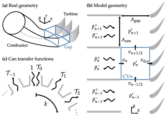
Figure 1.
Notation for connection impedance analytical model: (a) real combustor and turbine geometry, with control volume; (b) model geometry with quantities required for the derivation; (c) definition of can transfer functions . Note that cans may be oriented axially or radially.
In the compact regime, the acoustic pressure perturbation is uniform over each control volume, and the velocity perturbations v are uniform over each of the four bounding control surfaces. Within the assumptions of the model, can transfer functions are independent of the detailed shape of the combustor, and two areas and are sufficient to characterise the geometry. This means that the cans may be oriented axially or radially.
With quantities defined in Figure 1b, conservation of mass in control volume CVn requires
To evaluate intra-can velocities, define a non-dimensional impedance of the connections between cans,
and substitute into Equation (1),
Invoking linearity, a general circumferential distribution of pressure fluctuations can be expressed as a Fourier series,
where a tilde denotes amplitudes of the azimuthal harmonics. At fixed azimuthal mode m, pressures in two adjacent cans spaced an angle apart are related by a phase shift . Substituting the phase shift into Equation (3) and simplifying using trigonometric identities,
Then, rearranging for the overall impedance at a given azimuthal mode,
When building a thermoacoustic model, it is more convenient to work with can transfer functions , as shown in Figure 1c, instead of modal impedances . The kth transfer function is defined to reflected waves in an arbitrary can, from incident waves in another can offset k positions away,
where a hat denotes characteristic wave amplitudes,
Following Ghirardo et al. [3], the can transfer functions are given by the inverse discrete Fourier transform of modal reflection coefficients ,
Equation (9) is justified as follows. Forcing a single can is equivalent to an impulse in the can domain and so excites all azimuthal modes equally. The acoustic response in the modal domain is weighted by the reflection coefficients at each harmonic. Taking the inverse Fourier transform returns to the can domain and yields the reflected waves in each can resulting from the original impulse.
3. Time-Marching Computational Approach
This section describes the computational fluid dynamics approach of the present work, following methods developed by Brind and Pullan [8]. Applying forcing to non-linear time-marching computations and analysing the resulting acoustic response allows can transfer functions to be calculated.
3.1. Domain and Boundary Conditions
The datum combustor and turbine under consideration are representative of a large industrial gas turbine. The combustor comprises cylindrical cans, each identical and symmetric about a constant- plane, connecting via transition ducts to an open annulus upstream of the turbine. The analytical model does not describe acoustic behaviour upstream of the can trailing edge, so a simplified can geometry omitting fuel injectors and cooling flows is sufficient for these validation calculations. An axial gap of length separates combustor and turbine. Figure 2 illustrates schematically the computational domain and boundary conditions.
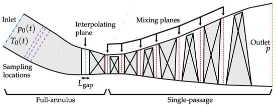
Figure 2.
Domain and boundary conditions for coupled combustor and turbine CFD simulations.
The turbine design is a realistic four-stage geometry with coolant flows, leakage flows, and three-dimensional blading. Surface patches, imposing additional fluxes of mass, momentum, and energy, inject a total coolant flow of order 25% the turbine inlet mass flow. Flow is subsonic, with a Mach number of in the combustor and a vane exit Mach number of . The Reynolds number, based on nozzle guide vane axial chord and exit velocity, is of order .
To capture all possible azimuthal modes, the computational model couples combustor and nozzle guide vane in a full-annulus configuration, joined to single-passage representations of downstream blade rows using mixing planes. Alternatively, with even N, two-can computational models provide data sufficient to extract a value for connection impedance at reduced computational cost ( is independent of m).
The domain is circumferentially periodic. Inlet boundary conditions are prescribed uniform values of stagnation pressure and temperature; the outlet boundary condition is a prescribed static pressure, with spanwise variations assuming radial equilibrium (Figure 2). Although spatially uniform, the inlet boundary conditions are functions of time. Because the multi-stage turbine allows negligible upstream transmission, reflections from the outlet boundary have no influence on the solution in the combustor. Reflections from the inlet boundaries are accounted for and corrected in post-processing.
A circumferential interpolating plane joins the combustor and nozzle guide vane grids at an interface within the combustor–turbine gap (Figure 2). Interpolation uncouples the pitchwise grid densities of combustor and turbine. Mixing planes connect subsequent rows of the turbine; this model yields a reduction in computational cost of one order of magnitude with negligible loss of accuracy compared to an entirely full-annulus turbine. To confirm this fact, computations with the first three turbine rows full-annulus yielded can transfer functions within 2% of the nozzle guide vane only model.
3.2. Computational Details
Simulations were performed using Turbostream 3, a multi-block structured, compressible, unsteady Reynolds-averaged Navier–Stokes solver developed by Brandvik and Pullan [9]. The code uses a finite-volume formulation that is second-order accurate in space and implicit dual time stepping with a second-order accurate backward difference scheme. The simulations employ an algebraic mixing-length turbulence model: a computationally inexpensive choice that gives accurate results when calibrated against measurements. Nevertheless, the focus of the simulations is inviscid wave propagation, because acoustic viscous effects are confined to a thin boundary layer with thickness of order . The turbulence model only needs to set up a representative mean flow, and quantitative predictions of turbine performance are not essential. A fully-turbulent wall function yields shear stress on solid boundaries, at a distance in wall units. Resolution studies confirmed discretisation independence with at least 100 grid points per acoustic wavelength and 72 time steps per acoustic period. This requires of order nodes in each combustor can and blade passage. Duplicating combustor and nozzle to form a full-annulus sector yields a mesh with 58 × 106 nodes.
In forced computations, inlet boundary conditions take the form
In Equation (10), is a small amplitude parameter, and values of and J are selected to span a reduced frequency range range , where . This frequency range is typical of combustion instability in large industrial machines.
In full-annulus computations, to excite all azimuthal modes, an arbitrary set of can indices are forced, while in the other cans. Preliminary simulations showed that calculated transfer functions were independent of the forcing pattern, confirming that the problem is linear. In two-can computations, both cans are forced in antiphase, exciting the mode only.
Unsteady computations are started from a converged steady solution and run for eight forcing periods, then flow field data are sampled for a further eight forcing periods. One case requires two days of wall-clock time on four Nvidia A100 graphical processing units.
3.3. Post-Processing for Can Transfer Functions
This section describes calculation of can transfer functions from the CFD results to compare with the analytical model. The solver outputs unsteady flow field data at three cross-section sampling planes, shown in Figure 2, for each of the N combustor cans. At each instant in time, the pressure fluctuations are area averaged over the sampling planes to give scalar but unsteady quantities.
The least-squares multi-microphone wave separation technique of Poinsot et al. [10] yields upstream- and downstream-running characteristic wave amplitudes in all N cans, and , from pressure fluctuations on the three sampling planes in each can, given spacings between the planes and the acoustic speed. Phase shifting waves to the centre of the combustor–turbine gap ensures consistency with the analytical model. The segmentation approach of Miles [11,12] accounts for area variation along the transition duct.
Forcing the th can alone, from Equation (9) the reflected wave in the nth can is . In general, the total reflected wave is a linear superposition of contributions from all cans. Summing over k,
Equation (11) is by definition a discrete convolution, of a periodic vector of N transfer functions with a periodic vector of N incident waves to make a periodic vector of N reflected waves . By the convolution theorem, the solution of Equation (11) is where denotes the discrete Fourier transform operator. The formulation of Equation (11) does not require an assumption of non-reflecting inlet boundaries.
3.4. Extracting Connection Impedance
There are two ways to post-process connection impedance, , from a CFD solution. The direct method is to evaluate Equation (2) using area-averaged Fourier-transformed quantities: static pressure on a plane at the can trailing edge and azimuthal acoustic velocity on a plane spanning the gap. The indirect method employs ‘push–pull’ forcing at fixed azimuthal mode . Wave separation on sampling planes away from the can trailing edge, where the acoustics are one-dimensional, yields characteristic wave amplitudes and a reflection coefficient for this mode. Converting to an impedance as in Equation (9), setting , and rearranging Equation (6),
The direct method involves an arbitrary averaging procedure that is not strictly consistent with the assumption of one-dimensional acoustics but applies at all frequencies. The indirect method has no area-averaging but assumes validity of the analytical model and hence only applies at compact frequencies. This paper quotes reactances calculated using the direct method to capture frequency trends and resistances using the indirect method for most consistency with the analytical model.
4. Quantifying Connection Acoustic Impedances
The analytical model takes one empirical parameter: a connection impedance between adjacent cans, defined in Equation (2). This section uses time-marching simulations of two-can computational models to extract values for resistive (lossy) and reactive (inertial) parts of and determine its sensitivity to geometry. Figure 3 shows four geometries used for this study. The ‘Datum’ case is fully representative. The ‘Clocked’ geometry is the datum rotated by half a vane pitch to align combustor can walls with nozzle mid-passage. The ‘Slip’ and ‘Thick’ geometries have square combustor cans of constant cross section, with a zero-thickness inviscid wall and a wall of width 0.36 .
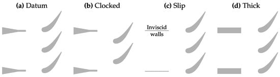
Figure 3.
Four geometries of combustor can: (a) datum can and transition duct, (b) datum clocked by half a vane pitch, (c) square with thin inviscid walls, (d) square with thick trailing edge. Not to scale.
4.1. Acoustic Reactance
Figure 4a shows acoustic reactances, , for the four combustor geometries as a function of reduced frequency . For Datum and Slip cases, is proportional to frequency, as expected for an inertial effect, and within 6% of the classical Rayleigh conductivity . The Clocked reactance has a slope of twice the Rayleigh conductivity. When the combustor wall is not circumferentially aligned with vane leading edges, the volume of fluid in motion and hence inertia is greater than an ideal thin-walled aperture for which the Rayleigh conductivity is derived.
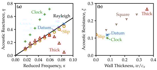
Figure 4.
Connection impedance for different combustor geometries: (a) real part, acoustic reactance; (b) imaginary part, acoustic resistance at . For representative cases, reactance is within 6% of the classical Rayleigh conductivity. Resistance increases linearly with combustor wall thickness.
The Thick combustor has similar reactance to the Datum and Slip cases for . At high reduced frequencies, the Thick reactance departs from a linear trend as the trailing-edge vortex shedding locks in to the forcing frequency. The vortex shedding amplifies acoustic motion and acts to reduce effective inertia. In real combustors, with representative thin trailing edges , the vortex shedding effect is negligible at typical combustion instability frequencies .
4.2. Acoustic Resistance
Figure 4b shows acoustic resistances for the four cases in Figure 3, plus additional square combustors with varying wall thickness. The resistances are calculated using the indirect method at a reduced frequency of and plotted as a function of wall thickness.
All resistances with wall thicknesses fall in the range , a variation of about the mean. The non-zero resistance of the Slip case shows acoustic loss does not require a viscous wake behind the combustor wall, suggesting an inviscid effect is responsible. For the family of Square combustor geometries ranging from , resistance increases linearly from to . A linear increase in resistance is consistent with an effect that scales with connection volume. For the same wall thickness, the Datum and Clocked geometries have smaller values of acoustic resistance compared to the Square combustors, showing that the effect of combustor trailing edge shape, and clocking with the turbine, cannot be neglected.
4.3. Effect of Combustor–Turbine Gap Length
The length of the combustor–turbine gap is a degree of freedom available to the designer, selected by compromise between overall machine size and non-uniformity of the turbine inlet flow field. If the connection impedance were a strong function of gap length, the analytical model would require multiple calibrations to investigate the influence of gap length on can transfer functions.
Translating the Datum combustor in the axial direction, and extracting acoustic resistances for each length from two-can computations, yields the points shown in Figure 5. Over the range acoustic resistance varies by with respect to the representative value . The insensitivity of acoustic resistance over this wide range suggests that the present model can achieve good accuracy with calibration at only a single gap length.
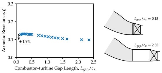
Figure 5.
Acoustic resistance of the Datum combustor with varied axial combustor–turbine gap. Resistance is insensitive to gap length, varying by ±15% over the entire simulated range.
4.4. Physical Mechanism
To identify the physical mechanism for acoustic resistance requires tracking acoustic energy on a local level. Morfey [13] defined a generalised acoustic energy flux,
where and are static pressure and velocity component fluctuations, while , , and a are the mean density, velocity components, and acoustic speed. The first term in Equation (13) is the classical acoustic energy flux after Kirchoff, which is only conserved in a stationary uniform medium; the remaining terms account for a moving medium. Time averaging Equation (13) gives the generalised acoustic intensity, , and the local acoustic energy production is . As Morfey [13] showed, to second order in an irrotational, inviscid, uniform-entropy flow.
Figure 6 shows acoustic energy production, , over the midspan plane of the Datum combustor. Apart from a region downstream of the combustor wall, acoustic energy loss is negligible. In the region of negative , interaction between streamwise mean flow and azimuthal acoustic fluctuations leads to an acoustic energy sink into vorticity fluctuations (like grazing flow over an orifice).
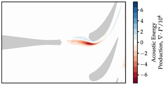
Figure 6.
Acoustic energy production in the combustor–turbine gap at mid-span of the Datum geometry, at reduced frequency . Loss is concentrated downstream of the combustor wall.
Acoustic loss by streamwise mean flow interaction is a distinct mechanism from interactions with combustor trailing edge vortex shedding. If trailing edge vortex shedding were dominant, the region of negative acoustic energy production would be located on the upstream side of the gap—loss by shedding is inconsistent with the contours in Figure 6. The shedding frequency is a factor of five higher than the acoustic frequency, so there is no interaction in this Datum geometry with a thin trailing edge.
5. Can Transfer Function Predictions
The previous section showed that, for representative can-annular combustors, the acoustic reactance between cans is close to the Rayleigh conductivity, and the acoustic resistance is approximately with a weak sensitivity to geometry, varying by up to over a wide variety of cases. This section compares full-annulus CFD results for can transfer functions of the Datum geometry against predictions from the analytical model. To calibrate the connection impedance, reactance is set to the Rayleigh value and resistance is set to the value extracted from a two-can computation.
Figure 7 illustrates the importance of both modelling can-to-can communication and allowing for acoustic resistance. Naïvely applying the plane-wave reflection coefficient at the trailing edge of the combustor can, discounting transmission to other cans, is in error by a factor of two compared to the can reflection coefficient . Setting for a pure Rayleigh conductivity model after von Saldern et al. [4] ignores acoustic resistance and over-predicts by up to 68%.
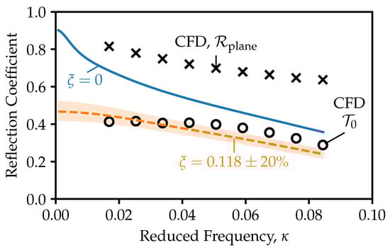
Figure 7.
Plane and can reflection coefficient magnitudes for Datum combustor, model (lines) and CFD (symbols). The Rayleigh conductivity model with over-predicts by up to 68%; using acoustic resistance extracted from a two-can simulation matches CFD to within 23%.
Using the resistance value extracted from a two-can computation of this geometry matches CFD to within 23% and is accurate to 8% at the compact reduced frequency . The shaded band in Figure 7 shows the sensitivity of predictions to the range of variation in observed across representative geometries with in Figure 4b. A perturbation in leads to a variation in —predicted can transfer function magnitudes are robust to inaccuracies in acoustic resistance.
Thermoacoustic stability of a can-annular ring of combustors depends on all can transfer functions . With the calibrated value of acoustic resistance , Figure 8 shows can transfer functions for as a function of reduced frequency. As k increases, transfer to more distant cans reduces, justifying a focus on small k (by symmetry ).
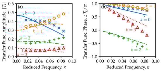
Figure 8.
Can transfer functions for Datum combustor: (a) magnitude, (b) phase. Comparison of analytical model (lines) to CFD simulations (symbols). With calibrated acoustic resistance , the analytical model agrees to within 0.03 magnitude at .
CFD computations and analytical model agree to within 0.03 magnitude at a low reduced frequency ; see Figure 8a. The gap is assumed compact in the analytical model, however, which results in first-order magnitude errors at high reduced frequencies . Compactness is the most fundamental and strongest assumption of the model. Accounting for non-compact effects would require a higher-fidelity two-dimensional solution of the acoustic field in the combustor–turbine gap. Phase predictions in Figure 8b agree to within 0.15rad at and qualitatively match the trend.
Figure 9 shows the effect of combustor–turbine gap length on can transfer functions. The assumption of compactness restricts the analysis to a low reduced frequency . The model quantitatively captures variations in the transfer functions, including a minimum near ; see Figure 9a. A constant acoustic resistance at the representative gap is sufficient to give good agreement across the range of gaps (the full results in Figure 5 are not used). If full-annulus computations at one gap length are available, fitting resistance a posteriori based on yields closer agreement, and the minima coincide between CFD and analytical model (results not shown).
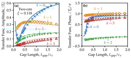
Figure 9.
Effect of combustor–turbine gap length on can transfer functions for Datum combustor at , model (lines) and CFD (symbols): (a) magnitude, (b) phase. Using one value of acoustic resistance calibrated at the datum gap, the model quantitatively captures the trends. A minimum occurs near .
Returning to Equation (6), the total impedance is given by turbine and combustor contributions in parallel. At a fixed frequency and azimuthal mode, there exists a value of where these two contributions align in destructive interference, giving a low total impedance. Although the can transfer functions are a combination of modal reflections (Equation (9)), the sharp phase shift of in Figure 9b near the inflection point supports this explanation for the existence of the minimum.
6. Design Space Study—Minimising Reflected Energy
Both the CFD simulations and analytical model identify in Figure 9 a minimum can reflection coefficient occurring at non-zero gap length. This section uses the analytical model to determine the parameters affecting this minimum and the implications for coupled combustor and turbine design.
Greatest thermoacoustic stability benefit corresponds to minimum reflected acoustic energy, calculated as With less reflected energy, the combustor requires less acoustic damping to maintain stability. Summing over all cans accounts for the fact that a minimum in just may correspond to redistribution of transmission to other cans, rather than increasing transmission through the turbine.
For the case presented in Figure 9, at the representative gap length the reflected energy takes a value . Reducing the gap length until a minimum is reached at , the reflected energy reduces to a low of , a 63% drop with respect to the representative gap.
The analytical model in Equation (6) contains four independent parameters:
Fixing the annulus mean radius and hub-to-tip radius ratio, and varying the number of cans, is one way to change . The choice of hub-to-tip ratio is arbitrary because both and are proportional to annulus height. In common with the predictions presented so far, acoustic reactance is set to the Rayleigh value, while the acoustic resistance is a free parameter. This design study assumes a constant reduced frequency, , in the compact regime where the analytical model is most accurate. The design study also assumes a real downstream reflection coefficient with no phase shift, a valid simplification in the compact regime.
Figure 10a illustrates the variation in gap length at minimum reflected energy, , when the remaining three non-dimensional parameters are perturbed away from a baseline condition representative of large industrial gas turbines. is inversely proportional to the number of cans. Because and , this corresponds to the minima occurring at a constant value of , when other parameters are fixed. Figure 10a also shows that is directly proportional to acoustic resistance and downstream turbine reflection coefficient.
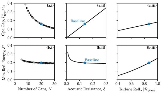
Figure 10.
Effect of design parameters (i) number of cans, N; (ii) acoustic resistance, ; and (iii) turbine reflection coefficient, on (a) optimum combustor–turbine gap length, (b) minimum reflected energy. Optimum gap length is inversely proportional to N and proportional to and .
Figure 10b plots the minimum reflected energy, , as a function of the parameters in Equation (14). The number of cans has a weak effect, with increasing by 21% as N drops from the datum 20 to 7. As acoustic resistance drops towards zero, rises rapidly—the existence of a minimum requires non-zero resistance and would not be captured by a pure Rayleigh conductivity model. Minimum reflected energy increases as the downstream turbine becomes more reflective, consistent with the parallel form of Equation (6).
The relationships in Figure 10a imply the optimum gap length corresponds to
where analytical modelling over the entire design space of Figure 10 has been used to calculate the constant, at a compact reduced frequency . Raising reduced frequency to increases the constant by 13%. Equation (15) is a design guideline that informs selection of the combustor–turbine gap for minimum reflection and maximum acoustic loss from the combustion system.
To use the guideline in practice, an engineer has several options for assigning an acoustic resistance. With no computations available, a first guess from past experience could be . A two-can computation of a novel geometry provides a more accurate resistance, and if necessary, reactance. Fitting to a full-annulus computation gives the most precise value for . Then, rearranging Equation (15) for and dividing by annulus height gives the optimum gap length.
7. Conclusions
This paper applied time-marching CFD and an analytical model to predict transfer functions between incident and reflected waves in a can-annular combustor. These transfer functions are necessary boundary conditions for a thermoacoustic model to determine stability of the combustion system. The results show:
- The connection impedance analytical model of von Saldern et al. [4] requires acoustic resistance of order for can transfer functions to match CFD simulations of a representative gas turbine combustor. The resistance arises due to streamwise mean flow and for representative combustor wall thicknesses is a weak function of combustor can geometry.
- With a calibrated acoustic resistance, the analytical model reproduces full-annulus CFD can transfer functions to within 0.03 amplitude and 0.15 rad phase in the compact regime, indicating validity of the modelling assumptions. Prediction errors increase rapidly for due to non-compact effects.
- As combustor–turbine gap length is varied, for a given compact frequency, there is a minimum reflected energy at a non-zero gap length. In the datum case, reflected energy drops by 63% at compared to the datum . The minimum, where contributions from downstream turbine and other cans align in antiphase, is captured by both CFD simulations and the analytical model.
- Analytical exploration of the coupled can-annular combustor–turbine design space yields a guideline for minimum reflected energy: at optimum gap length,
The present analytical model is shown to be a useful tool for estimating acoustic boundary conditions in a rapid, iterative combustor design process, subject to two limitations. First, the value of acoustic resistance must be calibrated; the transfer functions, however, are not strongly sensitive to this parameter. Second, the model assumes low reduced frequencies, which are typical of instability in large industrial machines but cannot be assumed in general. The mechanism of separate can and turbine impedance contributions resulting in an optimum gap length will remain at higher frequencies.
Funding
This research was funded by Mitsubishi Heavy Industries, grant number G106034.
Data Availability Statement
The author does not have permission to share data.
Acknowledgments
The author thanks Mitsubishi Heavy Industries for funding this project, in particular S. Uchida, K. Saitoh, and T. Koda for their interest and support. The author is grateful to G. Pullan for his comments on a draft of this manuscript.
Conflicts of Interest
The author declares no conflict of interest.
Nomenclature
| Roman | Greek | ||||
| a | [] | Acoustic wave speed | [–] | Specific heat ratio | |
| A | [] | Area | [–] | Reflected acoustic energy | |
| [] | Vane axial chord | [–] | Connection impedance | ||
| f | [] | Frequency | [–] | Acoustic reactance | |
| [–] | Imaginary unit | [] | Angular coordinate | ||
| k | [–] | Can offset index | [–] | Reduced frequency | |
| [] | Combustor–turbine gap | [] | Kinematic viscosity | ||
| m | [–] | Azimuthal mode index | [–] | Acoustic resistance | |
| n | [–] | Can index | [] | Density | |
| N | [–] | Number of cans | Subscripts and accents | ||
| p | [] | Pressure | 0 | Stagnation conditions | |
| [–] | Reflection coefficient | Characteristic wave | |||
| T | [] | Temperature | Perturbation relative to mean | ||
| [–] | Transmission coefficient | Upstream- or downstream-running | |||
| V | [] | Velocity | Azimuthal mode | ||
| w | [] | Combustor wall thickness | Time average | ||
| [–] | Non-dim’l. impedance | Minimum reflected acoustic energy | |||
References
- Kaufmann, P.; Krebs, W.; Valdes, R.; Wever, U. 3D Thermoacoustic Properties of Single Can and Multi Can Combustor Configurations. In Proceedings of the ASME Turbo Expo; ASME: New York, NY, USA, 2008. [Google Scholar] [CrossRef]
- Venkatesan, K.; Cross, A.; Yoon, C.; Han, F.; Bethke, S. Heavy Duty Gas Turbine Combustion Dynamics Study Using a Two-Can Combustion System. In Proceedings of the ASME Turbo Expo; ASME: New York, NY, USA, 2019. [Google Scholar] [CrossRef]
- Ghirardo, G.; Di Giovine, C.; Moeck, J.P.; Bothien, M.R. Thermoacoustics of Can-Annular Combustors. J. Eng. Gas Turbines Power 2019, 141, 011007. [Google Scholar] [CrossRef]
- von Saldern, J.G.R.; Orchini, A.; Moeck, J.P. Analysis of Thermoacoustic Modes in Can-Annular Combustors Using Effective Bloch-Type Boundary Conditions. J. Eng. Gas Turbines Power 2021, 143, 071019. [Google Scholar] [CrossRef]
- Fournier, G.J.J.; Meindl, M.; Silva, C.F.; Ghirardo, G.; Bothien, M.R.; Polifke, W. Low-Order Modeling of Can-Annular Combustors. J. Eng. Gas Turbines Power 2021, 143, 121004. [Google Scholar] [CrossRef]
- Brind, J. Acoustic Boundary Conditions for Can-Annular Combustors. In Proceedings of the 15th European Turbomachinery Conference, paper No. ETC2023-140, Budapest, Hungary, 24–28 April 2023. [Google Scholar]
- Orchini, A. An effective impedance for modelling the aeroacoustic coupling of ducts connected via apertures. J. Sound Vib. 2022, 520, 116622. [Google Scholar] [CrossRef]
- Brind, J.; Pullan, G. Modelling Turbine Acoustic Impedance. Int. J. Turbomach. Propuls. Power 2021, 6, 18. [Google Scholar] [CrossRef]
- Brandvik, T.; Pullan, G. An Accelerated 3D Navier–Stokes Solver for Flows in Turbomachines. J. Turbomach. 2011, 133, 021025. [Google Scholar] [CrossRef]
- Poinsot, T.; Le Chatelier, C.; Candel, S.; Esposito, E. Experimental determination of the reflection coefficient of a premixed flame in a duct. J. Sound Vib. 1986, 107, 265–278. [Google Scholar] [CrossRef]
- Miles, J.H. Acoustic transmission matrix of a variable area duct or nozzle carrying a compressible subsonic flow. J. Acoust. Soc. Am. 1981, 69, 1577–1586. [Google Scholar] [CrossRef]
- Miles, J.H. Author’s reply. J. Sound Vib. 1995, 182, 328–335. [Google Scholar] [CrossRef]
- Morfey, C. Acoustic energy in non-uniform flows. J. Sound Vib. 1971, 14, 159–170. [Google Scholar] [CrossRef]
Disclaimer/Publisher’s Note: The statements, opinions and data contained in all publications are solely those of the individual author(s) and contributor(s) and not of MDPI and/or the editor(s). MDPI and/or the editor(s) disclaim responsibility for any injury to people or property resulting from any ideas, methods, instructions or products referred to in the content. |
© 2023 by the author. Licensee MDPI, Basel, Switzerland. This article is an open access article distributed under the terms and conditions of the Creative Commons Attribution (CC BY-NC-ND) license (https://creativecommons.org/licenses/by-nc-nd/4.0/).