
Experimental Validation of a Numerical Coupling Environment Applying FEM and CFD †

 ,
,
Abstract
:1. Introduction
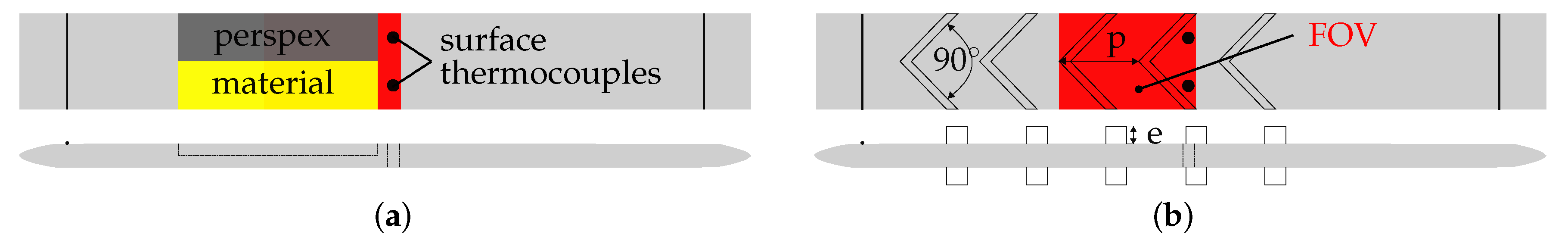
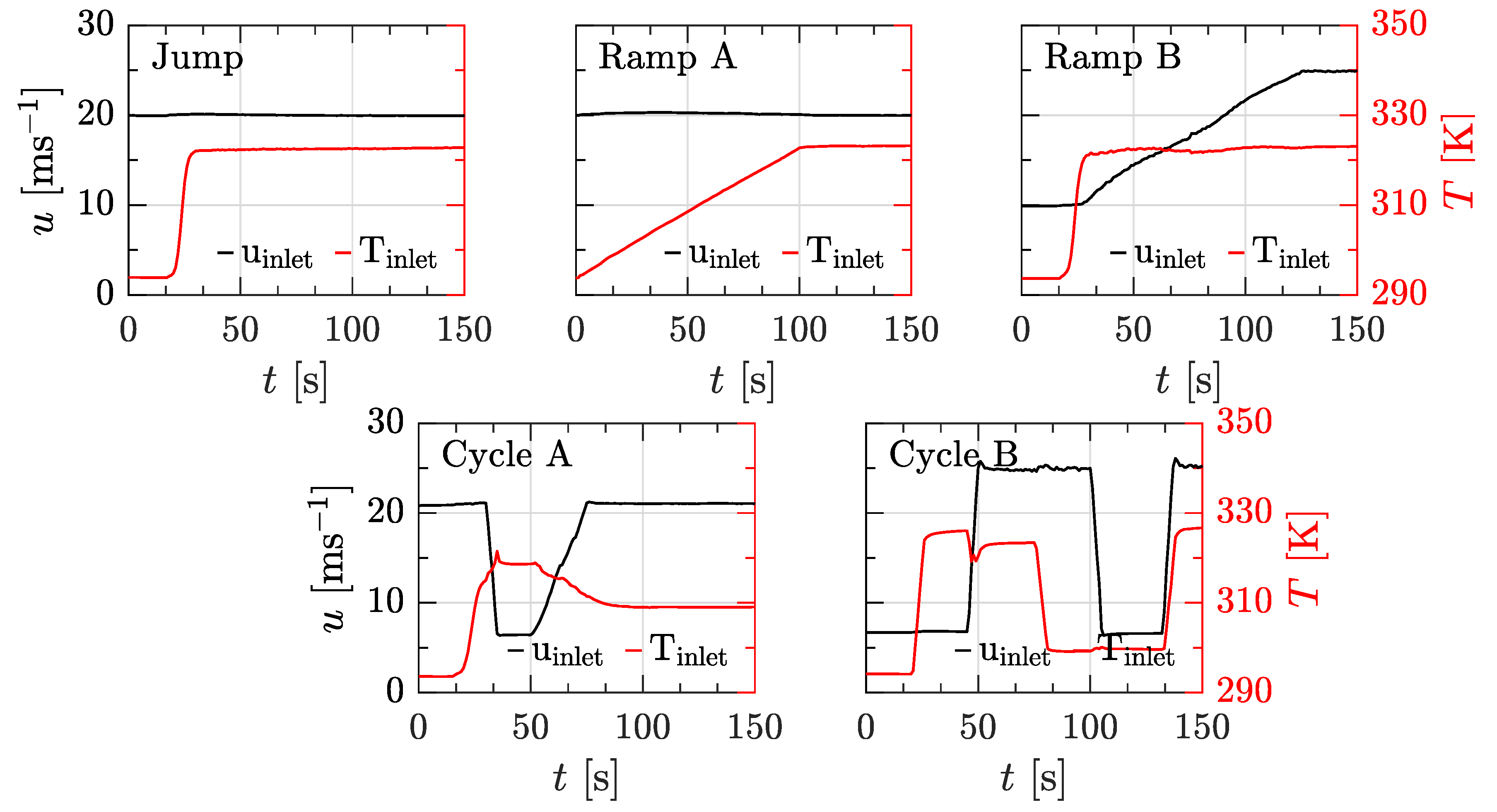
2. Experimental Setup
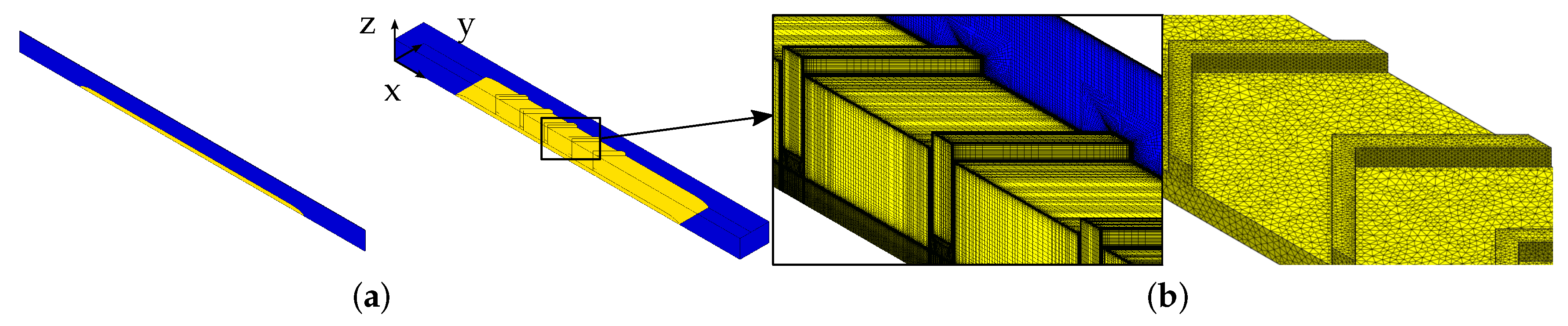
3. Numerical Setup
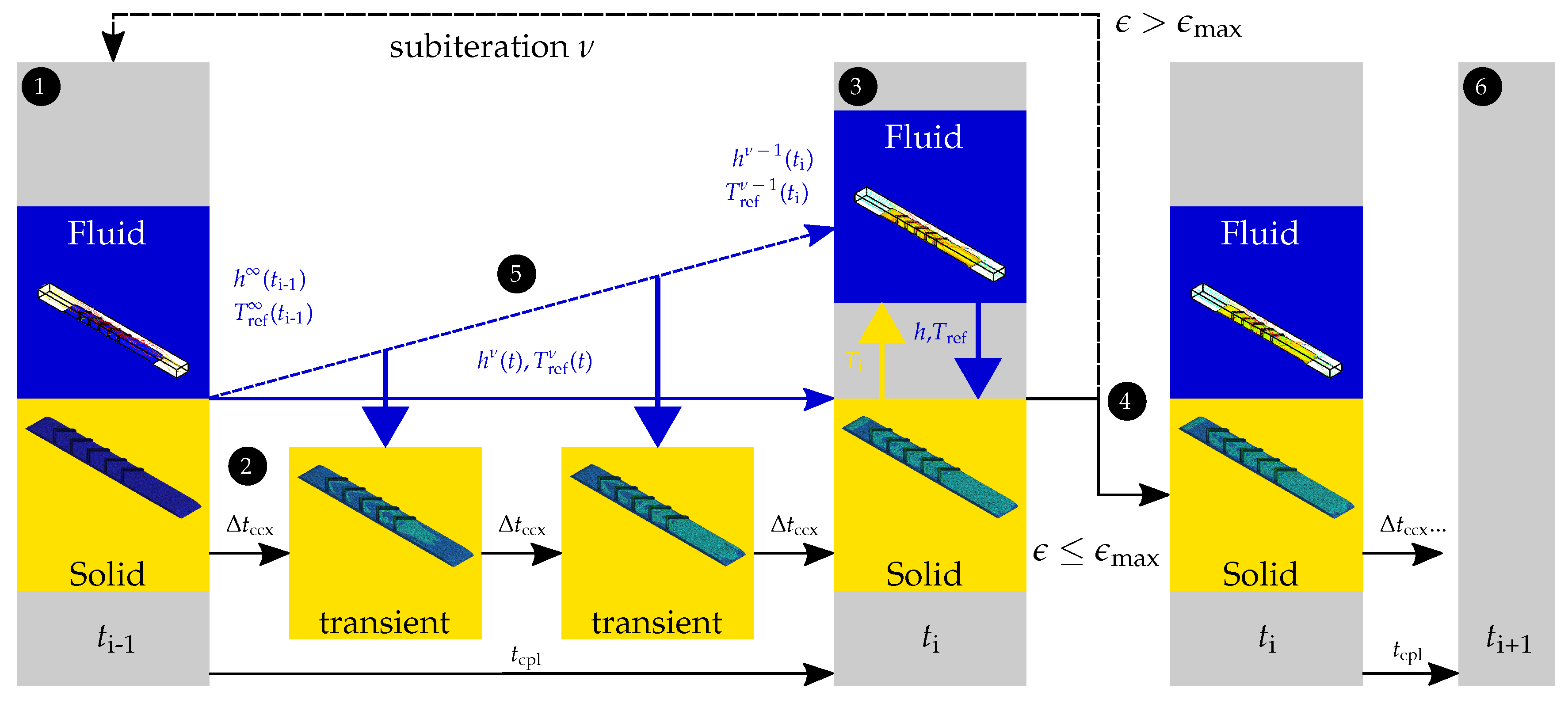
4. Coupling Environment
5. Data Reduction and Evaluation
6. Results
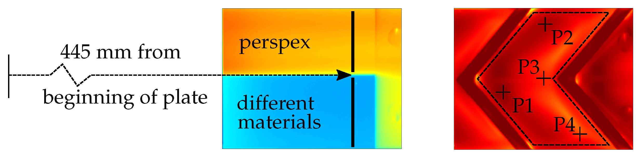
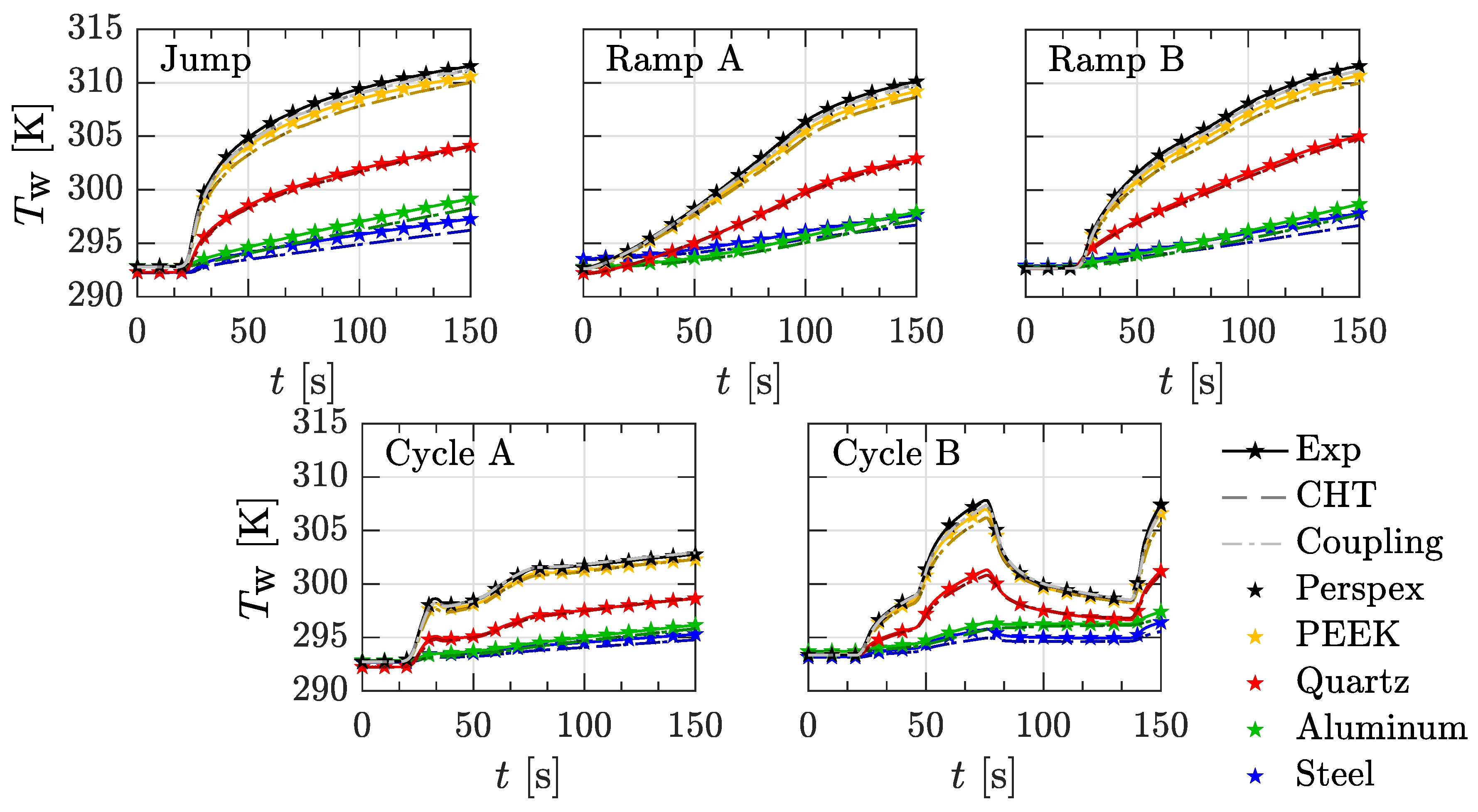
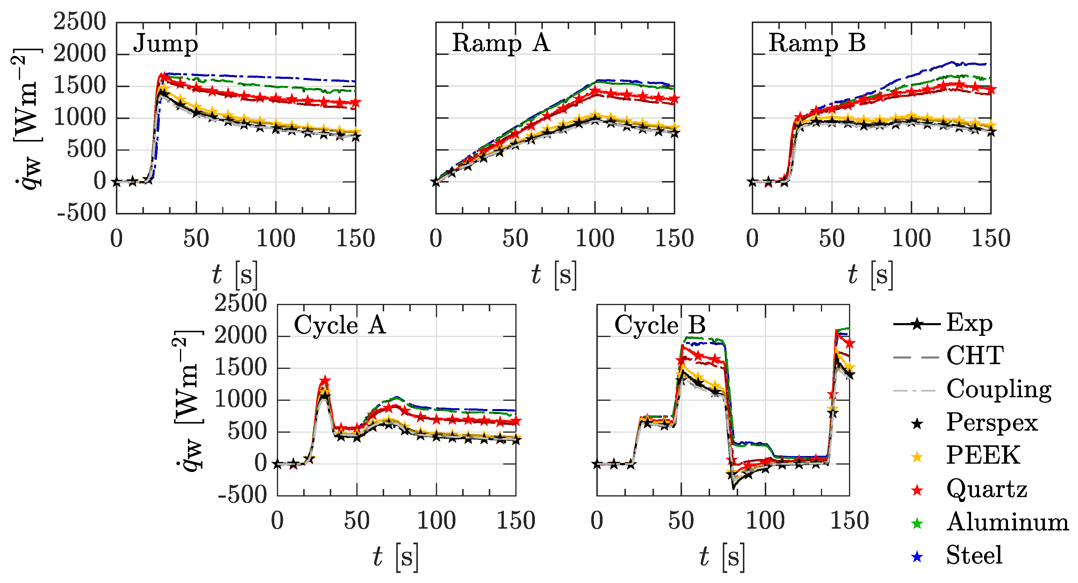
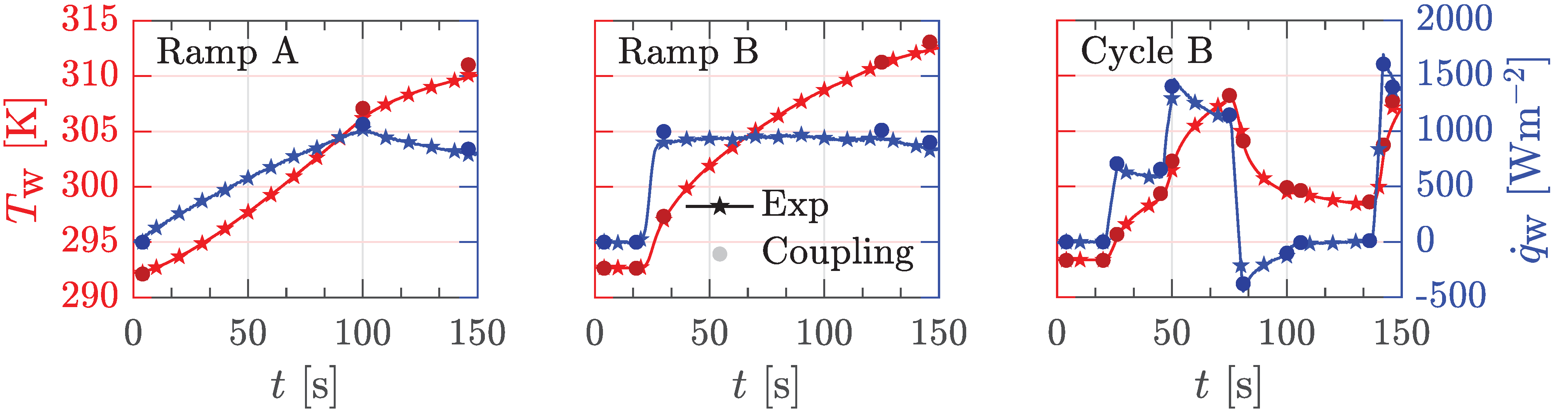
6.1. Flat Plate
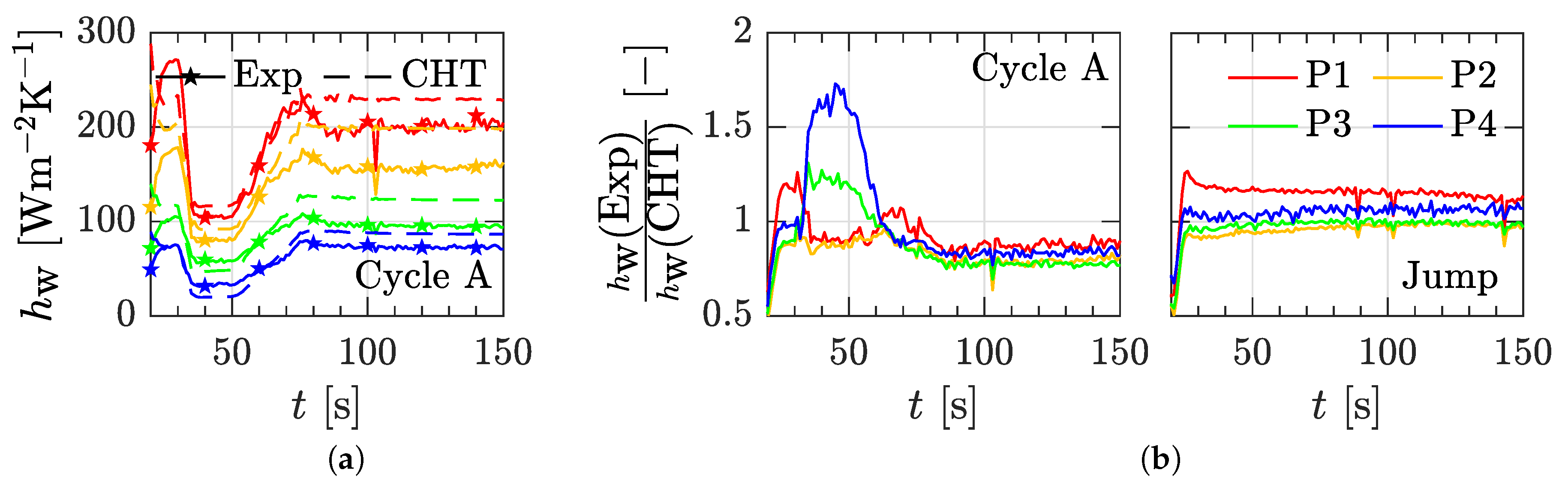
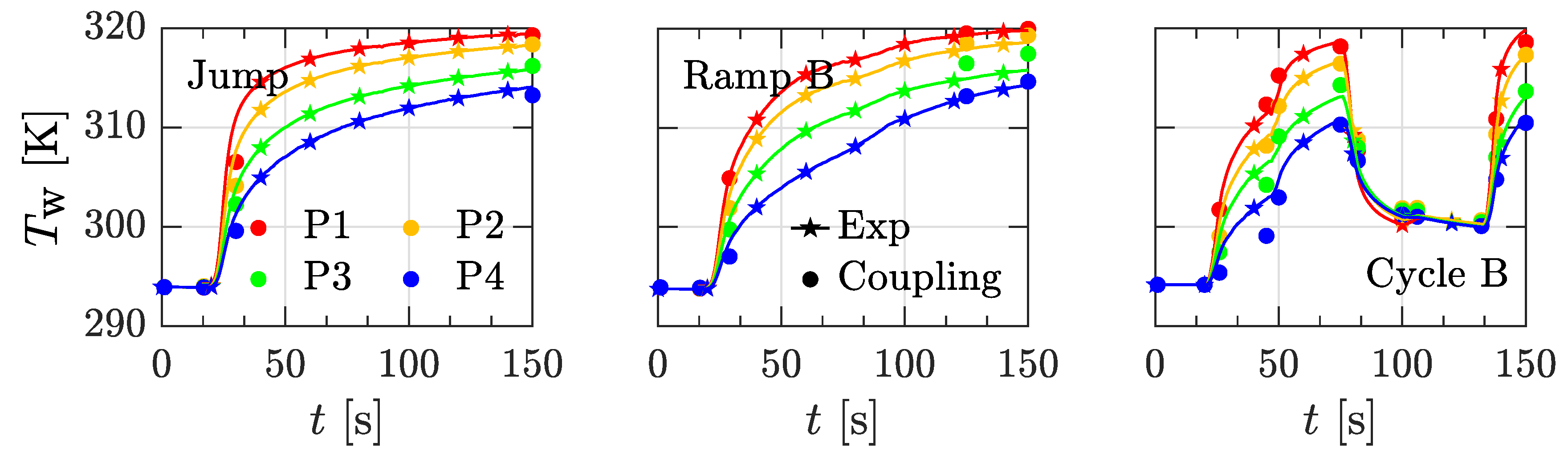
6.2. Plate with V-Shaped Ribs
7. Conclusions
Author Contributions
Funding
Institutional Review Board Statement
Informed Consent Statement
Data Availability Statement
Acknowledgments
Conflicts of Interest
Nomenclature and Abbreviations
| Roman characters | |
| specific heat capacity in | |
| e | characteristic rib height in |
| h | heat transfer coefficient in |
| i | index |
| k | thermal conductivity in |
| L | length in |
| p | pitch of ribs in |
| p | pressure in |
| heat flux in | |
| t | time in |
| T | temperature in |
| u | velocity in |
| coordinates in | |
| dimensionless wall distance | |
| Greek characters | |
| norm | |
| dynamic viscosity in | |
| subiteration number | |
| density in | |
| Subscripts | |
| ccx | CalculiX |
| cpl | coupling |
| ref | reference |
| w | wall |
| CCT | constant current thermometry |
| CFD | computational fluid dynamics |
| CHT | conjugate heat transfer |
| CTA | constant temperature anemometry |
| Exp | experiment |
| FEM | finite element method |
| FOV | field of view |
| FVM | finite volume method |
| IRT | infrared thermography |
| SST | shear stress transport |
References
- Perelman, T. On conjugated problems of heat transfer. Int. J. Heat Mass Transf. 1961, 3, 293–303. [Google Scholar] [CrossRef]
- Fiedler, B.; Muller, Y.; Voigt, M.; Mailach, R. Comparison of Two Methods for the Sensitivity Analysis of a One-Dimensional Cooling Flow Network of a High-Pressure-Turbine Blade. In Volume 2D: Turbomachinery; American Society of Mechanical Engineers: New York, NY, USA, 2020. [Google Scholar] [CrossRef]
- Heselhaus, A.; Vogel, D. Numerical simulation of turbine blade cooling with respect to blade heat conduction and inlet temperature profiles. In Proceedings of the 31st Joint Propulsion Conference and Exhibit, San Diego, CA, USA, 10–12 July 1995. [Google Scholar] [CrossRef]
- Felippa, C.A.; Park, K.; Farhat, C. Partitioned analysis of coupled mechanical systems. Comput. Methods Appl. Mech. Eng. 2001, 190, 3247–3270. [Google Scholar] [CrossRef]
- Sun, Z.; Chew, J.W.; Hills, N.J.; Lewis, L.; Mabilat, C. Coupled Aerothermomechanical Simulation for a Turbine Disk Through a Full Transient Cycle. J. Turbomach. 2011, 134, 011014. [Google Scholar] [CrossRef]
- Amirante, D.; Hills, N.J.; Barnes, C.J. Thermo-Mechanical Finite Element Analysis/Computational Fluid Dynamics Coupling of an Interstage Seal Cavity Using Torsional Spring Analogy. J. Turbomach. 2012, 134, 051015. [Google Scholar] [CrossRef]
- He, L.; Oldfield, M.L.G. Unsteady Conjugate Heat Transfer Modeling. J. Turbomach. 2010, 133, 031022. [Google Scholar] [CrossRef]
- Errera, M.P.; Baqué, B. A quasi-dynamic procedure for coupled thermal simulations. Int. J. Numer. Methods Fluids 2013, 72, 1183–1206. [Google Scholar] [CrossRef]
- Errera, M.P.; Duchaine, F. Comparative study of coupling coefficients in Dirichlet–Robin procedure for fluid–structure aerothermal simulations. J. Comput. Phys. 2016, 312, 218–234. [Google Scholar] [CrossRef]
- Gimenez, G.; Errera, M.P.; Baillis, D.; Smith, Y.; Pardo, F. A coupling numerical methodology for weakly transient conjugate heat transfer problems. Int. J. Heat Mass Transf. 2016, 97, 975–989. [Google Scholar] [CrossRef]
- Khoury, R.R.E.; Errera, M.P.; Khoury, K.E.; Nemer, M. Efficiency of coupling schemes for the treatment of steady state fluid-structure thermal interactions. Int. J. Therm. Sci. 2017, 115, 225–235. [Google Scholar] [CrossRef]
- Moretti, R.; Errera, M.P.; Feyel, F. Temporal Interpolation Methods for Transient CHT. In Proceedings of the AIAA Scitech 2019 Forum, San Diego, CA, USA, 7–11 January 2019; American Institute of Aeronautics and Astronautics: Reston, VI, USA, 2019. [Google Scholar] [CrossRef]
- Verstraete, T.; Scholl, S. Stability analysis of partitioned methods for predicting conjugate heat transfer. Int. J. Heat Mass Transf. 2016, 101, 852–869. [Google Scholar] [CrossRef]
- Sun, Z.; Chew, J.; Hills, N.; Volkov, K.; Barnes, C. Efficient Finite Element Analysis/Computational Fluid Dynamics Thermal Coupling for Engineering Applications. J. Turbomach. 2010, 132, 031016. [Google Scholar] [CrossRef]
- Verdicchio, J.A.; Chew, J.W.; Hills, N.J. Coupled Fluid/Solid Heat Transfer Computation for Turbine Discs. In Volume 3: Heat Transfer; Electric Power; Industrial and Cogeneration; American Society of Mechanical Engineers: New York, NY, USA, 2001. [Google Scholar] [CrossRef]
- Dixon, J.A.; Valencia, A.G.; Coren, D.; Eastwood, D.; Long, C. Main Annulus Gas Path Interactions—Turbine Stator Well Heat Transfer. J. Turbomach. 2013, 136, 021010. [Google Scholar] [CrossRef]
- Ganine, V.; Javiya, U.; Hills, N.; Chew, J. Coupled Fluid-Structure Transient Thermal Analysis of a Gas Turbine Internal Air System With Multiple Cavities. J. Eng. Gas Turbines Power 2012, 134, 102508. [Google Scholar] [CrossRef]
- Schindler, A.P.; Brack, S.; von Wolfersdorf, J. Coupled FE-CFD analysis of transient conjugate heat transfer. In Proceedings of the 13th European Conference on Turbomachinery Fluid Dynamics and Thermodynamics, Lausanne, Switzerland, 8–12 April 2019. [Google Scholar] [CrossRef]
- Dhondt, G. The Finite Element Method for Three-Dimensional Thermomechanical Applications; Wiley: Hoboken, NJ, USA, 2004. [Google Scholar]
- Estorf, M. Image based heating rate calculation from thermographic data considering lateral heat conduction. Int. J. Heat Mass Transf. 2006, 49, 2545–2556. [Google Scholar] [CrossRef]
- Israel, U.; Cottier, F.; Hartmann, C.; von Wolfersdorf, J. Method for transient and steady state partitioned fluid-structure interaction analysis in conjugate heat transfer for aero engines applications. In Proceedings of the 15th European Conference on Turbomachinery Fluid Dynamics and Thermodynamics, Budapest, Hungary, 24–28 April 2023. [Google Scholar] [CrossRef]
- Hartmann, C.; Schweikert, J.; Cottier, F.; Israel, U.; Gier, J.; von Wolfersdorf, J. Experimental Validation of a Numerical Coupling Environment between FEM and CFD. In Proceedings of the 15th European Conference on Turbomachinery Fluid Dynamics and Thermodynamics, Budapest, Hungary, 24–28 April 2023. [Google Scholar] [CrossRef]
- Liu, C.; von Wolfersdorf, J.; Zhai, Y. Time-resolved heat transfer characteristics for steady turbulent flow with step changing and periodically pulsating flow temperatures. Int. J. Heat Mass Transf. 2014, 76, 184–198. [Google Scholar] [CrossRef]
- Brack, S.; Poser, R.; von Wolfersdorf, J. Experimental investigation of unsteady convective heat transfer under airflow velocity and temperature variations. Meas. Sci. Technol. 2021, 33, 015106. [Google Scholar] [CrossRef]
- Menter, F.R. Two-equation eddy-viscosity turbulence models for engineering applications. AIAA J. 1994, 32, 1598–1605. [Google Scholar] [CrossRef]
- Menter, F.R.; Kuntz, M.; Langtry, R. Ten years of industrial experience with the SST turbulence model. Heat Mass Transf. 2003, 4, 625–632. [Google Scholar]
- Göhring, M.; Krille, T.; Feile, J.; von Wolfersdorf, J. Heat Transfer Predictions in Smooth and Ribbed Two-Pass Cooling Channels under Stationary and Rotating Conditions. In Proceedings of the 16th International Symposium on Transport Phenomena and Dynamics of Rotating Machinery, Honolulu, HI, USA, 10–15 April 2016; Available online: https://hal.archives-ouvertes.fr/hal-01884254 (accessed on 13 April 2021).
- Sutherland, W. LII. The viscosity of gases and molecular force. Lond. Edinb. Dublin Philos. Mag. J. Sci. 1893, 36, 507–531. [Google Scholar] [CrossRef]
- White, F. Viscous Fluid Flow; McGraw-Hill Higher Education: New York, NY, USA, 2006. [Google Scholar]
- Cottier, F.; Pinchaud, P.; Dumas, G. Aerothermal predictions of combustor/turbine interactions using advanced turbulence modeling. In Proceedings of the 13th European Conference on Turbomachinery Fluid Dynamics and Thermodynamics, Lausanne, Switzerland, 8–12 April 2019. [Google Scholar] [CrossRef]
- Aitken, A.C. On Bernoulli’s Numerical Solution of Algebraic Equations. Proc. R. Soc. Edinb. 1927, 46, 289–305. [Google Scholar] [CrossRef]
- Vogel, G.; Weigand, B. A new evaluation method for transient liquid crystal experiments. In Proceedings of the 2001 National Heat Transfer Conference, ASME, Anaheim, CA, USA, 10–12 June 2001. [Google Scholar]
- Wagner, G.; Kotulla, M.; Ott, P.; Weigand, B.; von Wolfersdorf, J. The Transient Liquid Crystal Technique: Influence of Surface Curvature and Finite Wall Thickness. J. Turbomach. 2005, 127, 175–182. [Google Scholar] [CrossRef]
- Kays, W.; Crawford, M.; Weigand, B. Convective Heat and Mass Transfer; McGraw-Hill Series in Mechanical Engineering: New York, NY, USA, 2005; Volume 30. [Google Scholar]
- Moffat, R.J. Contributions to the Theory of Single-Sample Uncertainty Analysis. J. Fluids Eng. 1982, 104, 250–258. [Google Scholar] [CrossRef]
- Esfahani, J.A.; Jafarian, M.M. Entropy Generation Analysis of a Flat Plate Boundary Layer with Various Solution Methods. Sci. Iran. 2005, 12, 233–240. [Google Scholar]
- Herwig, H. The Role of Entropy Generation in Momentum and Heat Transfer. J. Heat Transf. 2012, 134, 031003. [Google Scholar] [CrossRef]


| Perspex | PEEK | Quartz | Steel | Aluminum | |
|---|---|---|---|---|---|
| 1190 | 1310 | 2200 | 7900 | 2700 | |
| 1470 | 1340 | 670 | 500 | 888 | |
| 0.19 | 0.25 | 1.4 | 15 | 237 |
| Approach | Test Case | Material | |||||||||||
|---|---|---|---|---|---|---|---|---|---|---|---|---|---|
| Geometry | E | C | C | Ramp | Cycle | Perspex | PEEK | Quartz | Aluminium | Steel | |||
| x | H | p | Jump | A | B | A | B | ||||||
| p | T | l | |||||||||||
| Flat plate | X | X | X | X | X | X | X | X | X | X | X | X | X |
| V-ribs | X | X | X | X | X | X | X | X | X | ||||
| Perspex | PEEK | Quartz | Steel | Aluminum | |
|---|---|---|---|---|---|
| 517.9 | 395.0 | 59.2 | 14.8 | 0.6 | |
| Bi | 4.7 | 3.6 | 0.64 | 0.06 | 0.0038 |
Disclaimer/Publisher’s Note: The statements, opinions and data contained in all publications are solely those of the individual author(s) and contributor(s) and not of MDPI and/or the editor(s). MDPI and/or the editor(s) disclaim responsibility for any injury to people or property resulting from any ideas, methods, instructions or products referred to in the content. |
© 2023 by the authors. Licensee MDPI, Basel, Switzerland. This article is an open access article distributed under the terms and conditions of the Creative Commons Attribution (CC BY-NC-ND) license (https://creativecommons.org/licenses/by-nc-nd/4.0/).
Share and Cite
Hartmann, C.; Schweikert, J.; Cottier, F.; Israel, U.; Gier, J.; von Wolfersdorf, J. Experimental Validation of a Numerical Coupling Environment Applying FEM and CFD. Int. J. Turbomach. Propuls. Power 2023, 8, 31. https://doi.org/10.3390/ijtpp8030031
Hartmann C, Schweikert J, Cottier F, Israel U, Gier J, von Wolfersdorf J. Experimental Validation of a Numerical Coupling Environment Applying FEM and CFD. International Journal of Turbomachinery, Propulsion and Power. 2023; 8(3):31. https://doi.org/10.3390/ijtpp8030031
Chicago/Turabian StyleHartmann, Christopher, Julia Schweikert, François Cottier, Ute Israel, Jochen Gier, and Jens von Wolfersdorf. 2023. "Experimental Validation of a Numerical Coupling Environment Applying FEM and CFD" International Journal of Turbomachinery, Propulsion and Power 8, no. 3: 31. https://doi.org/10.3390/ijtpp8030031
APA StyleHartmann, C., Schweikert, J., Cottier, F., Israel, U., Gier, J., & von Wolfersdorf, J. (2023). Experimental Validation of a Numerical Coupling Environment Applying FEM and CFD. International Journal of Turbomachinery, Propulsion and Power, 8(3), 31. https://doi.org/10.3390/ijtpp8030031