Article

Machine Learning Based Sensitivity Analysis of Aeroelastic Stability Parameters in a Compressor Cascade †

Department of Mechanical Engineering, Imperial College London, London SW7 2AZ, UK
*
Author to whom correspondence should be addressed.
This paper is a revised version of our paper published in Proceedings of the European Turbomachinery Conference ETC14, Gdansk, Poland, 12–16 April 2021.
Int. J. Turbomach. Propuls. Power 2021, 6(3), 39; https://doi.org/10.3390/ijtpp6030039
Submission received: 19 May 2021 / Revised: 1 September 2021 / Accepted: 7 September 2021 / Published: 15 September 2021

Abstract

:
Aeroelastic instabilities such as flutter have a crucial role in limiting the operating range and reliability of turbomachinery. This paper offers an alternative approach to aeroelastic analysis, where the sensitivity of aerodynamic damping with respect to main flow and structural parameters is quantified through a surrogate-model-based investigation. The parameters are chosen based on previous studies and are represented by a uniform distribution within applicable intervals. The surrogate model is an artificial neural network, trained and tested to achieve an error within 1% of the test data. The quantity of interest is aerodynamic damping and the datasets are obtained from a linearised aeroelastic solver. The sensitivity of aerodynamic damping with respect to the input variables is obtained by calculating normalised gradients from the surrogate model at specific operating conditions. The results show a quantitative comparison of sensitivity across the different input parameters. The outcome of the sensitivity analysis is then used to decide the most appropriate action to take in order to induce stability in unstable operating conditions. The work is a preliminary study, carried out on a simplified two dimensional compressor cascade and it is aimed at proving the validity of a data-driven approach in studying the aeroelastic behaviour of turbomachinery. To the best of the authors’ knowledge, this is the first time a data-driven flutter model has been investigated. The initial results are encouraging, indicating that this approach is worth pursuing in the future. The presented framework can be used as a redesign tool to enhance the flutter stability of an existing blade.

1. Introduction

The development of highly loaded, three-dimensional, long compressor and fan blades yields a great challenge in terms of aeroelastic stability of turbomachinery. The task of assessing blade stability is only made more compelling by the recent trend towards blisks, in which mechanical damping is hardly present. Self-excited vibration, or flutter, is among the several aeroelastic phenomena which can limit the operating range of turbomachinery and eventually lead to blade failure. Flutter has been extensively studied by several authors, through analytical, experimental and computational methods, leading to a wealth of literature in which several driving parameters have been identified [1,2,3]. In [4], Srinivasan associates flutter with high steady loading and low reduced frequency, for blades vibrating in first bending or twist modes. The reduced frequency is addressed here as k = ω c / U r e l , where ω is the angular vibration frequency, c is the blade chord and U r e l is the inlet relative flow velocity. In an early analytical work [5], Whitehead presents unsteady lift calculations for a two-dimensional cascade of flat plates, emphasising that stability is affected, in different fashions depending on the flow variables (e.g., inlet Mach number), by the nature (cut-on waves propagate without attenuation, whereas cut-off waves decay as they travel) of acoustic waves produced by the vibration. The strong correlation between mean flow incidence and stability is shown in [6], using results from a complete analytical model for loaded cascades in incompressible flow developed in [7]. All of the above claims are corroborated by more recent computational studies. In [8], Vahdati and Cumpsty performed a three-dimensional CFD analysis of a state-of-the-art fan blade, and observed that (1) 3D separation (high loading), followed by radial migration of flow along the span towards the casing, reduces aerodynamic damping; (2) flutter occurs in the frequency and nodal diameter range where the generated acoustic waves are cut-on upstream and cut-off downstream (for an exhaustive explanation of acoustic modes in turbomachinery ducts see [9]); (3) aerodynamic damping decreases as the twist component in the first flap mode increases, in agreement with the study on turbines in [10]. Flutter is, therefore, influenced by steady and unsteady flow features, aeroacoustics and structural properties.
At early design stages, most of the attention is focused on performance, while aeroelastic stability is investigated only in terms of simple parameters such as reduced frequency. The influence of flow variables and other structural parameters is assessed only later in the process, or when in-service failure occurs. Although recent CFD-based methods have been successful in predicting flutter [11], the condition at which flutter occurs is unknown at the design stage; if unsteady CFD is to be used for such analysis, it can be very computationally expensive and cannot be used routinely. Moreover, given a specified range of design parameters variability, it is unclear in what measure these variables influence stability and how they quantitatively compare to one another. For example, is blade stiffening as effective as changing bending-twist ratio or the design point aerodynamics? How do flow features influence stability in different acoustic waves regimes?
The present paper will focus on the instability commonly known as stall flutter, which occurs at part-speed regime, when airfoils operate at an incidence higher than nominal [12]. It is misleadingly named so, since stall is not a necessary condition for its occurrence (Isomura and Giles [13] reported shock oscillations as instability exciting mechanism for their case, yet they referred to it as stall flutter). Inspired by the recent success of machine-learning-based uncertainty quantification of turbulence model coefficients [14,15,16], this paper attempts to answer the previous questions by means of a forward-propagation sensitivity analysis of selected design parameters, based on a machine-learnt surrogate model. The proposed method represents an alternative approach to current numerical stall flutter predictions which rely on ever growing computational methods [11,17]. The successful development of the proposed strategy would provide significant improvement over current CFD-based methods, as it requires significantly less computational resources. In addition, the machine-learnt model can provide quantitative measures of sensitivity, in the form of gradients of aerodynamic damping with respect to design parameters, offering optimum remedies for flutter issues of an existing design.
In this work, a simplified geometry is used to demonstrate the validity of a machine-learning-based framework to study the impact of flow and structural parameters on aerodynamic damping. The objective of the present work is to develop a redesign tool to enhance the flutter stability of an existing blade. The long term goal is to develop a simple model to assess stability of compressor and fan blades in order to provide early design guidelines focused on improving aeroelastic stability.
In the following sections, the choice of input coefficients, with their relative ranges, will be explained. Flow solver, machine learning model and forward-propagation strategy will be discussed and, finally, the results will be presented.

2. Methodology

2.1. Test Case

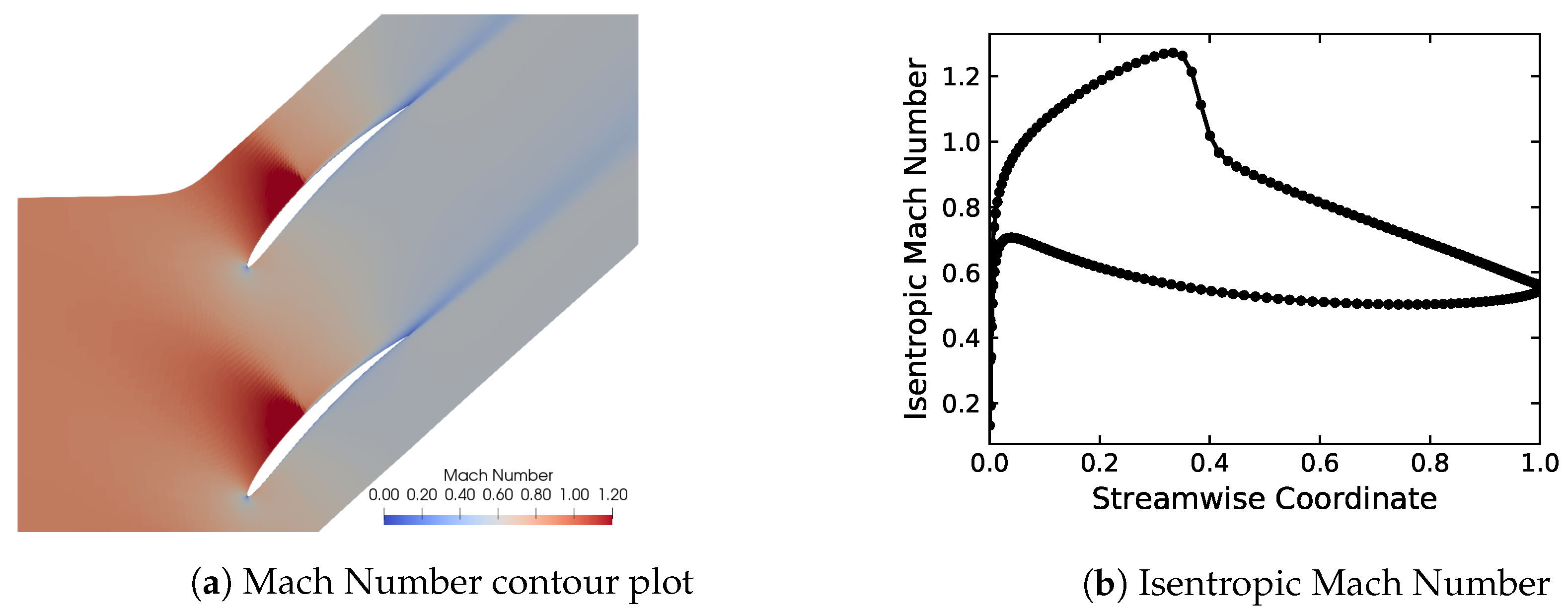
The test case selected for this study is the Standard Configuration 10 [18], a 2D compressor cascade. The chord length and pitch to chord ratio are fixed at 0.1 m and 1.0, respectively; the stagger angle is 45 ; inlet total pressure and temperature are 101.3 kPa and 300 K throughout the study and finally, at design point, the cascade operates with inlet Mach number M 1 = 0.7 and inflow angle α 1 = 55 . The incidence angle of flow onto the blade is referred to as β 1 , with β 1 = 0 corresponding to α 1 = 55 , and therefore to nominal incidence. Figure 1 shows an example of a steady state solution with M 1 = 0.85 and nominal incidence. The choice of a 2D geometry preserves the driving physics of flutter apart from two effects: three-dimensional flow profiles and presence of radial acoustic modes in the duct. Although relevant, these are not considered essential in the early design stage this work is targeting; moreover, this approach decouples the influence of tip leakage flow, which represents a cumbersome turbulence modelling problem in its own merit. Three-dimensional flow features will be included in future work.

2.2. Flow Solver

The CFD solver used in this work, LUFT, is developed by Dr. Paul Petrie-Repar from RPMTurbo. LUFT steady-state solver solves the 3D RANS equations on a hexahedral mesh, using a cell-centered finite volume scheme. The fluxes are calculated with an upwind Roe scheme (other schemes are available), the flow is reconstructed using a MUSCL interpolation with van Albada limiter and a local time stepping with residual smoothing is applied. The unsteady flow solver is linearised, casting the URANS equations in the frequency domain and the calculated unsteady pressures are used to evaluate aerodynamic work on the blade and subsequently aerodynamic damping, ζ . A linearised Spalart-Allmaras turbulence model is adopted, with no wall functions. Two-dimensional non-reflecting boundary conditions are applied throughout the study. The solver has been validated against other established codes [19,20].

2.3. Selection of Design Parameters

The relevant parameters chosen for this work are based on the literature presented in the previous section: inlet Mach number, M 1 , incidence angle, β 1 , reduced frequency k, bending-twist ratio of modeshape and Interblade Phase Angle, σ .
β 1 is imposed as boundary condition, M 1 is varied by changing the pressure ratio (inlet total pressure over outlet static pressure) across the cascade, k is imposed in the unsteady solver which, in turn, calculates the correct structural frequency using the steady state inlet flow velocity as reference. σ is specified in degrees and imposed as phase lag at the passage interfaces in the unsteady solver. The bending-twist ratio requires a little discussion.
The modeshape chosen for this work is a rigid body rotation about a given axis, referred to as twist axis. The bending-twist ratio is varied by keeping a fixed leading edge displacement, while changing the parameter X t , defined as:
X t = X L E + X T E X L E X T E
where X L E , X T E are signed leading and trailing edge displacements, respectively. The limiting cases are pure twist with X t = 0 and pure bending with X t ( X L E X T E ); all other cases, i.e., X t ( 0 , ) , are referred to as flap mode. The effect of increasing X t is, essentially, to move the twist axis further downstream from the blade (e.g., X t = 2 locates the twist axis half a chord away from the trailing edge); therefore, decreasing the twist component of the modeshape. Figure 2 shows a schematic illustration of the effect of increasing X t .
The next step is to decide the intervals in which the input parameters will vary. The interval for inlet Mach number is chosen to be symmetric about the nominal value of 0.7 , to study both subsonic flow, where no shock appears, and transonic flow conditions, where a shock is present on the suction side. M 1 , thus, changes between 0.5 , anything lower is discarded as excessively low speed, and 0.9 , so that the shock stays on the suction side and does not move too far upstream (Figure 1a). The incidence of incoming flow onto the blade is varied between 0 and 6 , which is the largest value before inception of stall for all the Mach numbers studied in this work. σ ranges from 180 to 180 ; the extremes are the same point, although no special treatment has been specified for them in the training phase of the surrogate model. In practice, the combination of reduced frequency and modeshape is not arbitrary: the same blade will be characterised by very different reduced frequencies whether it is vibrating in a pure twist or in a flap mode. Moreover, this combination also depends on the machine being considered: the flap mode of a fan blade will have a lower reduced frequency [17,21] compared to an embedded compressor blade [22]. Nevertheless, to cover the whole spectrum of combinations, modeshape and frequency in this study are assumed to be independent from each other during training of the surrogate model and, therefore, take large intervals. Table 1 summarises the space of input variables.

2.4. Sensitivity Analysis Method

The sensitivity analysis in this work is carried out by means of a surrogate model-based approach, in order to alleviate the computational load required by a conventional CFD-based method.
The Latin Hypercube sampling method [23] is applied to generate five independent databases of input parameters within the range in Table 1: this approach ensures a uniform distribution of the samples in the space of interest and that arbitrary samples from different databases are mutually independent. The databases have size 128, 256, 512, 1024, 2048, and are referred to as db1 to db5. The databases are applied to train and test a surrogate model of the CFD solver which will approximate aerodynamic damping without solving the aeroelastic equations:
q q ^ = S ( x )
where x is the input parameters vector, S is the surrogate model, q ^ and q are the quantity of interest, predicted by the surrogate model and CFD, respectively.
Finally, the PDF (probability density function) of aerodynamic damping can be obtained. The sensitivity of input coefficients on the prediction is quantified by the normalised gradient computed by the surrogate model, which will be briefly discussed.
The surrogate model S is a nonlinear function which given an input x R d outputs q ^ R m ; the Jacobian of the outputs with respect to input is:
J i j ( x ) = S i ( x ) x j = S i ( x )
The value of S i ( x ) will give a measure of how sensitive the output i is to the input j in the vicinity of x. In order to have a comparison between the inputs and across different locations of the sample space, the gradient is normalised by its magnitude | S i ( x ) | , yielding the normalised gradient.

2.5. Artificial Neural Network Based Surrogate Model

The artificial neural network (ANN) is used as a surrogate model of the CFD solver. The ANN is composed of multiple layers of nonlinear activation units called neurons. The input, hidden and output layers store input variables, intermediate outputs and quantity of interest, respectively. The vector of input variables x and quantity of interest q are below:
x = [ M 1 , β 1 , k , X t , σ ] q = ζ
The principles, training strategy and results are the following.

2.5.1. Forward Propagation

The input variables are normalised by their maximum and minimum and then rescaled in the range { 1 , 1 } :
a i ( 0 ) = 2 x i m i n ( x i ) m a x ( x i ) m i n ( x i ) 1
where x i is the vector of input variable i, with dimension m, where m is the number of samples. The outputs at intermediate layers are propagated as below:
a ( l + 1 ) = f ( z ( l + 1 ) ) = f ( w ( l + 1 ) a ( l ) + b ( l + 1 ) )
where w is the weights matrix, b = d i a g ( I ) is the bias vector and f ( · ) is the activation function. The function f ( x ) = A t a n h ( H x ) with A = 1.7159 and H = 2 3 is a rescaled hyperbolic tangent as proposed by [24]. The results at the output layer ( L + 1 ) are then denormalised to yield the quantity of interest:
q ^ = ( m a x ( q ) m i n ( q ) ) · a ( L + 1 ) + A 2 A + m i n ( q )
The max-min normalisation of the aerodynamic damping is symmetric with respect to zero so that | q ^ | q ^ = | ζ | ζ , i.e., negative q ^ (output of ANN) corresponds to negative aerodynamic damping. Lastly, the accuracy of ANN predictions is measured by the relative error on the test database:
ε = 1 m j = 1 m | q j q ^ j | m a x ( q ) m i n ( q )

2.5.2. Backpropagation

The ANN solves an optimisation problem by iteratively updating the weights w that connect the neurons. These are initialised randomly and are updated by minimising the cost function J:
J ( w , b ) = 1 2 m j = 1 m ( q j q ^ j ) 2 + λ 2 m l = 1 L + 1 ( w ( l ) ) 2
where λ regularises the weights norm so to avoid overfitting. The optimiser used in this work is the Broyden–Fletcher–Goldfarb–Shanno (BFGS, [25]). The gradient of the cost function is calculated as:
J w ( l ) = 1 m j = 1 m Δ ( l ) · ( a ( l 1 ) ) T + λ 2 m w ( l ) J b ( l ) = 1 m j = 1 m Δ ( l )
where:
Δ ( l ) = ( a ^ ( l ) a ( l ) ) · f ( z ( l ) ) , l = L + 1 ( w ( l + 1 ) ) T Δ ( l + 1 ) · f ( z ( l ) ) , 1 l L

2.5.3. Choice of Hyperparameters

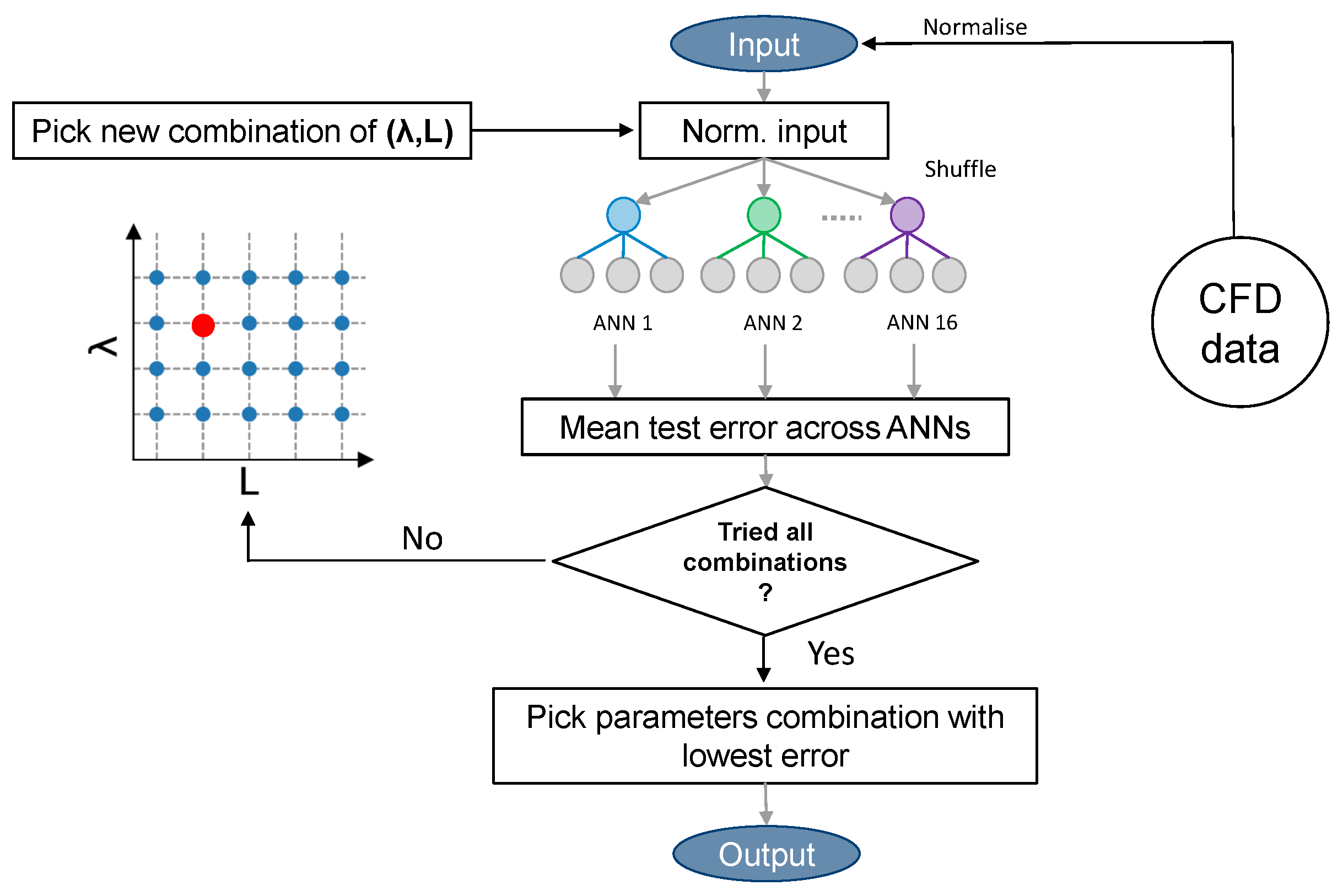
The weights determined in the optimisation process are influenced by multiple parameters, the hyperparameters, namely number of layers L and number of neurons per layer N L , training database size and regularisation factor λ . A baseline ANN with L = 2 , N L = 12 and λ = 10 4 will be used for the hyperparameters study. First, a training database independence study is carried out, using 5 different combinations of databases summarised in Table 2. The training/test split is kept constant at 80/20 for all the combinations. The gradient-based optimisation can lead to local minima of the cost function; therefore, 16 networks with different initial conditions and randomly reshuffled datasets are trained in parallel.
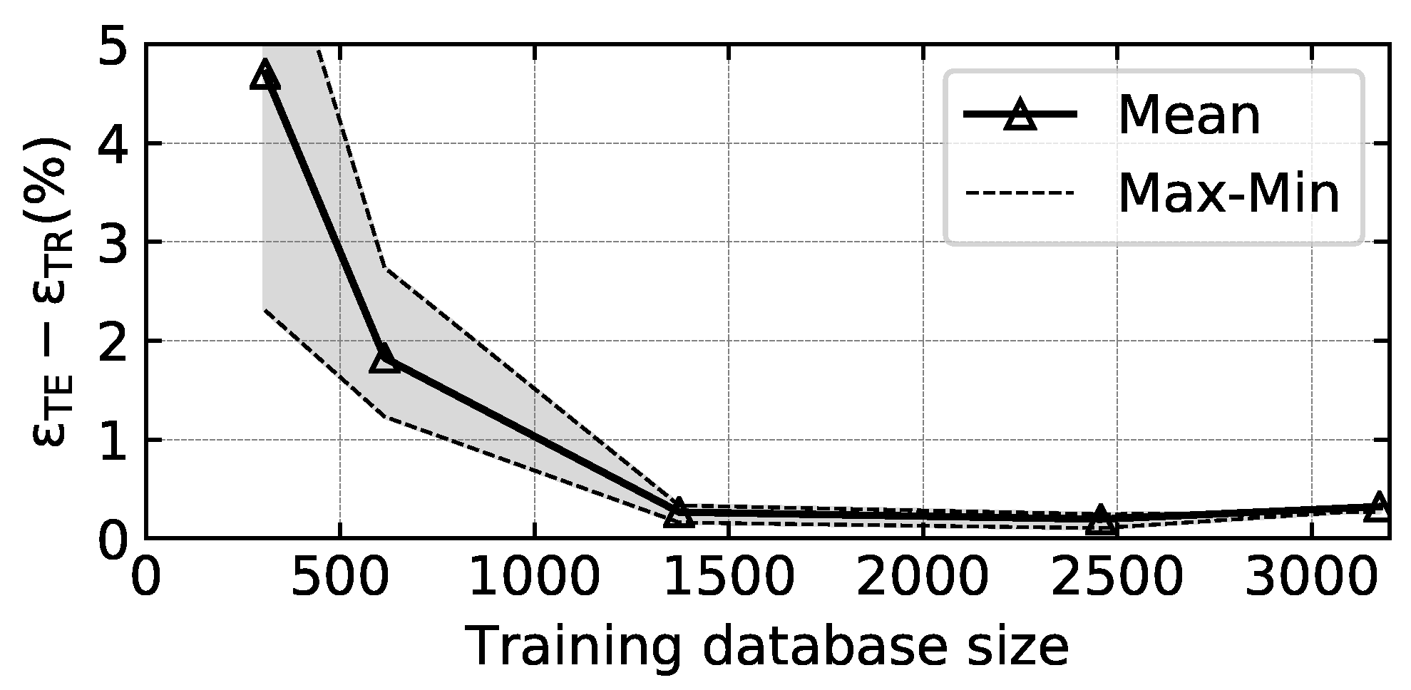
The difference between test and training error ( ε T E , ε T R ) is plotted in Figure 3. As the training database size increases, the difference between the test and training errors reduces to nearly zero, and thus, the accuracy of the ANN becomes independent of the training database size. Moreover the max-min envelope in Figure 3 converges to the mean value when all the datasets are used, indicating independence from initial conditions. The rest of the hyperparametric study is carried out using all data, with the training/test split discussed above.
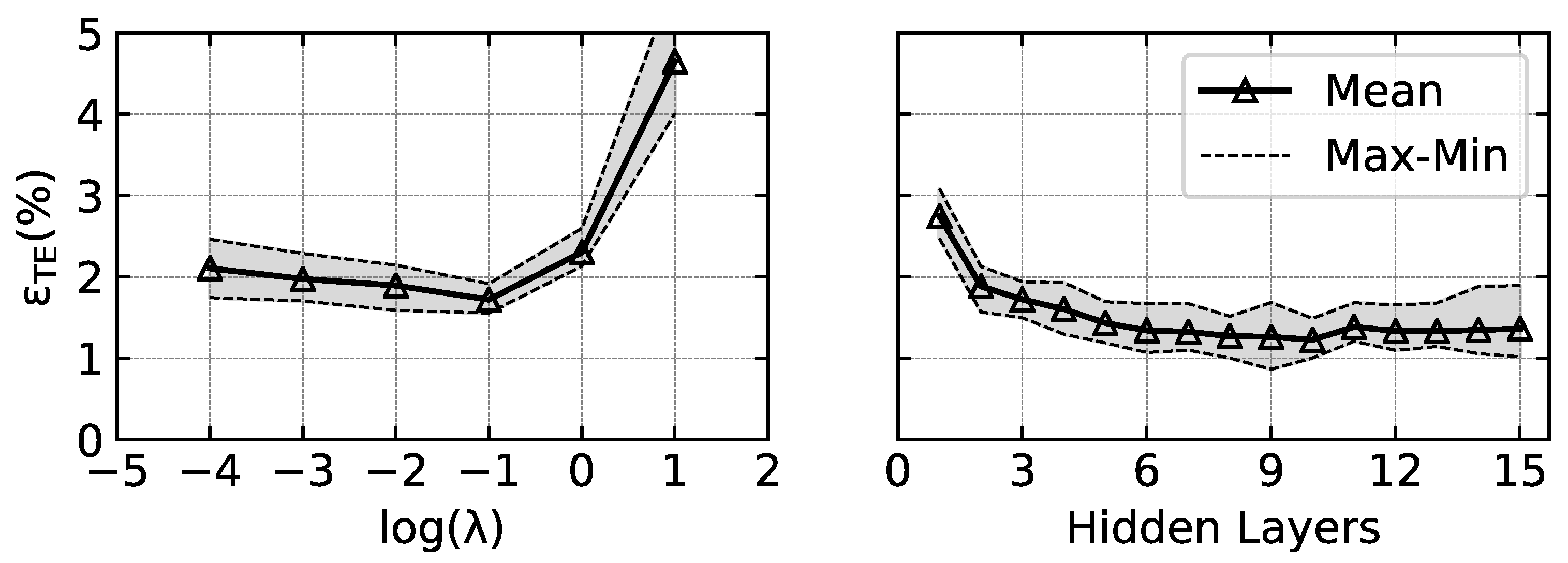
The hyperparameters are changed one at a time while keeping the others constant with the baseline setting; the number of neurons per layer, N L , is kept constant at a value of 12 throughout the study. The most appropriate value of λ depends on the number of layers in the ANN; in Figure 4 it is shown that the minimum error is achieved with λ = 10 1 when L = 2 . As L increases, so does the cost associated with the ANN weights (see Equation (9)); therefore, it is inferred that with L > 2 , the regularisation factor has to be λ 10 1 . In order to find the best combination of the two hyperparameters, the study of number of layers L is repeated 4 times, with λ = 10 1 , 10 2 , 10 3 , 10 4 , respectively. This approach is known as “grid search” and it is described in the flowchart in Figure 5.
It is observed that the minimum mean error value ( ε T E 1 % ) is achieved with λ = 10 4 and L = 10 . The ANN employed in the rest of this work is, therefore, characterised by the following hyperparameters: N L = 12 , L = 10 , λ = 10 4 .
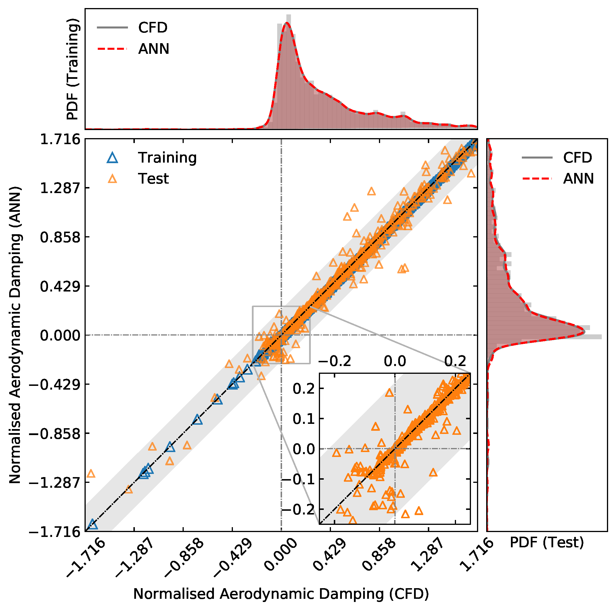
Figure 6 shows a good agreement between the PDFs of CFD and ANN predictions; almost none of the test data lie outside the 5 % confidence band (in grey).

3. Results

3.1. Validation

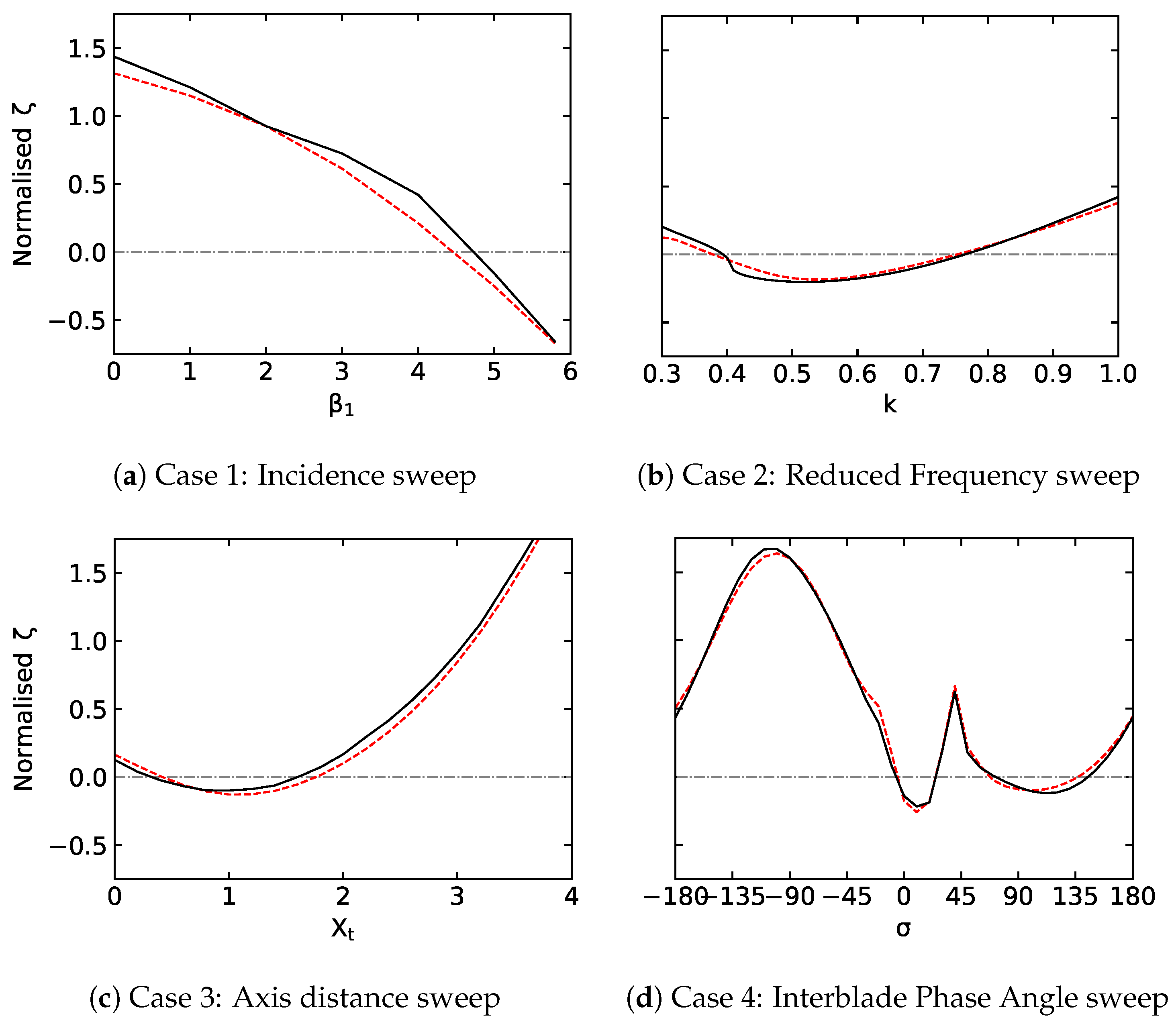
The following results show a comparison between ANN and CFD predictions. Four cases are setup to demonstrate the capability of the ANN: 4 out of 5 input variables are fixed while the remaining one is swept. The CFD computations employed in this comparison do not explicitly coincide with any training sample, they will therefore represent a further, and final, test to evaluate the machine-learnt surrogate model. The combination of parameters for the four comparisons are reported in Table 3. The results in Figure 7 show good agreement between ANN and CFD.
Figure 7a shows that for a blade vibrating in flap mode, in transonic flow, aerodynamic damping decreases with increasing flow incidence. The flow conditions for this case are very similar to what a fan blade section would experience as it moves up a constant speed characteristic. This behaviour has been already reported in the literature [8]. The ANN is able to follow the trend of the CFD closely, and to predict the flutter boundary within 0 . 2 , confirming that its predictions can be trusted for engineering-relevant cases. Figure 7b shows a reduced frequency sweep; at these flow conditions and with the given σ , the upstream and downstream cut-off frequencies are 0.230 and 0.408 , respectively. As the frequency of vibration is increased, the unsteady pressure fields upstream and downstream of the blade change from cut-on to cut-off. The frequencies at which this change takes place are the cut-off frequencies and their crossing is associated with a strong change in aerodynamic damping. The crossing in Figure 7b takes place at k = 0.408 and is visible by the drop in aerodynamic damping. The surrogate model captures the overall trend as well as the crossing of the zero damping line with good accuracy. Figure 7c shows a sweep of X t ; as the modeshape approaches a pure bending (increasing X t ), the aerodynamic damping increases, in agreement with the literature. The ANN is, again, able to follow the CFD closely. The peak in aerodynamic damping in Figure 7d is well predicted, both in location ( σ 40 ) and magnitude, and so is the overall shape of the curve.
The results discussed above show that the ANN is able to correctly predict aerodynamic damping across a range of flow conditions and structural parameters. Moreover, the surrogate model captures the zero damping crossing point (flutter boundary) with good accuracy. In the next subsection, an example of how the method can be used in a design environment is given.

3.2. Application

In this section, the application of this method to a hypothetical engineering problem is addressed. During the early design stage of a turbomachinery blade, the surrogate model predicts flutter for an aerodynamically optimised blade at some operating conditions. Even at the cost of reducing aerodynamic performance, the design parameters need to be adjusted to increase damping and regain stability. Under the assumption that a mechanical solution (e.g., introduction of under-platform dampers) is either not convenient or not possible at all (e.g., the blade is part of a blisk), the most viable solution is to increase aerodynamic damping. Traditional wisdom suggests that, for example, increasing reduced frequency is beneficial for aeroelastic stability. However, this generalisation has been shown to achieve mixed results in real applications (see Figure 7b). Therefore, there is a need for tools which can provide guidelines for blade re-design or optimisation to improve aerodynamic damping. This is the problem that the present method tries to tackle.
Take a blade behaving like Figure 7d as test case. Two intervals of σ are affected by flutter: 0 to 30 and 60 to 140 . The objective is to adjust the design parameters so that instability can be avoided. In order to achieve this goal, one can compute the normalised gradients (Equation (3)), and use them as a guide for deciding the best action to take in order to increase damping in an unstable configuration.
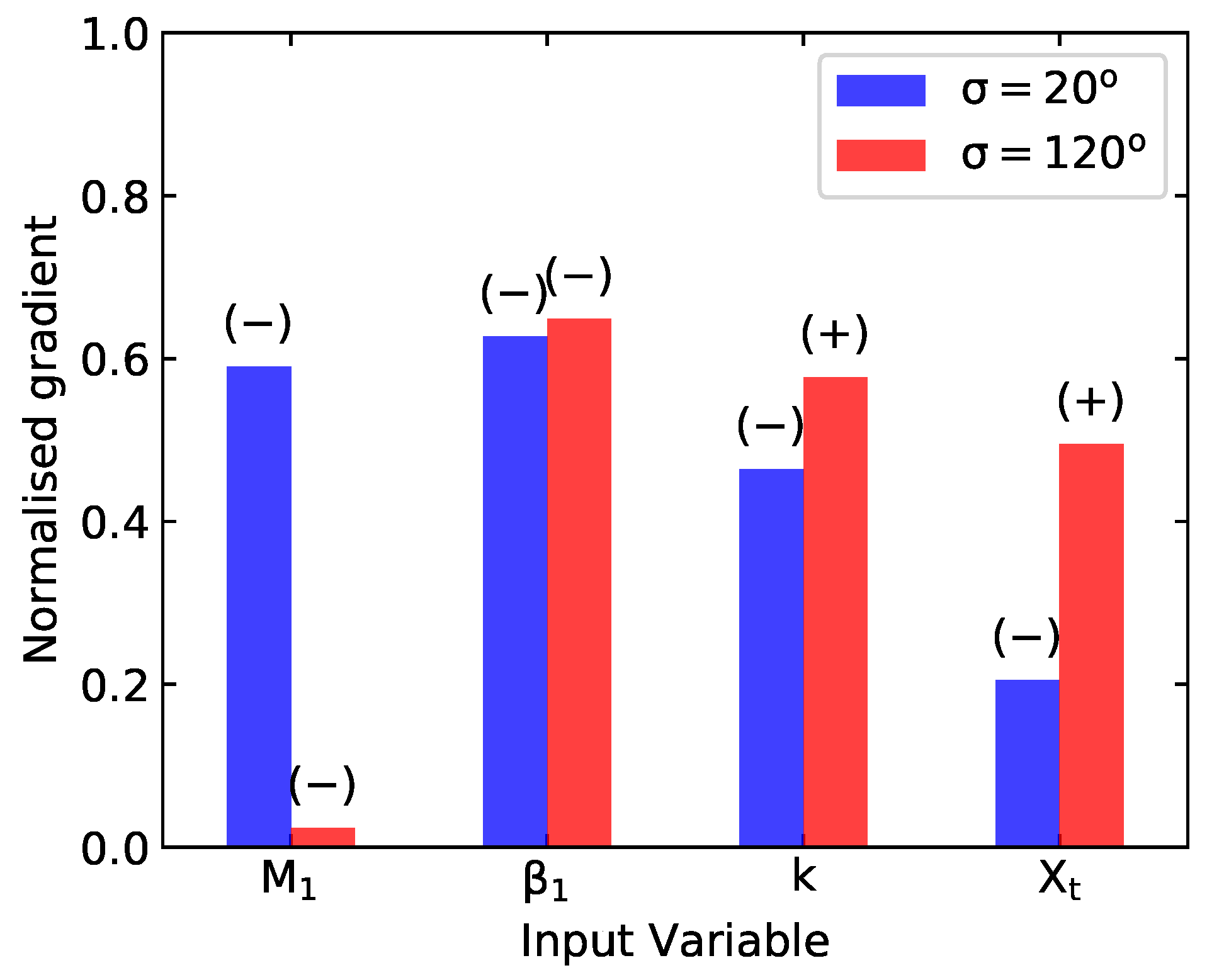
The normalised gradients at σ = 20 and σ = 120 are shown in Figure 8. The bar height, value of normalised gradient, is a measure of aerodynamic damping sensitivity, while the sign on top gives the type of correlation between input and output, i.e., a (+) sign indicates that an increase in input variable results in greater aerodynamic damping. The most important parameter in both cases of Figure 8 is β 1 which is negatively correlated with damping. M 1 is important for σ = 20 but exerts negligible influence at σ = 120 . The influence of k diminishes from σ = 120 to σ = 20 , and, most importantly, the nature of its correlation with aerodynamic damping is opposite between the two cases; i.e., an increment in k is beneficial at σ = 120 but detrimental at σ = 20 . Finally, X t shows the same behaviour as k. The previous considerations lead to the conclusion that, varying only one parameter, the most effective action one can take (for both Interblade Phase Angles) is to reduce the incidence of incoming flow onto the blade (e.g., restaggering the blade).
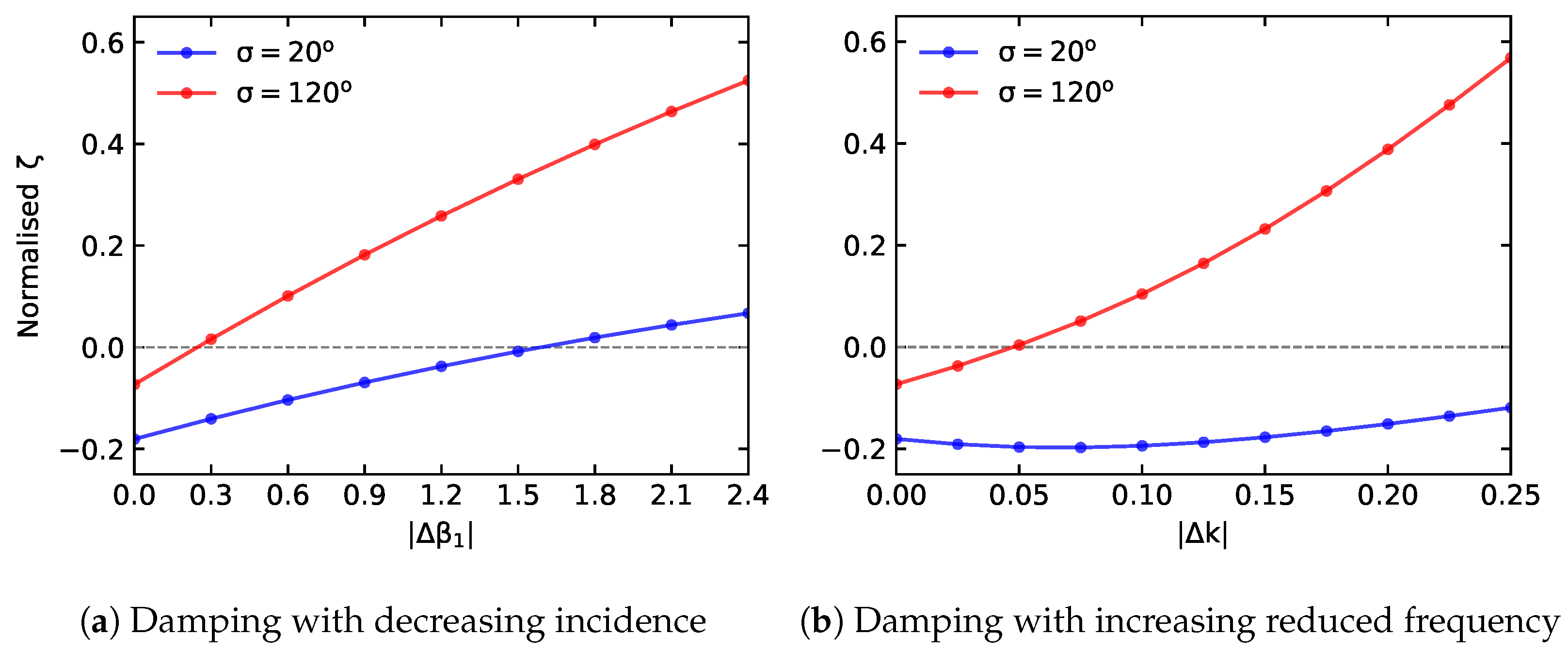
The change in aerodynamic damping due to variation in incidence angle and reduced frequency is shown in Figure 9. The predictions are results from the surrogate model. As expected, a reduction in incidence angle is beneficial for both Interblade Phase Angles (Figure 9a). In particular, a decrease of 0 . 3 is sufficient to stabilise σ = 120 , whereas a reduction of 1 . 8 is necessary to stabilise σ = 20 . Figure 9b confirms the contradicting behaviour of aerodynamic damping with respect to reduced frequency, for the two cases: an increase in k leads to a more stable blade at σ = 120 , but aggravates the instability at σ = 20 in the vicinity of the design point. The method also provides an “exchange rate” between different parameters so that the designer can make the best choice for improving flutter margin. For example, in Figure 9 for σ = 120 , a decrease of 0 . 3 in incidence is equivalent to an increase of, roughly, 0.06 in reduced frequency for eradicating flutter.
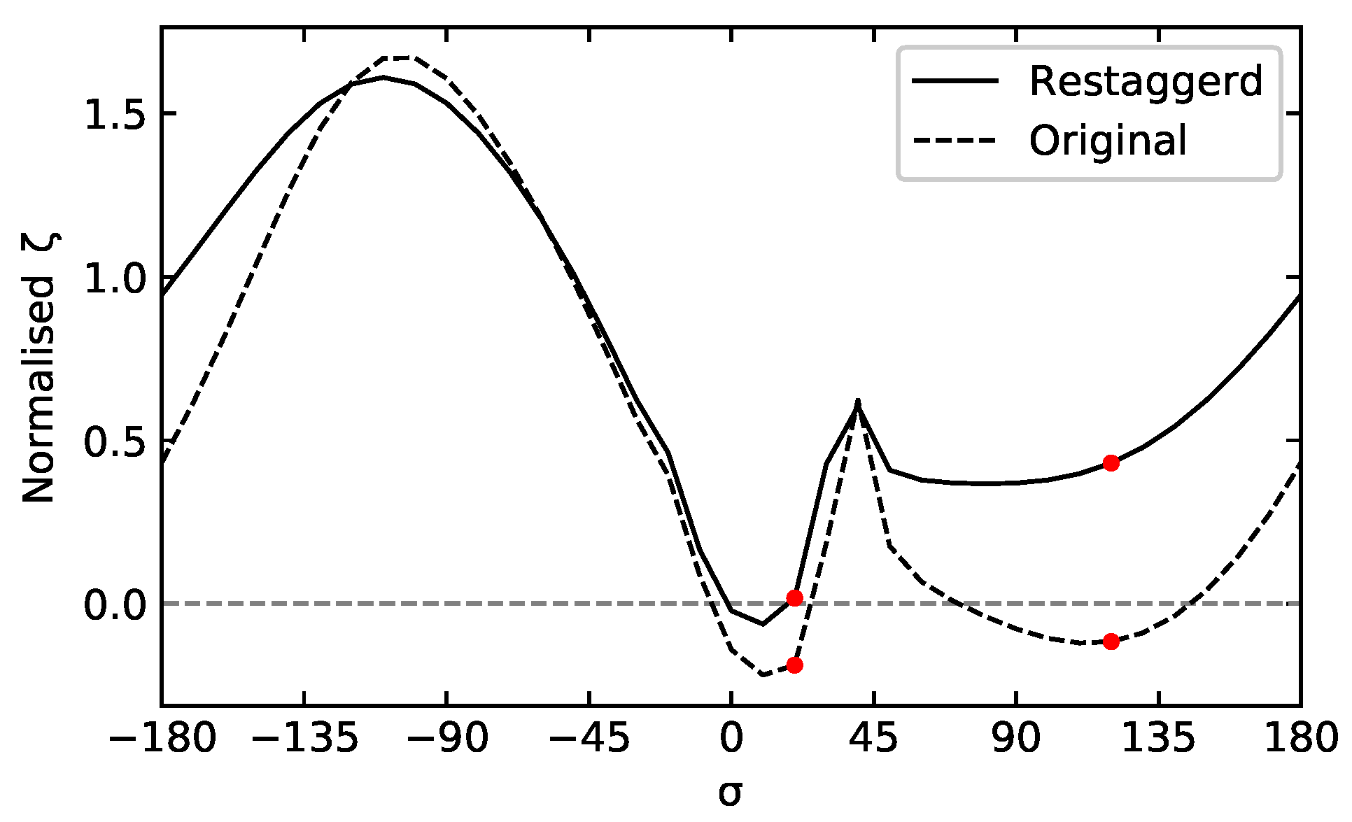
In summary, the surrogate model predicts that a decrease of 1 . 8 in flow incidence should stabilise the blade at both σ = 20 and σ = 120 . To verify this claim, a “restaggered” case is setup, where the inflow angle is kept constant and the incidence is reduced by restaggering the blade by 1 . 8 . The other parameters are kept constant. The aerodynamic damping predicted by the CFD is shown in Figure 10. As anticipated by the surrogate model, σ = 120 becomes highly stable while the point at σ = 20 sits just above the zero damping line. Two unstable points at σ = 0 and σ = 10 are still present: the process described above can be repeated for them and appropriate changes to the input variables can be made to induce stability at these Interblade Phase Angles.

4. Conclusions and Future Work

A machine-learning-based sensitivity analysis has been presented. The surrogate model has been trained on results from a linearised aeroelastic solver and its validity has been tested through evaluation of relative errors. The results concern a flap modeshape, with different Interblade Phase Angles, across a range of reduced frequencies, flow conditions and consequent acoustic waves regimes. It has been shown that the sensitivity analysis can be used as a guide to take appropriate measures to stabilise two unstable operating points; therefore, constituting a redesign tool for the given airfoil geometry. This preliminary study shows how summary measures of influence of design parameters can be easily extracted and presented with data-driven approaches, such as machine learning, rather than classical methods of investigation. The results in this work are obtained with a simple artificial neural network which makes no assumption regarding the flow physics of turbomachinery. Furthermore, the results are only valid for the airfoil geometry used in the training phase. Future work will focus on addressing these limitations by embedding known physics into the cost function (e.g., continuity), and by training the model on physically relevant steady state features (e.g., shock strength), independent of geometry.
Author Contributions

Conceptualization, M.R., M.V. and F.Z.; methodology, M.R., M.V., F.Z.; software, M.R.; formal analysis, M.R.; investigation, M.R., M.V., F.Z.; data curation, M.R.; writing—original draft preparation, M.R.; writing—review and editing, M.R., M.V. and F.Z.; visualization, M.R.; supervision, M.V. and F.Z.; funding acquisition, M.V. All authors have read and agreed to the published version of the manuscript.

Funding

This research received no external funding.

Institutional Review Board Statement

Not applicable.

Informed Consent Statement

Not applicable.

Data Availability Statement

Not applicable.

Acknowledgments

The authors would like to thank Paul Petrie-Repar from RPMTurbo for providing the aeroelastic solver used in this work.

Conflicts of Interest

The authors declare no conflict of interest.

Abbreviations

The following abbreviations are used in this manuscript:
ANNArtificial Neural Network
CFDComputational Fluid Dynamics
MUSCLMonotonic Upstream-Centered Scheme for Conservation Laws
URANSUnsteady Reynolds-averaged Navier–Stokes
PDFProbability Density Function
GMRESGeneralized Minimal Residual Method

Appendix A. Computational Cost

The steady state solver uses a pseudo-time stepping technique to bring the solution to convergence. In this study, a steady CFD solution is considered converged if every point in the domain has a density residual of order 10 6 . On average, the equivalent CPU time elapsed to obtain a converged solution for this case is 8400 s.
The unsteady solver uses a preconditioned GMRES scheme to find the solution to the system arising from the linearisation of the URANS equations. In this study, an unsteady CFD solution is considered converged if the residual is of order 10 6 . On average, the equivalent CPU time elapsed to obtain a converged solution for this case is 20 s.
In total, the creation of the 5 databases employed in this study took an estimated 9280 CPU hours.
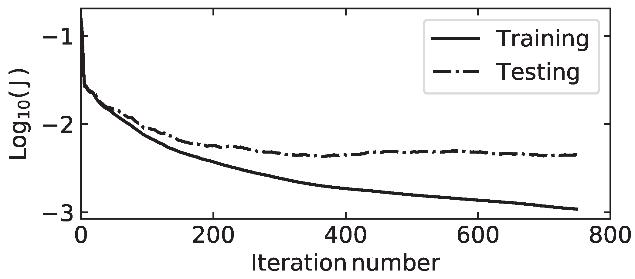
The ANN employed in this study runs on CPU and the optimisation process performs a fixed number of steps, 750. The number of iterations was chosen so that the different ANNs would not suffer from excessive underfitting or overfitting, so called “early stopping” regularization. The cost function convergence history for the ANN employed in this work is shown in Figure A1.
Figure A1. Plot of cost function convergence.
Ijtpp 06 00039 g0a1
A total of 1072 different ANNs have been trained to find the best combination of parameters, yielding an estimated 194 equivalent CPU hours. The results in Figure 7 consist of 8 steady and 135 unsteady simulations. The predictions from the CFD have been obtained in an estimated 19 equivalent CPU hours, whereas the ANN produced its results in 4.6 CPU milliseconds.

References

  1. AGARD. Manual on Aeroelasticity in Axial-Flow Turbomachines; AGARD-AG-298; North Atlantic Treaty Organization: Neuilly sur Seine, France, 1987. [Google Scholar]
  2. Chi, R.M.; Srinivasan, A.V. Some Recent Advances in the Understanding and Prediction of Turbomachine Subsonic Stall Flutter. J. Eng. Gas Turbines Power 1985, 107, 408–417. [Google Scholar] [CrossRef]
  3. Crawley, E.F.; Ducharme, E.H. Parametric Trends in the Flutter of Advanced Turboprops. J. Turbomach. 1990, 112, 741–750. [Google Scholar] [CrossRef]
  4. Srinivasan, A.V. Flutter and Resonant Vibration Characteristics of Engine Blades. J. Eng. Gas Turbines Power 1997, 119, 742–775. [Google Scholar] [CrossRef]
  5. Whitehead, D.S. Vibration and Sound Generation in a Cascade of Flat Plates in Subsonic Flow. 1972. Available online: https://reports.aerade.cranfield.ac.uk/bitstream/handle/1826.2/2959/arc-rm-3685.pdf?sequence=1&isAllowed=y (accessed on 31 January 2020).
  6. Akai, T.J.; Atassi, H. Aerodynamic and Aeroelastic Characteristics of Oscillating Loaded Cascades at Low Mach Number-Part II: Stability and Flutter Boundaries. J. Eng. Power 1980, 102, 352–356. [Google Scholar] [CrossRef]
  7. Atassi, H.; Akai, T.J. Aerodynamic and Aeroelastic Characteristics of Oscillating Loaded Cascades at Low Mach Number-Part 1: Pressure Distribution, Forces, and Moments. J. Eng. Power 1980, 102, 344–351. [Google Scholar] [CrossRef]
  8. Vahdati, M.; Cumpsty, N. Aeroelastic Instability in Transonic Fans. ASME J. Eng. Gas Turbines Power 2016, 138, 022604. [Google Scholar] [CrossRef]
  9. Tyler, J.M.; Sofrin, T.G. Axial Flow Compressor Noise Studies; SAE Technical Pape; SAE International: Warrendale, PA, USA, 1962. [Google Scholar] [CrossRef]
  10. Panovsky, J.; Kielb, R.E. A Design Method to Prevent Low Pressure Turbine Blade Flutter. J. Eng. Gas Turbines Power 1999, 122, 89–98. [Google Scholar] [CrossRef]
  11. Lee, K.B.; Wilson, M.; Vahdati, M. Numerical Study on Aeroelastic Instability for a Low Speed Fan. J. Turbomach. 2016, 139, 071004. [Google Scholar] [CrossRef]
  12. Dowell, E.H. (Ed.) A Modern Course in Aeroelasticity; Springer: Berlin/Heidelberg, Germany, 2015; pp. 428–429. [Google Scholar]
  13. Isomura, K.; Giles, M.B. A Numerical Study of Flutter in a Transonic Fan. J. Turbomach. 1998, 120, 500–507. [Google Scholar] [CrossRef]
  14. He, X.; Zhao, F.; Vahdati, M. Uncertainty Quantification of Spalart-Allmaras Turbulence Model Coefficients for Simplified Compressor Flow Features. J. Fluids Eng. 2020, 142, 091501. [Google Scholar] [CrossRef]
  15. Duraisamy, K.; Iaccarino, G.; Xiao, H. Turbulence Modeling in the Age of Data. Annu. Rev. Fluid Mech. 2019, 51, 357–377. [Google Scholar] [CrossRef] [Green Version]
  16. Xiao, H.; Cinnella, P. Quantification of model uncertainty in RANS simulations: A review. Prog. Aerosp. Sci. 2019, 108, 1–31. [Google Scholar] [CrossRef] [Green Version]
  17. Stapelfeldt, S.; Vahdati, M. On the Importance of Engine-Representative Models for Fan Flutter Predictions. J. Turbomach. 2018, 140, 081005. [Google Scholar] [CrossRef]
  18. Frannson, T.; Verdon, J. Update Report on Standard Configurations for Unsteady Flow through Vibrating Axial-flow Turbomachine Cascades. Rep. R. Inst. Technol. Stock. Swed. 1991. Available online: https://www.rpmturbo.com/testcases/STCF/STCF1to10/Documents/SC2110.92update.pdf (accessed on 31 March 2020).
  19. Petrie-Repar, P.J.; McGhee, A.; Jacobs, P.A.; Gollan, R. Analytical Maps of Aerodynamic Damping as a Function of Operating Condition for a Compressor Profile. In Proceedings of the Turbo Expo: Power for Land, Sea, and Air, Barcelona, Spain, 8–11 May 2006; Volume 5, pp. 1133–1144. [Google Scholar]
  20. Frey, C.; Ashcroft, G.; Kersken, H.P.; Schlüß, D. Flutter Analysis of a Transonic Steam Turbine Blade with Frequency and Time-Domain Solvers. Int. J. Turbomach. Propuls. Power 2019, 4, 15. [Google Scholar] [CrossRef] [Green Version]
  21. Rendu, Q.; Vahdati, M.; Salles, L. Radial Decomposition of Blade Vibration to Identify a Stall Flutter Source in a Transonic Fan. J. Turbomach. 2019, 141, 101011. [Google Scholar] [CrossRef]
  22. Zhao, F.; Nipkau, J.; Vahdati, M. Influence of acoustic reflections on flutter stability of an embedded blade row. Proc. Inst. Mech. Eng. Part A J. Power Energy 2016, 230, 29–43. [Google Scholar] [CrossRef]
  23. McKay, M.D.; Beckman, R.J.; Conover, W.J. A Comparison of Three Methods for Selecting Values of Input Variables in the Analysis of Output from a Computer Code. Technometrics 1979, 21, 239–245. [Google Scholar]
  24. Lecun, Y. Generalization and network design strategies. In Connectionism in Perspective; Pfeifer, R., Schreter, Z., Fogelman, F., Steels, L., Eds.; Elsevier: Amsterdam, The Netherlands, 1989. [Google Scholar]
  25. Fletcher, R. Practical Methods of Optimization; Number v. 2 in A Wiley-Interscience Publication; Wiley: Hoboken, NJ, USA, 1987. [Google Scholar]
Figure 1. Example of steady state solution.
Ijtpp 06 00039 g001
Figure 2. Schematic illustration of modeshape at different X t .
Ijtpp 06 00039 g002
Figure 3. Training database independence study.
Ijtpp 06 00039 g003
Figure 4. Hyperparameters study.
Ijtpp 06 00039 g004
Figure 5. Flowchart for hyperparameters selection.
Ijtpp 06 00039 g005
Figure 6. PDF and scatter plot of CFD data points and ANN “reproductions”.
Ijtpp 06 00039 g006
Figure 7. Comparison of ANN (dashed red line) and CFD (solid black line) predictions.
Ijtpp 06 00039 g007
Figure 8. Normalised gradients for Case 4 at σ = 20 and σ = 120 .
Ijtpp 06 00039 g008
Figure 9. Change in normalised damping at σ = 20 and σ = 120 .
Ijtpp 06 00039 g009
Figure 10. CFD prediction of normalised damping for “restaggered” blade.
Ijtpp 06 00039 g010
Table 1. Intervals of design parameters.
Parameter MinMax
M 1 Inlet Mach Number 0.5 0.9
β 1 Incidence (difference with nominal) 0 + 6
kReduced Frequency 0.4 1.5
X t Non dimensional Twist Axis distance 0.0 4.0
σ Interblade Phase Angle 180 180
Table 2. Data for training database independence study.
DataTotal SizeTraining DataTest DataTrained ANNs
db 1 db 2 384 80 % 20 % 16
db 2 db 3 768 80 % 20 % 16
db 3 db 4 1536 80 % 20 % 16
db 4 db 5 3072 80 % 20 % 16
All dbs3967 80 % 20 % 16
Table 3. Input parameters for ANN sweep test.
M 1 β 1 k X t σ
Case 1 0.8 Sweep 0.5 3.0 20
Case 2 0.55 + 5 Sweep 1.5 20
Case 3 0.7 + 6 0.7 Sweep 0
Case 4 0.55 + 5 0.5 1.0 Sweep
Publisher’s Note: MDPI stays neutral with regard to jurisdictional claims in published maps and institutional affiliations.