Unsteady Simulation of a Transonic Turbine Stage with Focus on Turbulence Prediction

Abstract

The flow in a transonic turbine stage still poses a high challenge for the correct prediction of turbulence using an eddy viscosity model. Therefore, an unsteady RANS simulation with the k-ω SST model, based on a preceding study of turbulence inlet conditions, was performed to see if this can improve the quality of the flow and turbulence prediction of an experimentally investigated turbine flow. Unsteady Q3D results showed that none of the different turbulence boundary conditions could predict the free-stream turbulence level and the maximum values correctly. Luckily, the influence of the boundary conditions on the velocity field proved to be small. The qualitative prediction of the complex secondary flows is good, but there is lacking agreement in the prediction of turbulence generation and destruction.

1. Introduction

Although CFD codes are already highly developed and able to predict the flow even through very complex geometries, still assumptions and simplifications are necessary concerning turbulence. The correct prediction of turbulence in a highly loaded turbine stage using a RANS approach still poses a challenge. Therefore, experiments in test rigs at realistic flow conditions where turbulence data are also acquired support the development and evaluation of CFD codes.

Therefore, at Graz University of Technology, Göttlich et al. [1] performed Laser Doppler Velocimetry (LDV) in a transonic turbine stage, where they measured the unsteady velocity and turbulence in planes after the stator and rotor. Based on the experimental data, Pieringer et al. [2] studied the secondary flow effects and the interaction of the rotor tip leakage vortex with the main flow with a steady CFD simulation. Since the agreement with the measurements was not completely satisfying, the fillets of the nozzle blades were additionally modelled, but the agreement with the measurements did not improve [3].

In a new attempt, Pecnik et al. [4] applied different turbulence models in the steady simulation of the transonic stage, where the k-ω SST model by Menter [5] could best predict the flow separation at the trailing edge of the stator blade, but deviations to the measurement data still remained. Therefore, in this work, based on [6], a further attempt with an unsteady simulation of the transonic stage flow using the k-ω SST model is presented where particular attention was paid to the comparison of the measured turbulence after the rotor with the predicted one. This shall help to clarify the limitations of RANS simulations in predicting turbulence in highly loaded transonic turbine stages.

2. Test Facility and Experimental Data

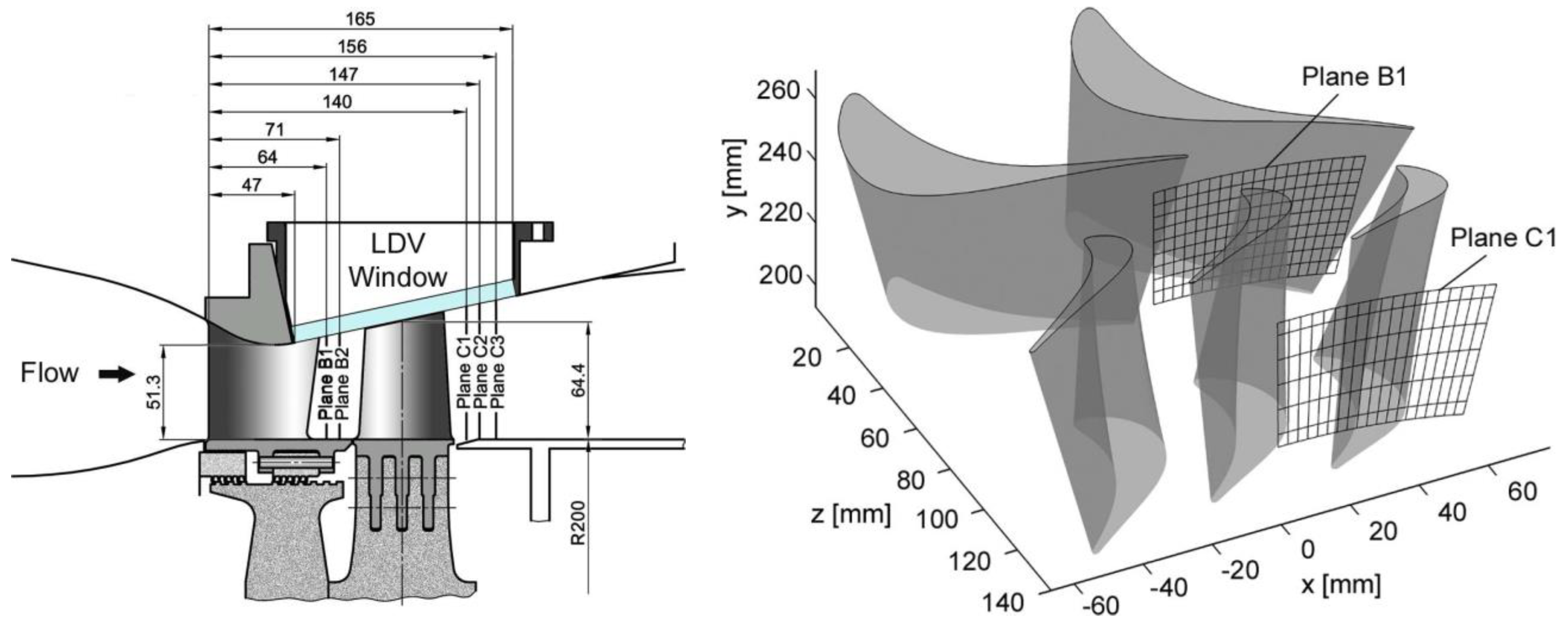
The Institute for Thermal Turbomachinery and Machine Dynamics at Graz University of Technology has been operating a transonic test turbine as a cold-flow, open-circuit facility since 2001. The first test object was a transonic turbine stage where laser Doppler velocimetry (LDV) was used to measure the unsteady flow [1]. Figure 1 (left) shows the meridional flow contour with stator and rotor blade and the main dimensions. The convergent–divergent flow path accelerates the flow to supersonic velocities. Stagnation values of pressure and temperature were measured with probes 66 mm in front of the stator leading edge and the outlet static pressure was measured in a plane 158 mm downstream of the stator leading edge. Geometrical data of the blades and important operating conditions are summarized in

Table 1. Stage geometrical data and operating conditions.

Number of nozzle guide vanes	24
Number of rotor blades	36
Nozzle chord (mid-span) [mm]	78.9
Nozzle turning angle [deg.]	70
Rotor blade chord (mid-span) [mm]	55.9
Rotor blade turning angle [deg.]	107
Nozzle height at exit [mm]	55.1
Rotor blade height at exit [mm]	69.2
Tip clearance/blade height [%]	1.4
Pressure ratio ptot,in/pout	3.50
Reynolds number nozzle exit	2.57 × 106
Reynolds number rotor blade exit	1.69 × 106

. The profile geometry of the 24 stator blades and the 36 rotor blades is indicated in Figure 1 (right). These blade numbers implicate a circumferential periodicity of 30 deg.

In the outer casing a glass window was mounted to allow LDV access to the flow channel. LDV data were collected in plane B1 after the stator and plane C1 after the rotor (see Figure 1). The measurement domain covered 15 deg. circumferential spacing (=1 stator pitch), so that by correct phase shifting the full periodic domain of 30 deg. corresponding to 2 stator and 3 rotor channels could be obtained. Due to reflections at the hub and the glass window, the measurements covered approximately 25% to 88% relative span in B1 and 25% to 80% relative span in C1 (see Figure 1, right). Nine radial lines in plane B1 and seven radial lines in plane C1 were traversed with 20 measurement positions per line, where approximately 80,000 velocity bursts were collected. They were assigned to the proper rotor position, i.e., 40 different stator-rotor positions per rotor blade pitch (=10 deg.), with the help of a trigger signal provided by the shaft monitoring system.

In order to get the turbulence locally and over time by the variance, the instantaneous velocity vector $v_i$ of each burst was decomposed as follows

$$v_i=\overline{v}+v^{\prime }=\stackrel{=}{v}+\tilde{v}+v^{\prime }$$

(1)

where $\overline{v}$ is the ensemble-averaged velocity, $\stackrel{=}{v}$ is the time-averaged velocity, $\tilde{v}$ is the periodic velocity component, and $v^{\prime }$ is the unresolved velocity component, i.e., the turbulent fluctuation. With 40 evaluation windows, the number of velocity samples per window was still high enough to allow the determination of mean value and level of turbulence at reasonable uncertainty. For a confidence level of 95%, an uncertainty of 3.5 m/s in and 0.9 m/s outside the rotor wake for the ensemble-averaged velocity as well as 11 m/s in and 2.5 m/s outside the rotor wake for the unresolved velocity were found.

Since a two-dimensional LDV system was applied, only the velocities in the axial and circumferential direction were measured. Therefore, for the calculation of the turbulence kinetic energy k reliable estimations on the fluctuations in radial direction were needed. For this, turbulence measurements with a CTA system, performed by Bauinger et al. [7] inside a two-stage configuration in our test rig, were analyzed and the ratio of the radial fluctuations to the mean of the axial and circumferential fluctuations was evaluated. In a plane after the turning strut of the turbine center frame, the average ratio was 1.08 with a standard deviation of 0.4. In a plane shortly after the LP blade, the average ratio was 0.77 with a standard deviation of 0.17. Based on this ratio, the turbulence kinetic energy k can be estimated as

$$k=\left(0.69÷ 0.77\right)(\overline{{u^{\prime }}^2}+\overline{{v^{\prime }}^2})$$

(2)

For the following comparisons with the measurement data, a ratio of 0.75 was used, which corresponds to the variance of the radial fluctuations as the mean of the variances in the two other directions. Compared to the lower value of 0.69, this means an overestimation of k by 8%.

Another uncertainty comes from the definition of the turbulence kinetic energy in the simulations based on a Favre- (mass-) averaging of velocity (see Equation (3)). A simple estimation of the error due to the different definitions showed only for the case of very high turbulence deviations of 2%, whereas it is mostly below 1% [6].

$$k_{Favre}=\frac{1}{2\overline{\rho }}(\overline{{{\rho u}^{″}}^2}+\overline{{{\rho v}^{″}}^2}+\overline{{{\rho w}^{″}}^2})$$

(3)

3. Numerical Setup

3.1. Flow Solver

The computations were performed with the Navier–Stokes code LINARS, developed at the Institute for Thermal Turbomachinery and Machine Dynamics (ITTM) by Pecnik et al. [4], which has been successfully utilized for the solution of numerous applications. The code solves the compressible Reynolds averaged Navier–Stokes equations in conservative form by means of a fully implicit, time-marching, finite-volume method. Structured grids are utilized in multi-block assignment. The code is parallelized based on the grid blocks.

The inviscid fluxes are discretized with the upwind flux difference splitting method by Roe. A higher order of spatial accuracy for the convective fluxes is achieved through a monotone upstream-centered scheme (MUSCL). A limiter is applied to avoid numerical instabilities. The viscid flux vector at the cell interfaces is constructed in a central-differencing manner using Green’s theorem. A linear set of algebraic equations is obtained by discretization in time with the Newton–Raphson procedure. For this investigation, turbulence was modelled with the k-ω SST turbulence model [5].

3.2. Computational Mesh

The block-structured computational mesh was generated with the in-house meshing tool AIGrid3D. In order to have full flow periodicity in the unsteady simulation, a 30-deg. segment comprising two stator blades and three rotor blades had to be modelled. Figure 2 (left) shows the resulting mesh, consisting of 57 blocks. Special care was laid on the mesh quality in the rotor tip leakage, as shown by the block structure in Figure 2 (right). The total number of cells was nearly 10 million. The y+ value of all wall cells was evaluated and showed a mean value of 0.8; 97% of all cells exhibited a value below 1.2. From preceding mesh studies on similar configurations, this mesh quality proved sufficient to obtain grid independent results (see, e.g., [8]).

3.3. Boundary Conditions and Solver Parameters

The boundary conditions are given in

Table 2. Boundary Conditions.

Rotational speed [rpm]	10,617
Inlet total pressure [Pa]	3.332 × 105
Inlet total temperature [K]	402.7
Inlet turbulence intensity [%]	12/18
Inlet turbulent length scale [mm]	1/5
Outlet static pressure at inner casing [Pa]	0.90 × 105

. Constant total pressure and total temperature as well as axial inflow were prescribed at the inlet boundary. At the beginning, a turbulence intensity of 12% and a mixing length of 1 mm was applied and later adapted based on the comparison with the measurements (see below). At the outlet, the static pressure was prescribed at the inner contour; radial equilibrium was applied. The rotational speed was 10,617 rpm.

For the unsteady simulation, a constant time-step corresponding to 1/40 deg. of rotor rotation was used, so that 1200 time iterations were necessary to cover one periodic segment of 30 deg. Periodic fluctuations were monitored and periodic convergence was achieved after 180 deg. of rotation. Data evaluation was done after one full rotation. Two Newton subiterations were used to improve the temporal accuracy. The computational time for one rotation was approx. 190 h, using 24 Intel(R) Xeon(R) X7560 8-core 2.26 GHz CPUs.

4. Results

4.1. Study of Inlet Turbulence

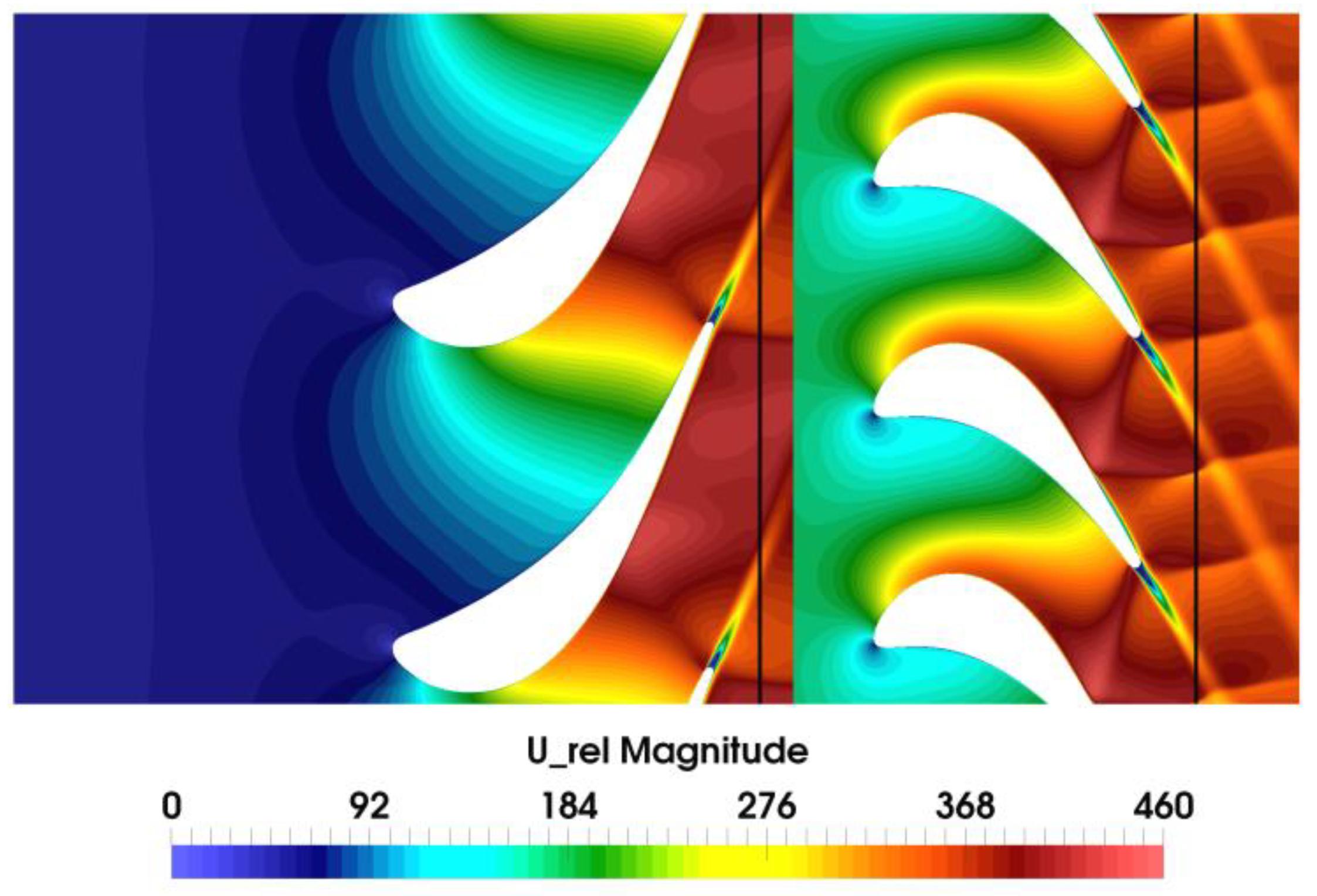
Figure 3 shows the absolute and relative velocity at mid-span from a 3D steady simulation illustrating the main flow features. In the stator as well as in the rotor, the flow was strongly accelerated, resulting in two shock systems emanating from the trailing edge. The pressure-side shock was reflected at the neighboring blade suction side. The stator flow remained supersonic to the rotor inlet. In the rotor, the reflected shock was still very strong and formed a parallel shock to the suction-side trailing-edge shock leaving the rotor.

In a steady simulation, at the mixing plane between stationary and rotating domain the turbulence kinetic energy was averaged, leading to an increase in the free-stream turbulence and an extinction of the wake turbulence. Therefore, an unsteady simulation needed to be performed in order to study turbulence generation and transport.

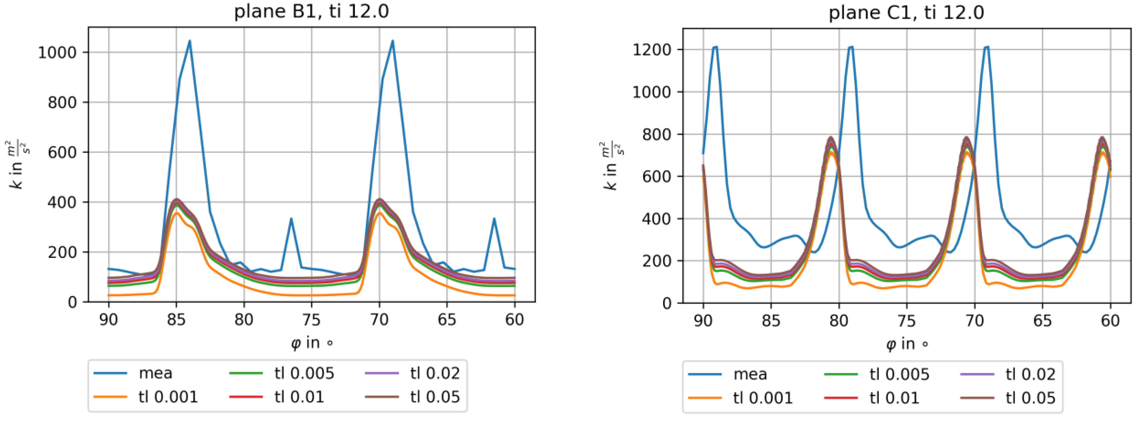
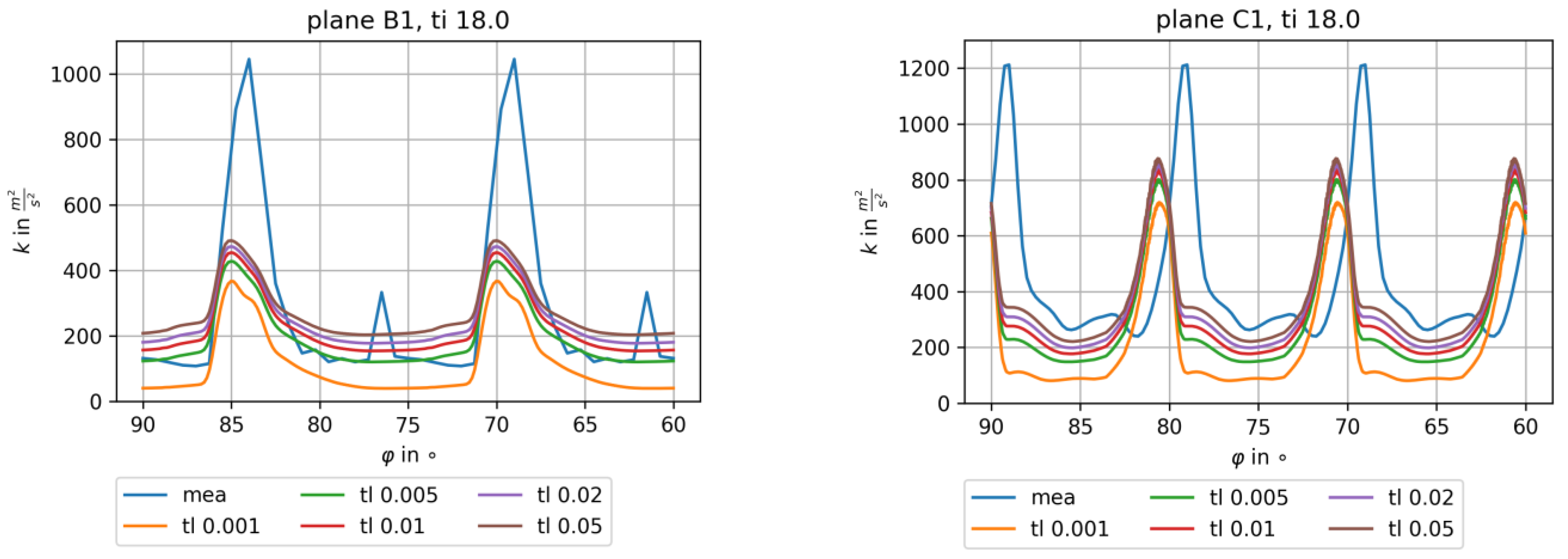
For the used test case, turbulence measurements in the inflow were not performed, but for other test configurations a very high turbulence intensity of 12–15% was found for the test rig. However, no data on the turbulent length scale were known. In order to find reasonable turbulence inlet boundary conditions, an unsteady Q3D flow study for varying turbulence inlet conditions was performed. The turbulence intensity was varied between 12% and 21% and the length scale between 1 mm and 50 mm. The results were compared with the measurements of the turbulence kinetic energy in planes B1 and C1, and are shown for a turbulence intensity of 12% and 18% in Figure 4 and Figure 5, respectively. The values were averaged over time and between the flow channels.

The measured maximum values in the wake of approx. 1000 m²/s² after the stator and 1200 m²/s² after the rotor could not be achieved by far by any inlet condition. Additionally, the small second peak in B1 and C1 in mid-channel was not found. There was also a clear shift in the circumferential position of the rotor wake, which was attributed to difficulties in determining the exact rotor position with the used trigger signal.

For a turbulence intensity of 12%, there was little influence of the chosen value of the turbulent length scale. In the free-stream, a slight underprediction occurred after the stator and a strong deviation after the rotor. For an inlet turbulence of 18%, the influence of the turbulent length scale was more pronounced. For a value of 5 mm, the free-stream level after the stator was well captured, whereas the rotor free-stream turbulence was again underpredicted for all values of the turbulent length scale. The turbulence level there depends strongly on the turbulent mixing process of the incoming stator flow, which was difficult to accurately predict with a linear eddy-viscosity model. On the other hand, the high values in the stator wakes were also not found in the simulation, so that these two effects can partly explain the discrepancy in the rotor free-stream turbulence. As a compromise between stator and rotor flow agreement, a turbulence intensity of 18% and a turbulent length scale of 5 mm were chosen for the succeeding unsteady, full 3D flow simulations.

4.2. Rotor Secondary Flow

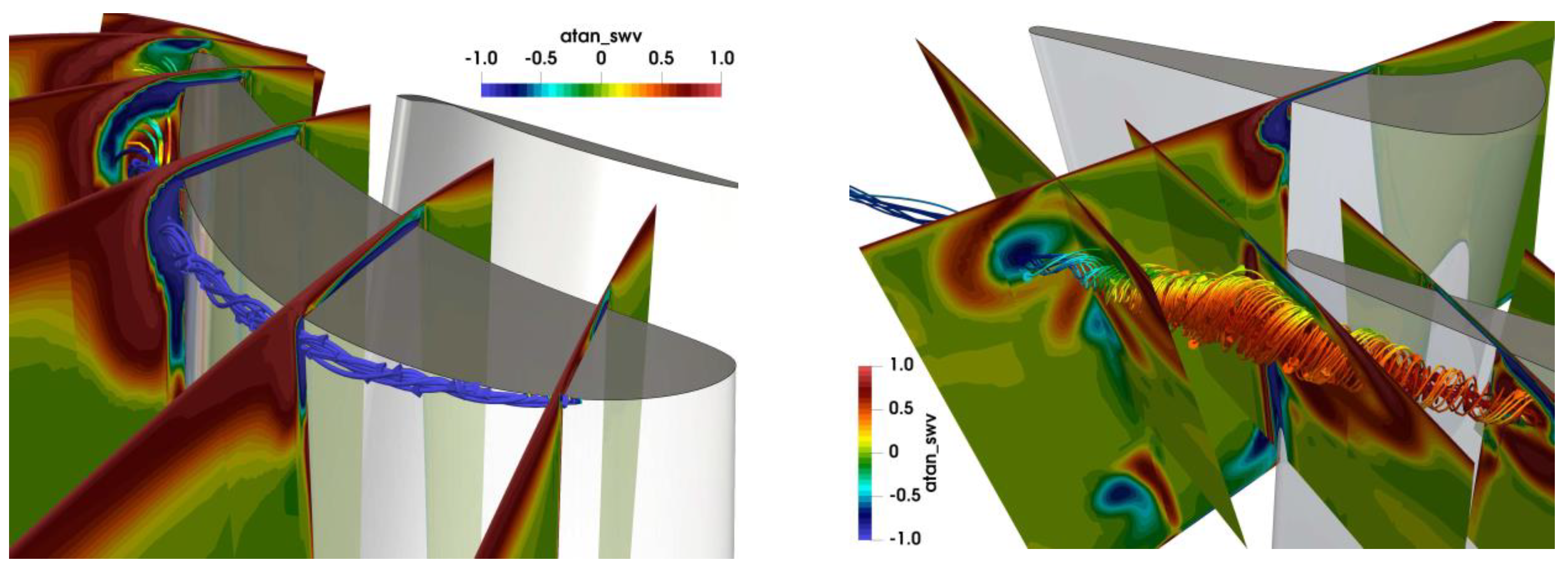
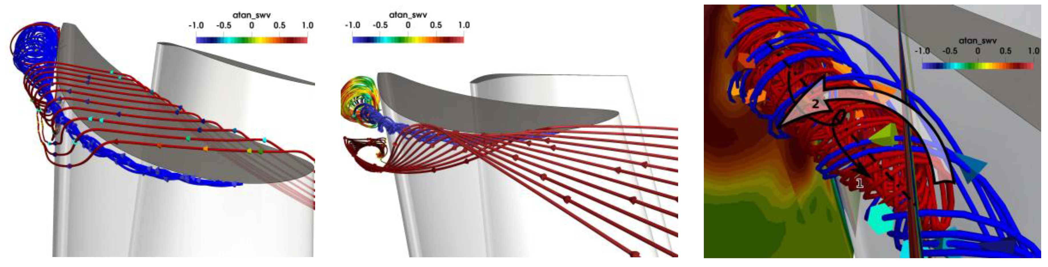
In order to better understand the turbulence generation and structures in the stage, at first the secondary flow in the rotor was presented. In Figure 6, contours of normalized streamwise vorticity (SWV) and streamlines colored by SWV explain the formation of the secondary flow in the hub region. Positive values of SWV indicate clockwise rotation. In the left figure, the streamlines originating from the horseshoe vortex at the leading edge are depicted. The pressure-side leg moved immediately towards the suction side of the neighboring blade and was pushed towards mid-span at the channel exit. It kept its strong counterclockwise sense of rotation. The suction-side leg kept its original sense of rotation only for a short term and then also switched to counterclockwise rotation. The right figure is a view from the bottom in span-wise direction. The large blue zone of counterclockwise rotation, where the pressure-side leg of the horse-shoe vortex ends, was caused by the lower channel vortex. The suction side-leg rotated slowly around the vortex core. A small zone of clockwise vorticity starting at mid-chord in the corner of hub and blade suction side was a corner vortex driven by the channel vortex. At the trailing edge region, the channel vortex moved radially upwards, resulting in a trailing edge vortex sheet together with flow coming from the pressure side. This description of the secondary flow structure followed the work by Wang et al. [9].

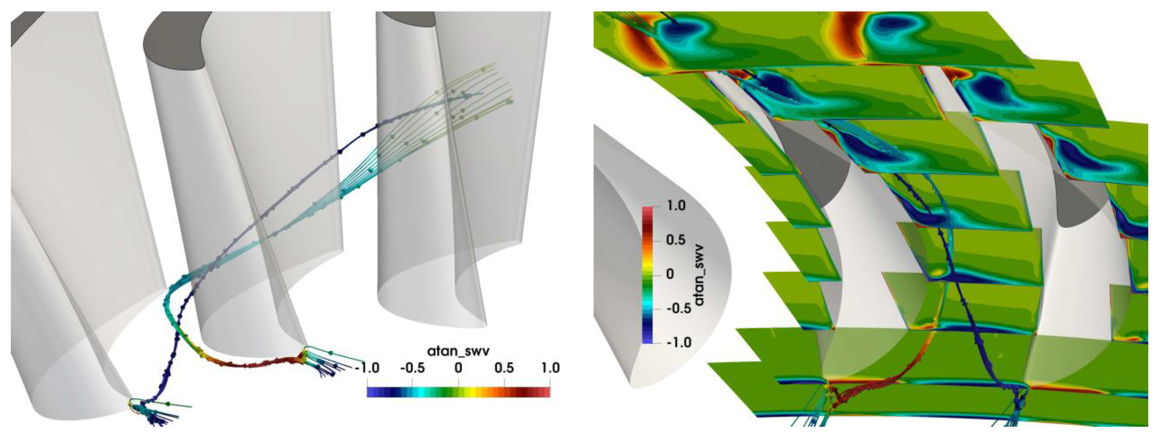
The flow in the tip region was dominated by the tip leakage vortex. In Figure 7 (left), the red streamlines coming from the pressure side and passing the tip gap and the blue slightly rotating streamlines coming from the leading edge formed together the tip leakage vortex. The diameter of the vortex increased in the aft section due to a strong backflow region in its center, as depicted in Figure 7 (right). In Figure 7 (middle), additional streamlines coming from the neighboring blade pressure side are turned towards mid-span by the tip leakage vortex, forming a strong counter-rotating vortex, the upper channel vortex. These secondary flows are also well seen in the SWV contours in Figure 8 (left). The tip leakage vortex (blue zone of counter-clockwise vorticity) formed after the leading edge and strongly grew in streamwise direction. The clockwise-rotating channel vortex wrapped around the tip leakage vortex and stretched towards mid-span. Figure 8 (right) shows the secondary flow at the channel outlet. The backflow zone dissolved, and a strong, but smaller, tip leakage vortex can be seen surrounded by the channel vortex.

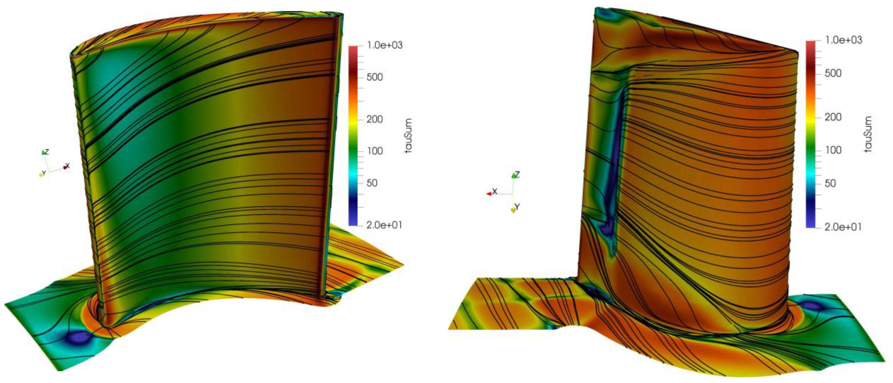
The effect of the described secondary flows can be clearly seen in the wall streamlines based on the wall shear stress on the rotor blade in Figure 9. On the pressure side, the flow moved towards the hub, driven by the lower channel vortex. In the tip region, there was a strong radial movement caused by the common effect of upper passage vortex and tip leakage flow. On the suction side, there was a distinct movement towards mid-span at hub and shroud. In the tip region, the limit streamline separated the counter-rotating tip leakage vortex and the upper channel vortex, as described above. A similar strong radial movement was found in the hub region. The small zone of low wall shear at mid-span indicated flow separation caused by the impinging shock there. Additional small backflow regions were found at the hub and tip.

4.3. Unsteady Velocity Field

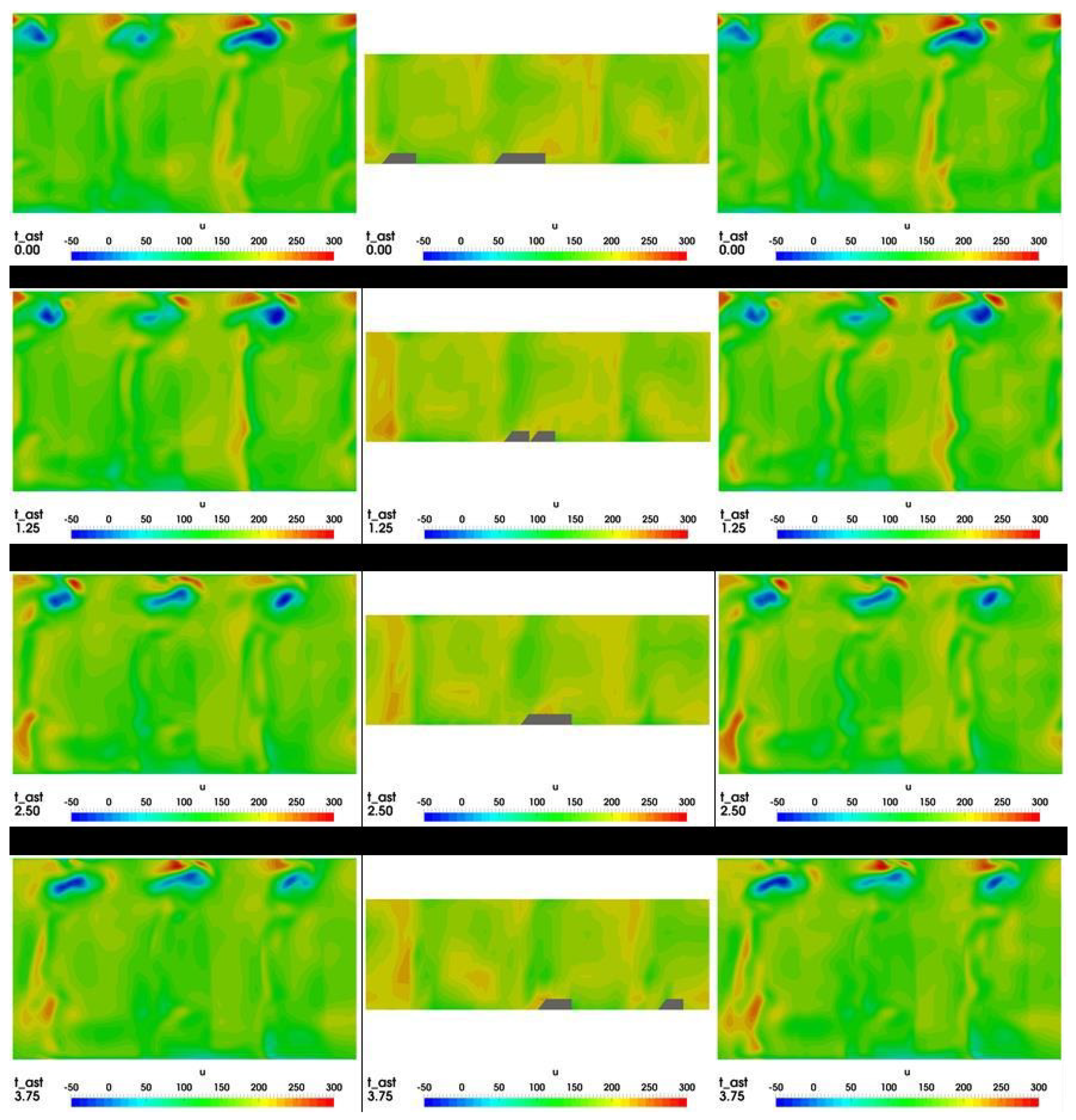
A comparison of the unsteady velocity field between measurements and simulation for plane C1 after the rotor is given in Figure 10. Results are shown for four time instants during 5 deg. of rotation, so that the flow repeats in the channel to the left. Simulation results are shown for turbulence inlet conditions of 18%/5 mm and 12%/1 mm to illustrate their influence. Looking at the simulation results, the three rotor wakes of lower velocity are slightly visible, moving from left to right. The flow differed remarkably between the three channels under the influence of the stator flow. The zone of higher velocity, clearly visible in the first two time instants, dissolves, whereas a new zone appears on the left in the next two time instants. In the shroud region, strong differences in velocity occurred, mainly due to the tip leakage flow. Zones of highest velocity appear close to the blue zones, indicating the backflow in the core of the leakage vortex, which varied strongly during the rotation. Comparing the numerical results of the two different turbulence inlet conditions, the main flow features were very similar, but slight differences regarding the backflow region, the shape of the wakes, and the zone of high velocity in the main flow can be clearly seen. Regarding the difference to the experimental results, it was larger than the one between the different turbulence conditions. The zone of high velocity was well predicted, but the phase lag already seen in Figure 4 and Figure 5, led to an earlier emergence of the high-velocity zone on the left side.

4.4. Unsteady Turbulence Prediction

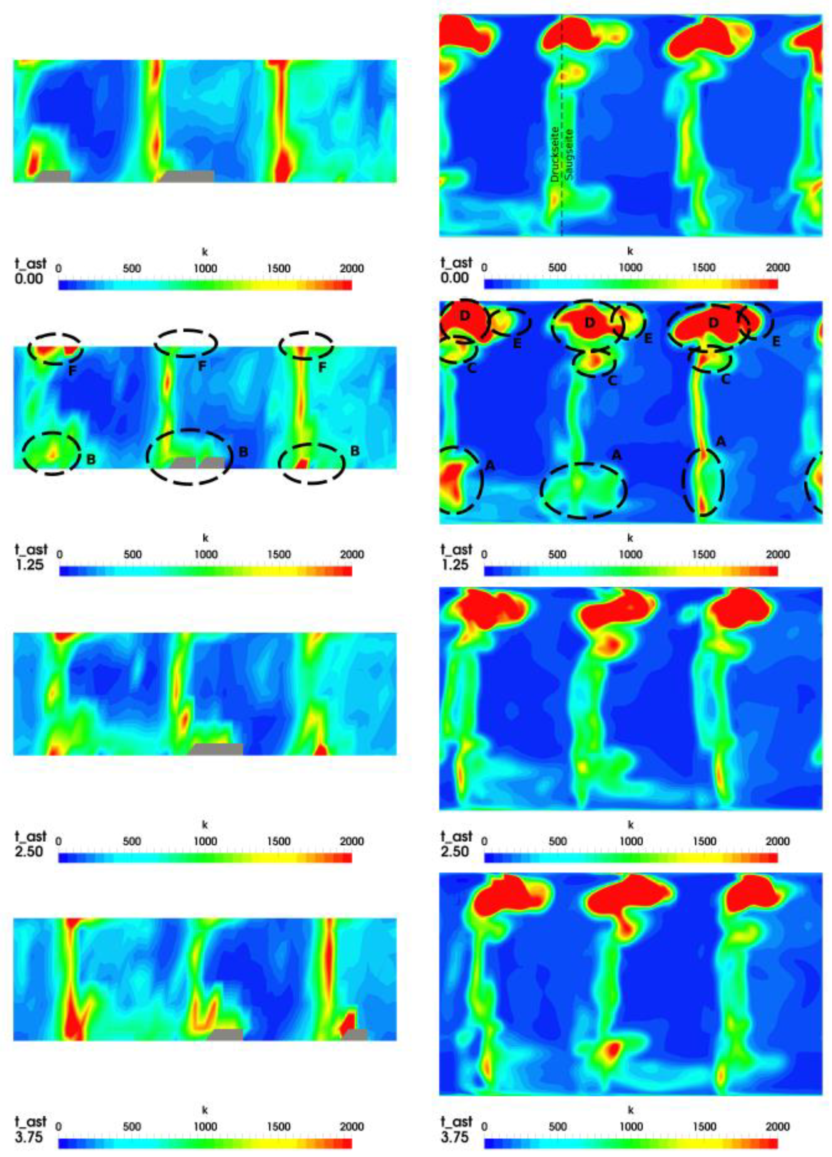
A comparison of the unsteady turbulence kinetic energy between measurements and simulation for the higher inlet turbulence case in plane C1 after the rotor is given in Figure 11. As shown in Figure 5, the predicted turbulence in the main flow was mostly lower than in the measurements, even considering the uncertainty of the measurements.

The maximum values in the wake flow were about half the ones in the measurements. The very high turbulence there can be explained with the secondary flows described above. Zone A at the hub came from the lower channel vortex and the trailing edge vortex sheet there. They remarkably varied in strength over time, due to the influence of the preceding stator blades. The corresponding zone B in the measurements was located slightly more towards mid-span.

In the tip region, the zones of high turbulence correspond to the zones of high SWV in Figure 8. The zones C and D in the predictions and corresponding zone F in the measurements can be explained by the interaction of tip leakage vortex and upper channel vortex, which generated further rotating structures in the outflow region. Again, the strong variations during the rotation were remarkable. The measurements also showed temporally high values in the wake region, which can only be partly found in the computations. Measured local maxima of turbulence in the mid-channel could not be predicted.

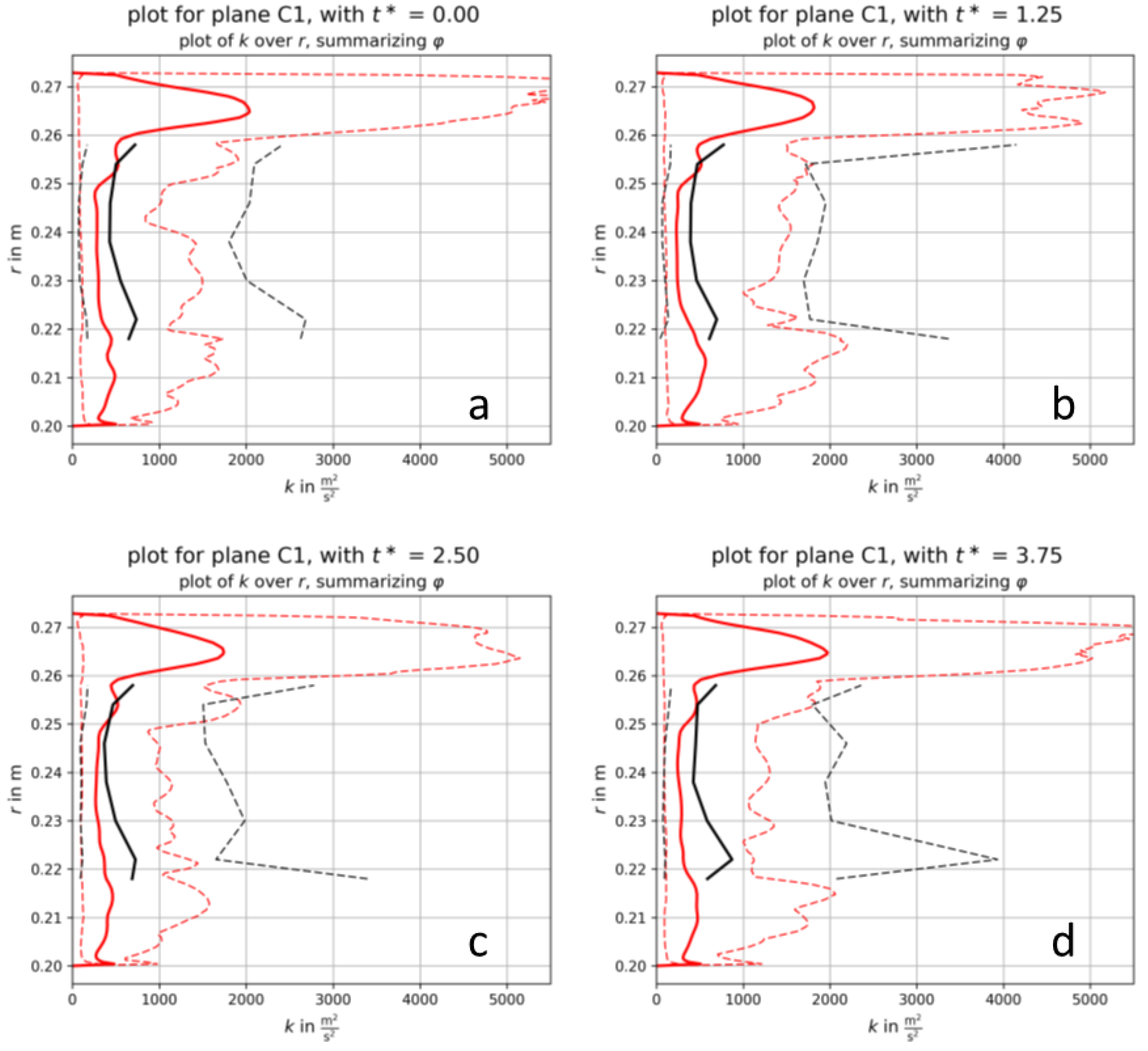
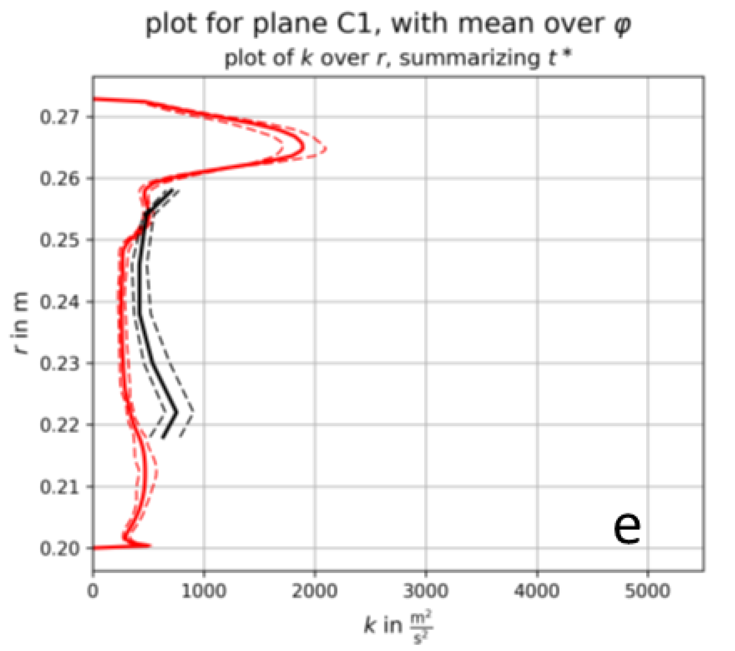
A more quantitative comparison of the unsteady turbulence after the rotor (plane C1) is given in Figure 12, where radial distributions of the circumferentially averaged turbulence kinetic energy are given for the experimental and computational data. Additionally, the minimum and maximum values at each time instant are displayed. At most radial positions the measurements showed a distinct higher averaged turbulence kinetic energy. The minimum values were nearly identical, whereas the maximum values were remarkably higher in the measurements at all time instants. Only in the outer region similar maxima occurred, indicating that the secondary flows extended more towards mid-span in the simulations. The highest turbulence values in the simulations appeared in the tip region, where the tip leakage vortex and the upper channel vortex interacted. Strong variations over time can be detected in this region. Figure 12e displays the time average and the temporal variations of the mean distributions, which were surprisingly small despite high local and instantaneous fluctuations.

5. Conclusions

An unsteady flow simulation of a transonic turbine stage was performed in order to study if an unsteady simulation can give a better agreement with the measurement data than steady simulations done in the past. The turbulence inlet boundary conditions were first varied in an unsteady Q3D simulation to see their influence. None of the boundary conditions could predict the free-stream turbulence level after the rotor or the maximum values of turbulence kinetic energy in the wake, whereas the stator free-stream value could be captured.

Regarding the secondary flow, it could be well captured by the unsteady 3D simulation, although the quantitative agreement was not satisfying. Luckily, the velocity field itself after the rotor was only slightly influenced by the inlet conditions of turbulence, so that especially the time-averaged solution should be independent of them.

Regarding turbulence, it was predicted very high in the shroud region where backflow occurs inside the tip leakage vortex. However, in the mid-span region, where measurements are available, the predicted values were lower in the free-stream as well as in the wakes. This indicated that a linear eddy viscosity model is not sufficient to model the intricate generation, destruction, and mixing out of turbulence in a complex turbine flow.