Article

Optimal Design of a Ljungström Turbine for ORC Power Plants: From a 2D model to a 3D CFD Validation

Department of Mechanical and Aerospace Engineering, University of Roma Sapienza, Via Eudossiana 18, 00184 Roma, Italy
*
Author to whom correspondence should be addressed.
Int. J. Turbomach. Propuls. Power 2020, 5(3), 19; https://doi.org/10.3390/ijtpp5030019
Submission received: 23 April 2020 / Revised: 3 July 2020 / Accepted: 14 July 2020 / Published: 20 July 2020

Abstract

:
In the last few years, waste-energy recovery systems based on the Organic Rankine Cycle (ORC) have gained increased attention in the global energy market as a versatile and sustainable technology for thermo-electric energy conversion from low-to-medium temperature sources, up to 350 °C. For a long time, water has been the only working fluid commercially adopted in powerplants: axial and, for smaller machines, radial inflow turbines have been the preferred expanders since their gulp capacity matches the ρ-T curve of water steam. The density of most organic compounds displays extremely large variations during the expansion (and the volume flow rate correspondingly increases along the machine channels), so that Radial Outflow Turbines (ROTs) have been recently considered instead of traditional solutions. This work proposes a two-dimensional inviscid model for the stage optimization of a counter-rotating ROT, known as the Ljungström turbine. The study starts by considering five different working fluids that satisfy both the gulp requirements of the turbine and the hot source characteristics. On the basis of a limited number of geometric assumptions and for a fixed set of operating conditions, different kinematic parameters are optimized to obtain the most efficient cascade configuration. Moreover, as shown in the conclusions, the most efficient blade profile leads to higher friction losses, making further investigation regarding the best configuration necessary.

1. Introduction

The research and development of the Organic Rankine Cycle (ORC), based energy conversion systems, is mainly aimed at the accurate prediction of the performance of the expander, which strongly influences the efficiency of the entire plant. Moreover, based on the characteristics of energy sources exploited by the plant, some expanders are more suitable than others, leading to a higher efficiency of the overall process.
With the exception of the smallest ORC power plants (few kW), where volumetric expanders of scroll and screw type can be used, whenever higher power outputs are needed, and consequently high expansion ratios and/or high volume flow rates are necessary, dynamic turbines are the only feasible expanders [1]. Tocci et al. [2], in their review of ORC for small scale applications, argue that the selection of the expander type in the range of power 20–70 kW represents an open question: on the one side, the size of volumetric expanders increases exponentially with an increment of output power [2], on the other, traditional radial inflow solutions may lead to unrealistic rotational speeds [3,4].
In light of the above, the purpose of this paper is to investigate the suitability of a special class of Ljungström turbines, specifically designed for the very large expansion rates of organic fluids in the range of power for which a preferred choice is not yet defined and consolidated. To do so, we will start from the study of the velocity triangles of a Ljungström type radial outflow turbine that exploits low-T thermal sources and produces significant power output [5] and then continue to their optimization.
The Ljungström turbine owes its name to its inventors, the Ljungström brothers, who in 1908 conceived, designed and produced a statorless steam turbine, as shown in Figure 1, consisting of two counter-rotating coaxial disks fitted with several concentric blade crowns [6]. The inlet section is located radially near the shaft while the outlet is at the outer radius at the exit of the last blade crown. This arrangement compensates for the increase in the volume of the fluid during the expansion by a corresponding increase in the flow area along the flow path.

2. Materials and Methods

2.1. Fluid Selection

In this work, a hydro-treated mineral oil, Paratherm NF, is the heat transfer medium taken as the hot source. It enters the boiler at 140 °C (413 K) with a mass flow rate of 4 kg/s. The cold source is water, which enters the condenser at room temperature (25 °C or 298 K) and is assumed to be available in the necessary quantity. The selection of the working fluid and the identification of the thermodynamic cycle was performed via a MATLAB code by using the CoolProp library [9] to calculate the fluid properties. A first selection of fluids from the CoolProp library was performed under two criteria: first, since the source is at low temperature, the fluid should have a low critical pressure [10,11]; second, the Ljungström turbine requires relatively high volume flow rates at its inlet and a well-identified variation in the density along the radius due to its peculiar cross-sectional area, and thus the fluid ought to have a low density at turbine inlet (i.e., high values of the coefficients in the Redlich–Kwong equation of state). According to these considerations the following fluids were considered: an alicyclic hydrocarbon, Cyclopentane (C5H10); an azeotropic mixture, SES36; a haloalkane refrigerant, R134a (CH2FCF3); an alkane refrigerant, R601 (C5H12); a hydrofluorocarbon refrigerant, R245fa (C3H3F5).
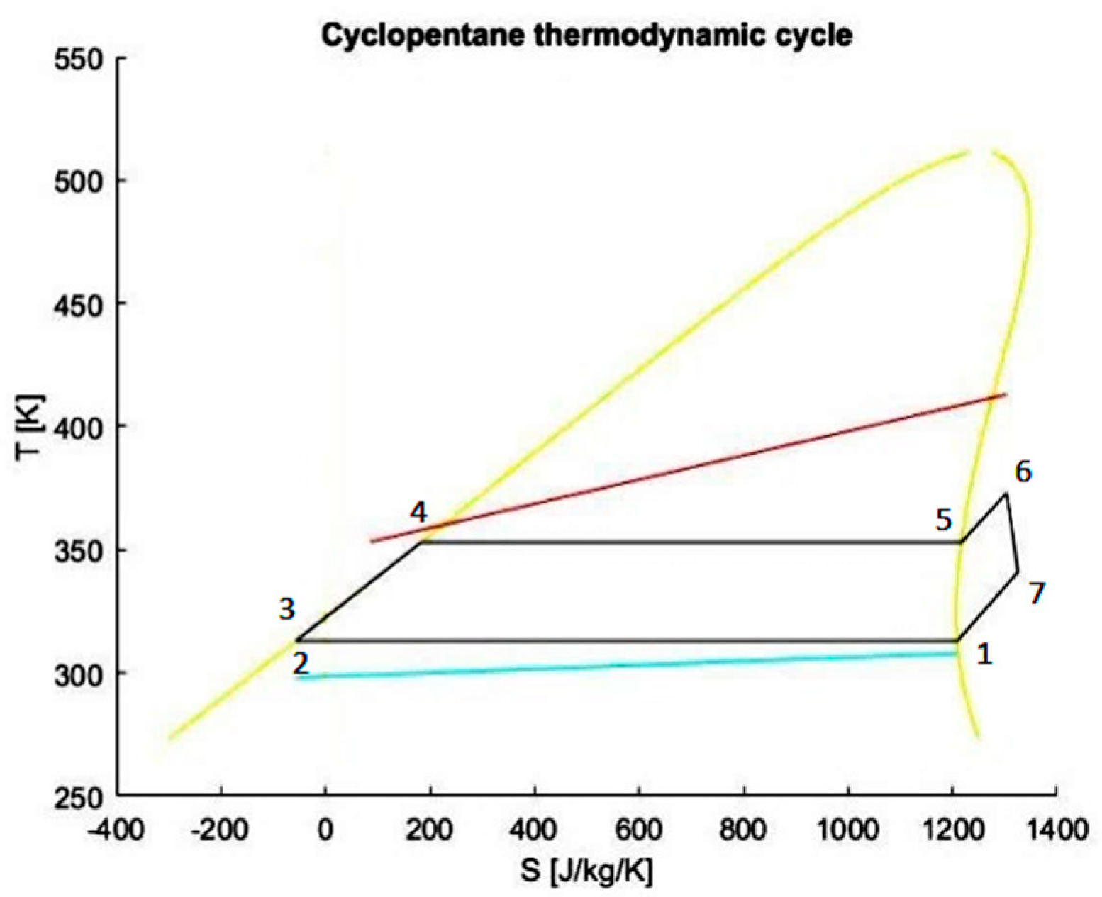
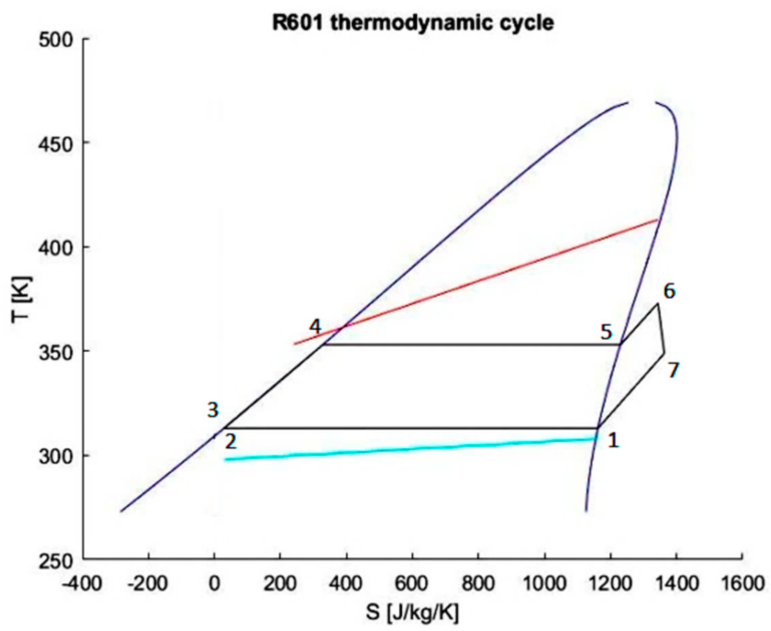
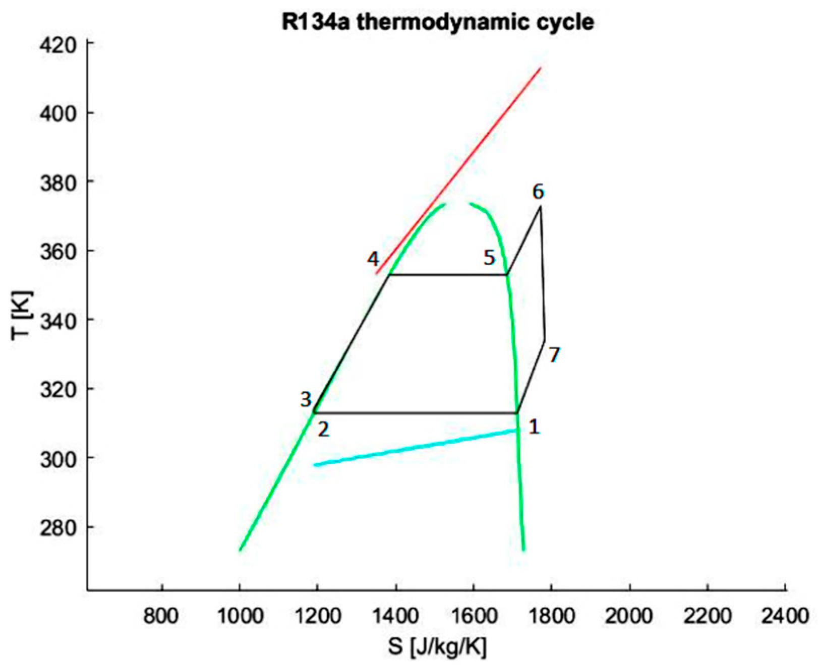
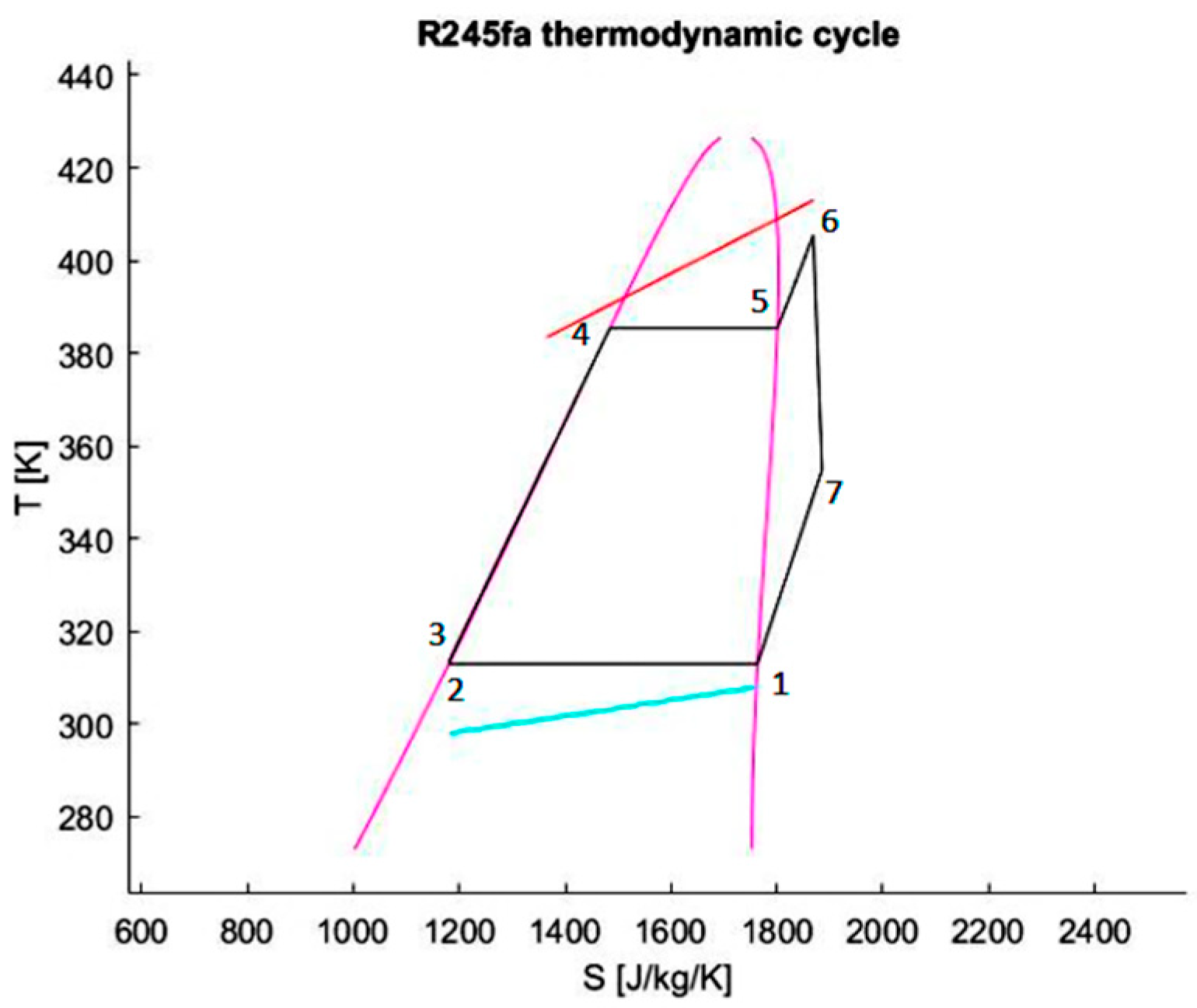
For each working fluid, as shown in Figure 2, a specific thermodynamic cycle was designed by fixing the top and bottom pinch points and specifying a 10 °C water temperature rise in the condenser. For a correct comparison, the thermal power input is the same for all cycles considered. The heat input and output in the boiler and the condenser were then matched by iteratively adjusting the working fluid mass flow rate or/and the evaporation temperature. Therefore, the turbine enthalpy drop and the pump work were determined with an assumed 0.8 efficiency for the pump and 0.83 (polytropic) for the turbine. The overall cycle efficiency is equal to:
η c y c = m ˙ w f ( L t u r b L p u m p ) m ˙ o i l Δ H o i l ,
Table 1, Table 2, Table 3, Table 4 and Table 5 present the thermodynamic properties of the considered fluids at the relevant stations in the process. Figure 3, Figure 4, Figure 5, Figure 6 and Figure 7 clearly show that, in all of the cycles, a regenerator recovers a portion of the sensible heat content of the working fluid before it enters the condenser. The percentage of thermal power recovered by the regenerator amounts to 7.98% of the whole thermal input for the Cyclopentane, 14.50% for the R601, 11.23% for the R134a, 15.99% for the R245fa and 21.42% for the SES36. Efficiencies and mass flow rates (indicative of expander size) are reported in Table 6.

2.2. The Optimization Algorithm

The standard formulation of the Euler work (2) shows that, for a Ljungström “stage”, the only positive contribution to the specific work is given by the increase in the relative velocity, because uout is only slightly higher than uin:
L E u l = v 2 i n v 2 o u t + u 2 i n u 2 o u t + w 2 o u t w 2 i n 2 ,
The novel method for the mean-line design proposed here begins with the following two positions, first suggested by Kearton [12] and Shepherd [13]:
  • All blades, except those in the innermost ring, have the same cross-section, the same profile and the same stagger angle and, as a consequence, also have the same outlet angle:
    β o u t = c o n s t . ,
  • In all blade crowns, the ratio of the relative outlet steam velocity to the peripheral velocity at the outlet edge of the blade ring is constant and equal to:
    ρ r = u o u t w o u t < 1 ,
  • In all blade crowns, the ratio of the radial chord of the blade to the outlet radius is constant and equal to:
    χ = 1 b r o u t = r i n r o u t < 1 ,
  • Due to the axial symmetry of the turbine, the absolute velocity at the inlet of the first row can be considered completely radial.
The above assumptions suffice for a definition of kinematic efficiency. Since the relative velocity provides the only positive contribution to the Euler’s work, the absolute velocity and the peripheral velocity are to be considered as losses, and this leads to the following formula:
η k i n = 1 v o u t 2 v i n 2 + u o u t 2 u i n 2 w o u t 2 w i n 2 ,
That can be rewritten as:
η k i n , i = 1 ( 1 χ 2 ) · ( 1 + 2 ρ r 2 2 ρ r cos β o u t ) 1 χ 2 · ( 1 + 4 ρ r 2 4 ρ r cos β o u t ) ,
This equation provides additional useful information because it is similar for every i-th blade ring except for the first one, where it takes the following form:
η k i n , 1 = 1 ρ r 2 ( 2 χ 2 cos β 0 2 ) + 1 2 ρ r cos β o u t 1 χ 2 cos β 0 2 ,
The parameters to be considered to maximize the kinematic efficiency are, therefore, ρr, χ, βout and β0. Due to the second and third assumptions it is not possible to maximize both ηkin,i and ηkin,1 with respect to ρr and χ, thus only the ηkin,i equation is considered here for the optimization.
It can be easily verified that the derivative of the kinematic efficiency (7) is linearly dependent on both χ and βout and thus it is not possible to maximize this equation with respect to these parameters. This conclusion is reinforced by a closer inspection of Equation (7), which is maximized either when the numerator of the second term tends to zero or the denominator to a maximum. Both cases leading to ideal turbine configurations:
  • χ = 1, meets the maximum of the efficiency for ρr = cos(βout)/2, and causes the numerator to be null. In fact, in this case uin = uout and vin = vout so that the velocity triangle is similar to that of an impulse turbine;
  • βout = 0 causes the denominator to be at its maximum, in which case win = 0 because the triangle collapses onto a line.
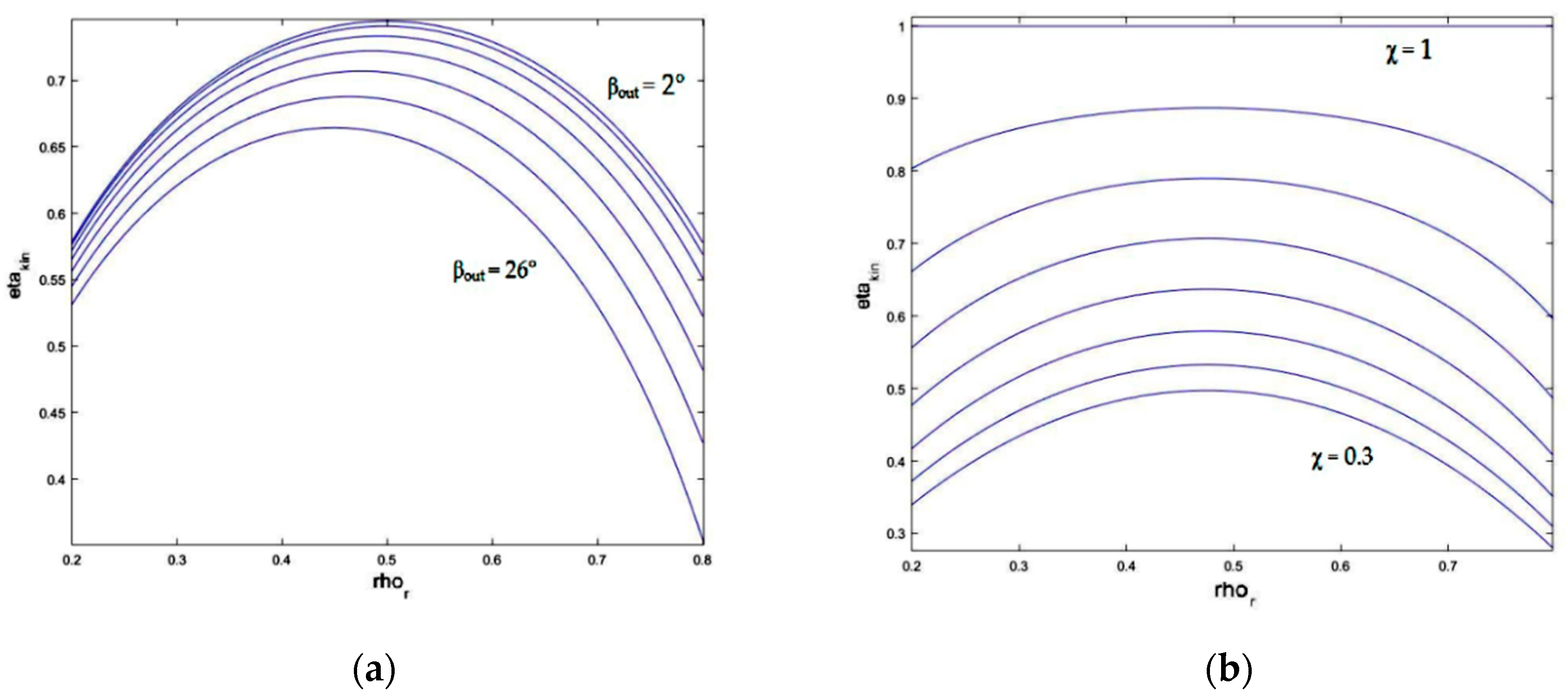
Therefore, the only parameter to be considered in the velocity triangles optimization is ρr, which allows us to maximize the kinematic efficiency for different values of βout and χ, as shown in Figure 8.
Considering the above, we can now proceed to the study of the isentropic efficiency, starting from its equation and the loss model adopted here:
Δ h s s = w o u t , i d 2 w i n 2 ( u o u t 2 u i n 2 ) 2 ,
In order to obtain the value of wout,id, Soderberg [14] loss correlation was used:
w o u t , i d = w o u t 1 + ξ r ,
And after some rearrangement, the formula of the isentropic efficiency for the i-th row, with the exception of the first one, is obtained:
η i s , i = 2 ( 1 + χ 2 ) ρ r cos β o u t ρ r 2 ρ r 2 1 + ξ r , i ρ r 2 1 + χ 2 ( 1 1 + ξ r , i 1 + 4 ρ r 2 4 ρ r 1 + ξ r , i 1 cos β o u t ρ r 2 ) ,
While for the first row:
η i s , 1 = 2 ρ r cos β o u t ρ r 2 ρ r 2 1 + ξ r , 1 ρ r 2 1 + χ 2 ( 1 1 cos β 0 2 ) ,
The Soderberg loss coefficient is adopted for all the ensuing calculations, but different models were tested as well, such as Ainley and Mathieson [15] and Craig and Cox [16] prediction models. With little modifications in the code, the loss coefficient ξr can be evaluated for any of the abovementioned prediction models. It was found that the adoption of different loss models does not noticeably influence the results, as shown in Figure 9.
Since ξr depends on the fluid dynamic and geometric conditions that are different in each row, it is not possible to choose a single value of ρr for all rows that optimizes ηis,i. This justifies the choice of a velocity triangles optimization based on the selection of the ρr that maximizes the ηkin,i.
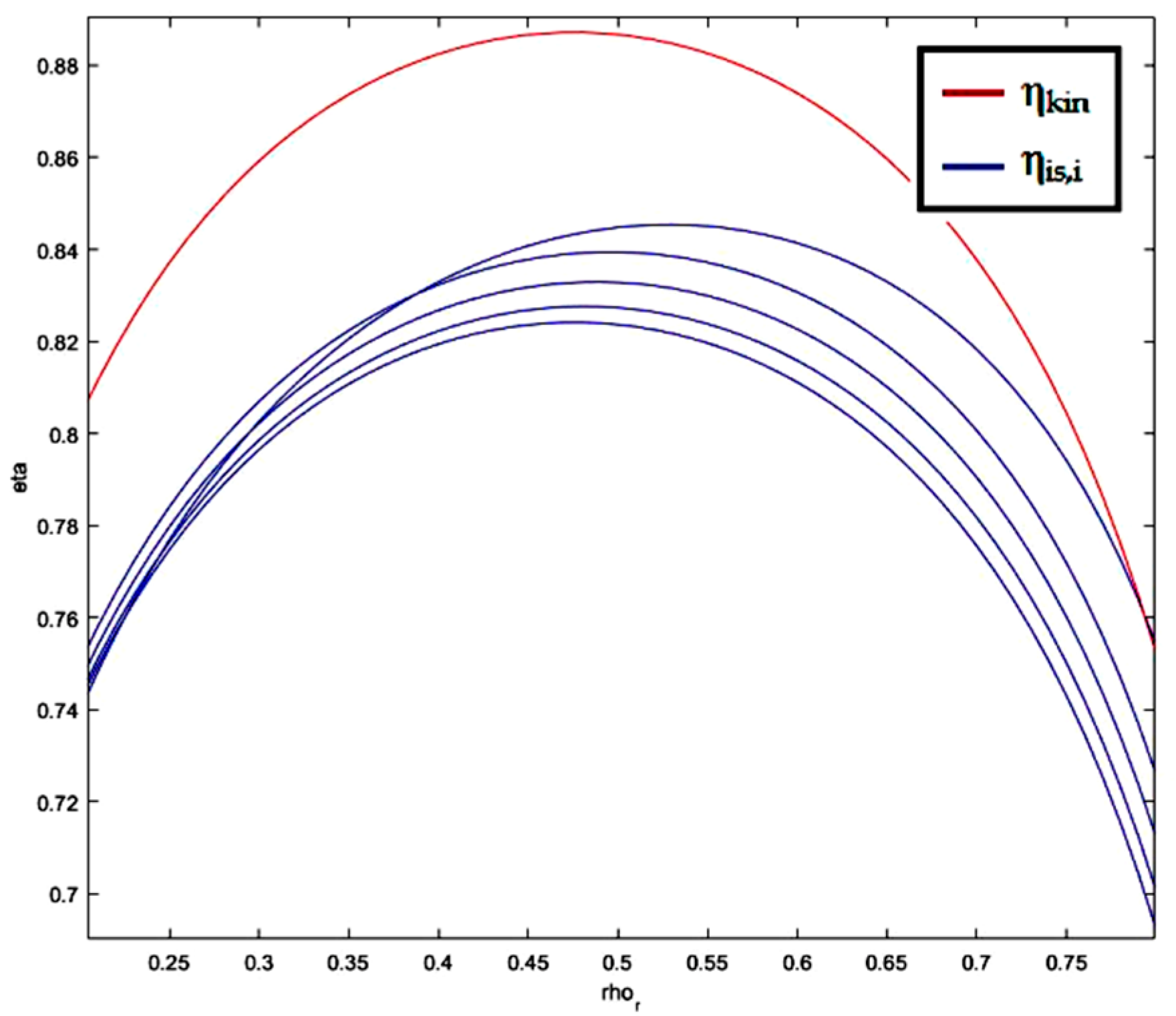
As shown in Figure 10, for a fixed geometry (fixed χ and βout) and by varying the velocity, and consequently ξr, the maximum of the isentropic efficiency is close to the range of the maxima of the kinematic efficiency. This supports the choice of an optimization procedure based on the velocity triangles.
A MATLAB code was written to obtain a complete mean line analysis, and then the flow in the resulting geometry was simulated via a CFD analysis to validate the model. The inputs of the algorithm are shown in Table 7.
By setting a trial rotational speed ω = ωmax the shaft diameter can be found that sets a lower limit to the inlet radius at the entrance of the first row. Thence we obtain a matrix of all possible combinations of rin and βin that satisfy the continuity equation for all the l > lmin.
The abovementioned matrix leads to another matrix of all possible values of ηkin. By taking the maximum value we can also find the optimal values of ρr and χ. With all these parameters in place, it is now possible to calculate the loss coefficient ξr and the enthalpy drop for the first stage (∆hi).
i = 1 n ° r o w s h i = h t o t ,
If (13) is not satisfied it is possible to design additional rows and if an exact match is not achieved, a modified rotational speed ω = ωmax − ∆ω is selected and the process is iteratively repeated, as shown in Figure 11.
Since the maximum efficiency is reached for b = 0 and βout = 0 and since these conditions are clearly unphysical, a minimum value must be arbitrarily specified. In addition, the change of the cross-sectional area along the radius requires the designer to specify a minimum value of the axial blade length at the inlet:
h m i n = ξ · m ˙ w f 2 π ω r i n 2 ρ tan β 0 δ b ,
where the leakage factor ξ was assumed here to be 0.98.
The above equation has two degrees of freedom. By fixing a proper range of values for β0 and rin all possible combinations that meet the equation can be calculated. These ranges are constrained by two different conditions. β0 must be limited in order to obtain wout,1 > win,1:
0 < β 0 < cos 1 ( χ ρ r 1 1 + ρ r 2 2 ρ r cos β o u t + χ 2 ρ r 2 ) ,
while rin for the first row must be larger than the shaft radius that was calculated with the following formula:
d s h a f t K 16 P π ω 3 ,
where K = 1.3 is a safety factor, P [MPa] the power at the shaft and ω [rpm] its rotational speed [17]. Subsequently the code designs the first row using the inputs provided by the optimization function. It starts from the velocity triangles, calculates the isentropic heat drop using the loss coefficients and finally derives the thermodynamic quantities at the outlet of the row. The quantities thus derived are used as inputs for the following stage, leading to an iterative process.
The proposed algorithm leads to a choice in the number of stages as a function of the maximum angular speed.
h m i n = ξ · m ˙ w f 2 π · ω · r i n 2 · ρ · tan β 0 . δ b ,
As shown in Table 8 and, as expected, the χ parameter is strictly correlated to the efficiency of the turbine. A closer look to these results reveals that the less efficient thermodynamic cycles presents the higher isentropic efficiencies. The Ljungström turbine performs better with low enthalpy drop and high-volume flow rates (higher specific speed ns). Moreover, since the cross-sectional area depends on the volume flow rate variation, not all the selected fluids lead to geometrical characteristics, such as axial blade length, which correspond to the allowed manufacturing limits. As shown in Table 9, the only suitable fluids are Cyclopentane and R601, the only ones leading to an axial blade length acceptable for the imposed constraints.
In the present study, R601 was chosen as working fluid because, despite the slightly lower efficiency of its cycle, it is much less flammable than Cyclopentane. Moreover, its condenser pressure is about 1 bar against 0.7 bars for Cyclopentane, making the manufacturing easier.
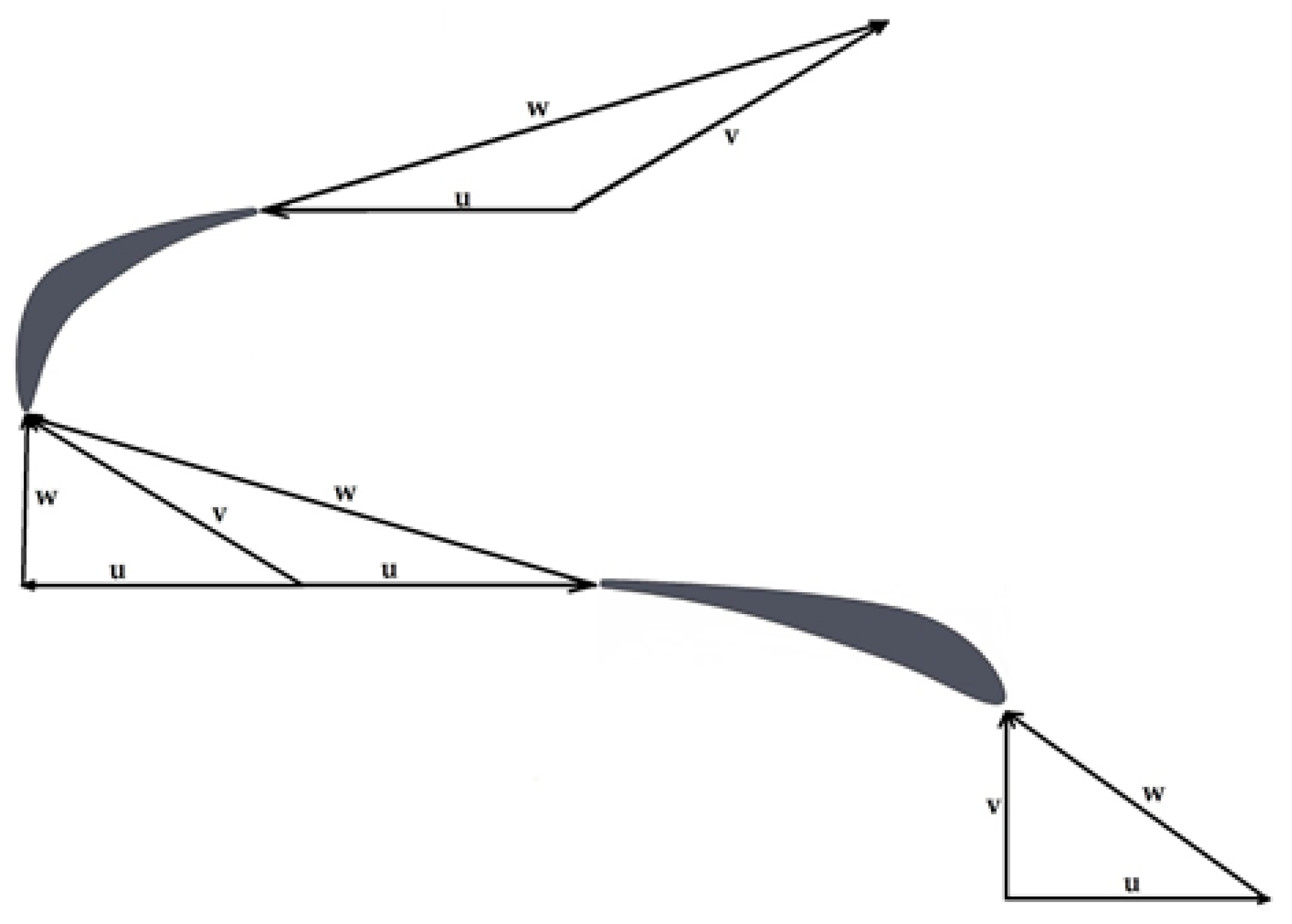
The design parameters thus obtained, as shown in Table 10, make it possible to draw the velocity triangles of the best performing configuration, as shown below in Figure 12:

3. Results

CFD Validation

The configuration proposed in Figure 12 was simulated via a viscous turbulent CFD analysis, to validate the proposed model. The blade shape was designed using Dunham’s parametric method [18] and the number of blades was selected using a modified Zweifel’s criterion [19,20], since ROTs have an axial blade shape. A MATLAB code based on the above parametric method was written to define the shape of the blades by interpolating over 1000 points chordwise; then the blade shape was imported in SolidWorks and simulated by Ansys Fluent.
For the CFD simulation a RANS model with a kε turbulence model was used. For this preliminary design validation, the viscous sublayer was not resolved. Both two- and three-dimensional simulations were performed. The relative motion was simulated by the sliding mesh method in the two-dimensional case and by the Multiple Reference Frame (MRF) model in the three-dimensional case.
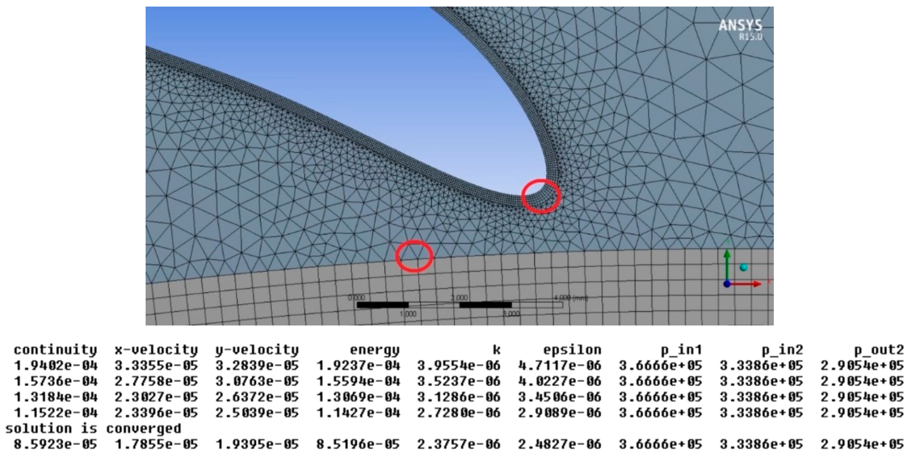
A Conformal Mesh was generated using a growth rate of 1.045 in order to have a mesh continuity as gradual as possible with triangular elements, except in the near-wall region where rectangular elements provide better accuracy. A mesh sensitivity analysis was performed (see Figure 13 and Figure 14) to check the independency of the results from the mesh generated. The objective function for the mesh sensitivity was the total entropy.
The above settings led to an acceptable number of nodes for an accurate two-dimensional study (200,862 nodes and 387,202 elements) and a y+ from 40 to 150 along the blade surfaces. By the same line of reasoning, we obtained 2.6 million hexahedral elements for the 3D study.
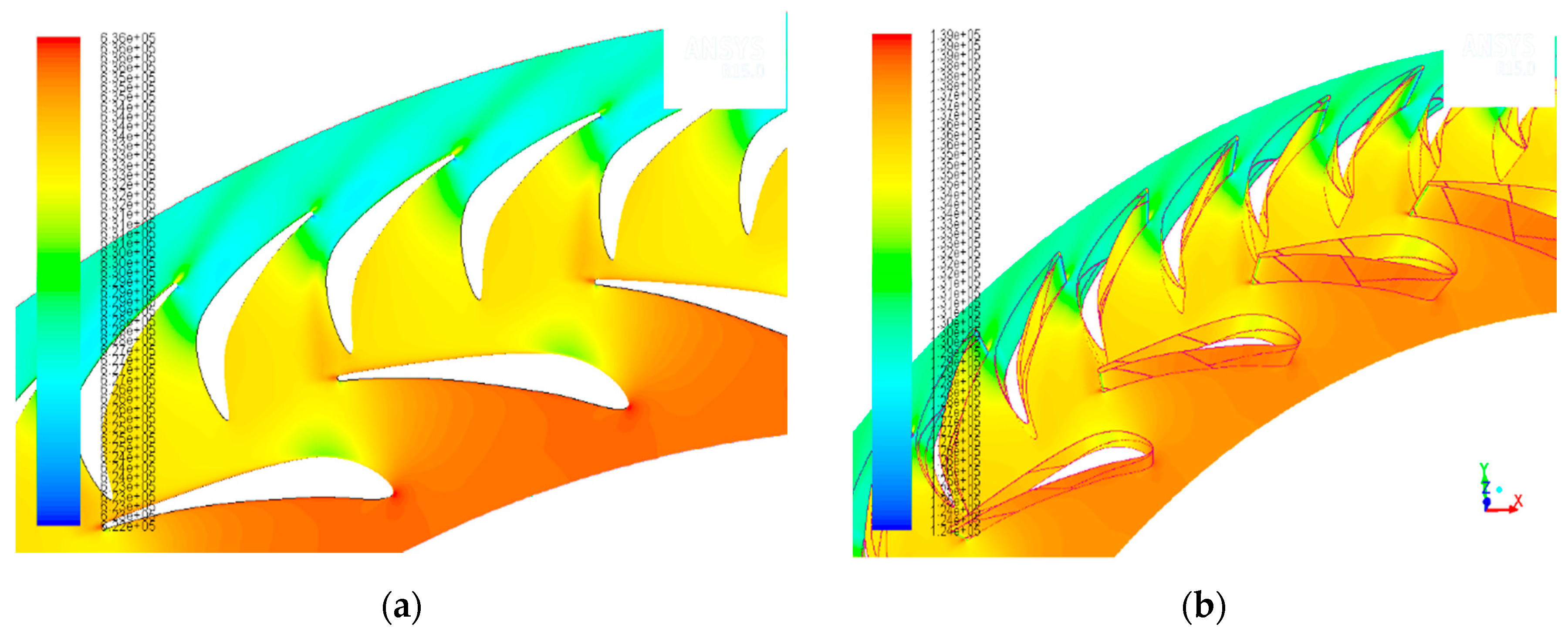
After a satisfactory convergence was obtained with a residual norm of the order of 10−5, different thermodynamic quantities were extracted from the numerical solution and compared with the analytic model, as shown in Figure 15. The output torque was calculated at each time step of the two- and three-dimensional simulations, to compare the power output with the model prediction.
Figure 16 shows the output power for both rows in all the analyzed cases. The continuous lines represent the model prediction, while the dashed lines represent the 2D configuration and the dotted lines are their averages. The asterisks represent the 3D configuration which was analyzed in a single frame.
The isentropic efficiency of the whole turbine is about 0.82; however, to make a comparison with the CFD results, only the first two rows are to be considered. Therefore, the isentropic efficiency decreases to 0.759 because of the low efficiency of the first row. For the 2D configuration, the efficiency for the first two rows, calculated on the basis of the average power and enthalpy drop, is about 0.762—for the 3D configuration, about 0.751. The reduction in efficiency from the 2D to the 3D configuration is caused by the increase in the frictional losses, in particular in the hub and tip boundary layers. In fact, since the Soderberg loss model takes into account 3D losses, the slightly higher value of the efficiency in the 2D analysis compared with the “analytical” efficiency can be attributed to the neglection of wall friction (on the disks), which are instead considered in the 3D analysis.
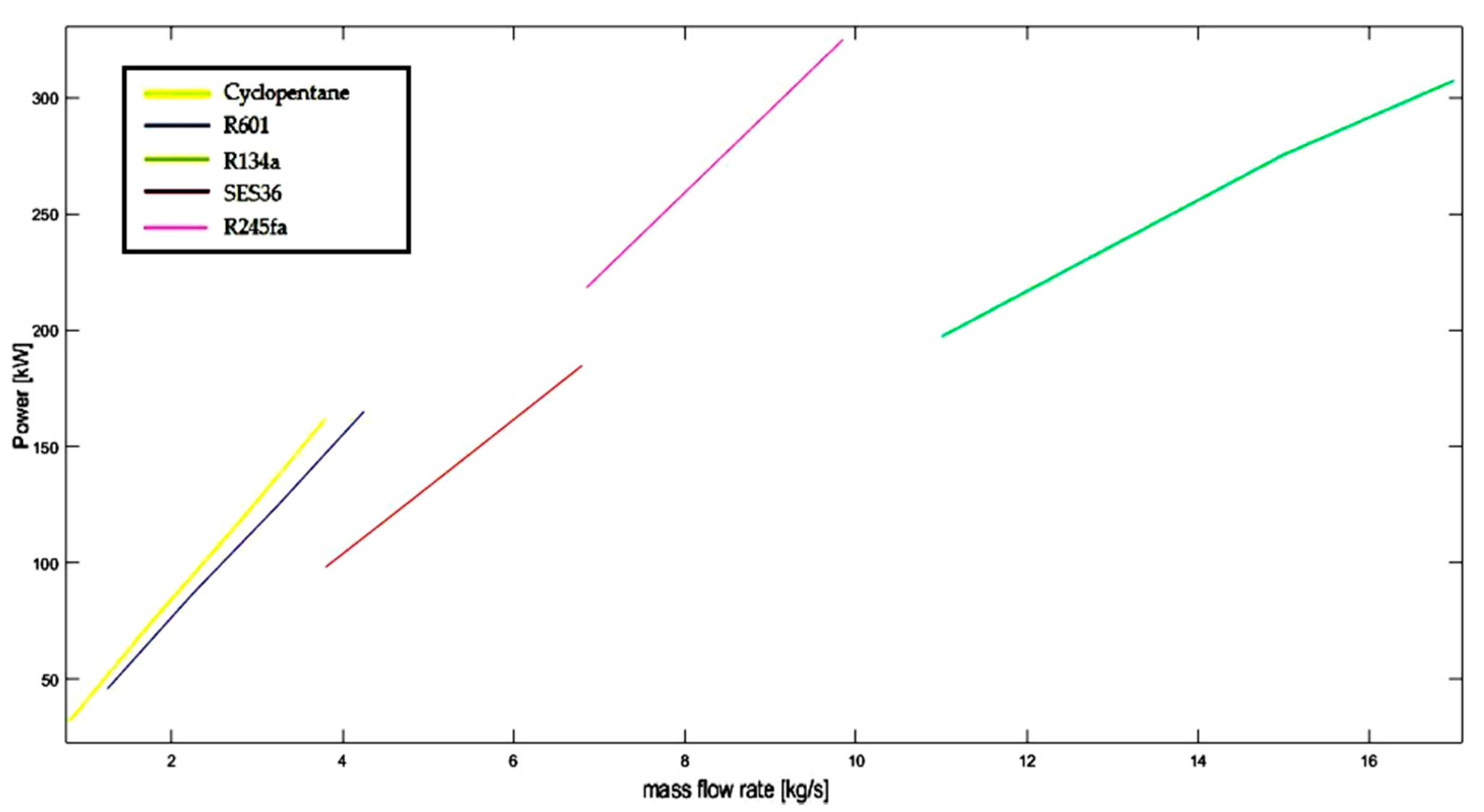
Now that the effectiveness of the proposed design algorithm has been demonstrated via the above described CFD simulations, it is possible to formulate an educated assessment of the suitability of the Ljungström turbine for different low-T thermal sources by using different working fluids in different ranges of power:
Figure 17 clearly shows that, as the range of power increases, higher density working fluids are required to match the Ljungström turbine characteristics.

4. Conclusions

To the best of our knowledge, there is not a commercially available Ljungström blade design software, and therefore the present study proposes the use of the kinematic efficiency as a new relevant design parameter in the Ljungström design. However, as discussed in Section 2, such a choice opens up a lot of points worthy of further discussion and investigation. The main reason is that this procedure does not take into account the centrifugal forces (absent in axial flows), and therefore the “optimality” of the blade profile proposed by the analytical model must be verified by an experimental validation. In the case studied here, this validation was obtained by a series of 2D time-dependent and by a steady state 3D CFD simulations. Though a full picture of the time evolution of the 3D flow is not available, nevertheless, some useful considerations can be drawn.
As clearly shown in Table 9, the axial blade length is a crucial parameter in Ljungström design. By looking at Equation (17), it is clear that once all parameters, except for density, are fixed, in fact the inlet radius of each row is determined by the assumption of a fixed radius ratio, while the flow coefficient is fixed by the assumption of a constant outlet angle. In light of the above, it is also clear that the axial blade length depends on the mass flow rate and on the enthalpy drop.
Following Shepherd and Kearton, it was assumed that all blades, except those in the innermost ring, have the same cross-section and they are all set similarly in the rotor. Some authors question the adequacy of these assumptions, used in the past for the design of large scale steam-powered ROT, since they lead to geometrical optimization instead of maximizing the isentropic efficiency [7]. According to these authors, if one removes the assumptions of constant βout and χ, it is possible to exploit two additional degrees of freedom for the axial blade length Equation (17). As a consequence, the formula of the kinematic efficiency changes its structure so that a multi-dimensional optimization is required.
Some existing designs split the turbine into a high pressure and a low pressure stage to avoid the reduction in axial blade length in the downstream blade crowns of the turbine. This alternative solution consists of a small reduction in the mass flow rate at the inlet (first stage) and an additional injection in the low pressure wheel; however, this is not in contrast with our model, although further investigations could be useful.
Clearly all the proposed changes should be analyzed in more depth because none of the above is supported by calculations. The method we propose is based on kinematic efficiency maximization, while isentropic efficiency determines the turbine performance. Even though ηkin does not take into account fluid dynamic losses, it is maximized with respect to ρr, the ratio between inlet and outlet radii. The latter also plays a major role in the axial blade length Equation (17). In the end, the shorter the blade length, the larger the wall friction losses and the lower the isentropic efficiency.

Author Contributions

Conceptualization, U.C. and E.S.; Formal analysis, U.C.; Investigation, U.C.; Methodology, U.C.; Supervision, E.S.; Validation, E.S.; Writing—original draft, U.C.; Writing—review and editing, E.S. All authors have read and agreed to the published version of the manuscript.

Funding

This research received no external funding.

Conflicts of Interest

The authors declare no conflict of interest.

Nomenclature

SymbolDescriptionUnit of MeasureSymbolDescriptionUnit of Measure
bradial chord[m]Vabsolute flow velocity[m/s]
cspecific heat[J/(kgK)]Wrelative flow velocity[m/s]
dsspecific diameter wfworking fluid
dshaftshaft diameter[m]woworking oil
haxial blade length/
enthalpy
[m]
[J/kg]
β0relative inlet angle
idideal βrexpansion ratio
ininlet δbblade encumbrance
lblade chord[m]εdeviation angle
Lwork[J/kg]ηcyccycle’s efficiency
LEulEuler’s work, [J/kg][J/kg]ηisisentropic efficiency
ltlength scale, [m][m]ηkinkinematic efficiency
m ˙ mass flow rate[kg/s]ηturbturbine efficiency
nsspecific speed ξleakage factor
outoutlet ξrSoderberg loss coefficient
ppressure[Pa]ρdensity[kg/m3]
Ppower[kW]ρrblade to relative outlet velocity ratio
rradius[m]σblade solidity
ReReynolds number τallallowable stress[MPa]
sentropy[J/(kgK)]φflow coefficient
s-sstatic-to-static χinlet to outlet radii ratio
Ttemperature[T]ψload coefficient
Ublade peripheral velocity[m/s]ωangular velocity[rpm]

References

  1. Quoilin, S.; van den Broek, M.; Declaye, S.; Dewallef, P.; Lemort, V. Techno-economic survey of Organic Rankine Cycle (ORC) systems. Renew. Sustain. Energy 2013, 22, 168–186. [Google Scholar] [CrossRef] [Green Version]
  2. Tocci, L.; Pal, T.; Pesmazoglou, I.; Franchetti, B. Small Scale Organic Rankine Cycle (ORC): A Techno-Economic Review. Energies 2017, 10, 413. [Google Scholar] [CrossRef]
  3. Kang, S.H. Design and experimental study of ORC (Organic Rankine Cycle) and radial turbine using R245fa working fluid. Energy 2012, 41, 514–524. [Google Scholar] [CrossRef]
  4. Pei, G.; Li, Y.; Ji, J. Performance evaluation of a micro turbo-expander for application in low-temperature solar electricity generation. J. Zhejiang Univ. 2011, 12, 207–213. [Google Scholar] [CrossRef]
  5. Palumbo, C.F.; Barnabei, V.F.; Preziuso, E.; Coronetta, U. Design and CFD analysis of a Ljungstrom turbine for an ORC cycle in a waste heat recovery application. In Proceedings of the ECOS 2016, Portorož, Slovenia, 19–23 June 2016. [Google Scholar]
  6. Ljungström, F. The Development of the Ljungström Steam Turbine and Air Preheater. Proc. Inst. Mech. Eng. 1949, 160, 211–223. [Google Scholar] [CrossRef]
  7. Casati, E.; Vitale, S.; Pini, M.; Persico, G.; Colonna, P. Centrifugal Turbines for Mini-Organic Rankine Cycle Power Systems. J. Eng. Gas Turbine Power 2014, 136, 122607. [Google Scholar] [CrossRef]
  8. Pini, M.; Persico, G.; Casati, E.; Dossena, V. Preliminary design of a centrifugal turbine for ORC applications. In Proceedings of the First International Seminar on ORC Power Systems, Delft, The Netherlands, 22–23 September 2011. [Google Scholar]
  9. Bell, I.H.; Wronsky, J.; Quoilin, S.; Lemort, V. Pure and pseudo-pure fluid thermophysical property evaluation and the open-source thermophysical property library CoolProp. Ind. Eng. Chem. Res. 2014, 53, 2498–2508. [Google Scholar] [CrossRef] [PubMed] [Green Version]
  10. Franchetti, B.; Pesiridis, A.; Pesmazoglou, I.; Sciubba, E.; Tocci, L. Thermodynamic and technical criteria for the optimal selection of the working fluid in a mini-ORC. In Proceedings of the ECOS 2016, Portorož, Slovenia, 19–23 June 2016. [Google Scholar]
  11. Drescher, U.; Brüggemann, D. Fluid selection for the Organic Rankine Cycle (ORC) in biomass power and heat plants. Appl. Therm. Eng. 2007, 27, 223–228. [Google Scholar] [CrossRef]
  12. Kearton, W.J. Steam Turbine Theory and Practice: A Textbook for Engineering Students; I. Pitman & Sons: London, UK, 1958. [Google Scholar]
  13. Shepherd, D.G. Principles of Turbomachineryi; Macmillan Pub Co.: New York, NY, USA, 1961. [Google Scholar]
  14. Soderberg, C.R. Unpublished Notes; Gas Turbine Laboratory, Massachusetts Institute of Technology: Cambridge, MA, USA, 1949. [Google Scholar]
  15. Ainley, D.G.; Mathieson, G.C.R. An Examination of the Flow and Pressure Losses in Blade Rows of Axial-Flow Turbines; HM Stationery Office: London, UK, 1951. [Google Scholar]
  16. Craig, H.R.M.; Cox, H.J.A. Performance Estimation of Axial Flow Turbines. Proc. Inst. Mech. Eng. 1971, 185, 407–424. [Google Scholar] [CrossRef]
  17. Sciubba, E. Lezioni di Turbomacchine; Euroma La Goliardica: Rome, Italy, 2001. [Google Scholar]
  18. Dunham, J. A Parametric Method of Turbine Blade Profile Design. In Proceedings of the ASME International Gas Turbine Conference and Products Show, Zurich, Switzerland, 30 March–4 April 1974. [Google Scholar]
  19. Zweifel, O. Optimum Blade Pitch for Turbo-Machines with Special Reference to Blades of Great Curvature. Eng. Dig. 1946, 7, 358–360. [Google Scholar]
  20. Pini, M.; Persico, G.; Casati, E.; Dossena, V. Preliminary design of a centrifugal turbine for ORC applications. J. Eng. Gas Turbines Power 2013, 134, 042312. [Google Scholar] [CrossRef]
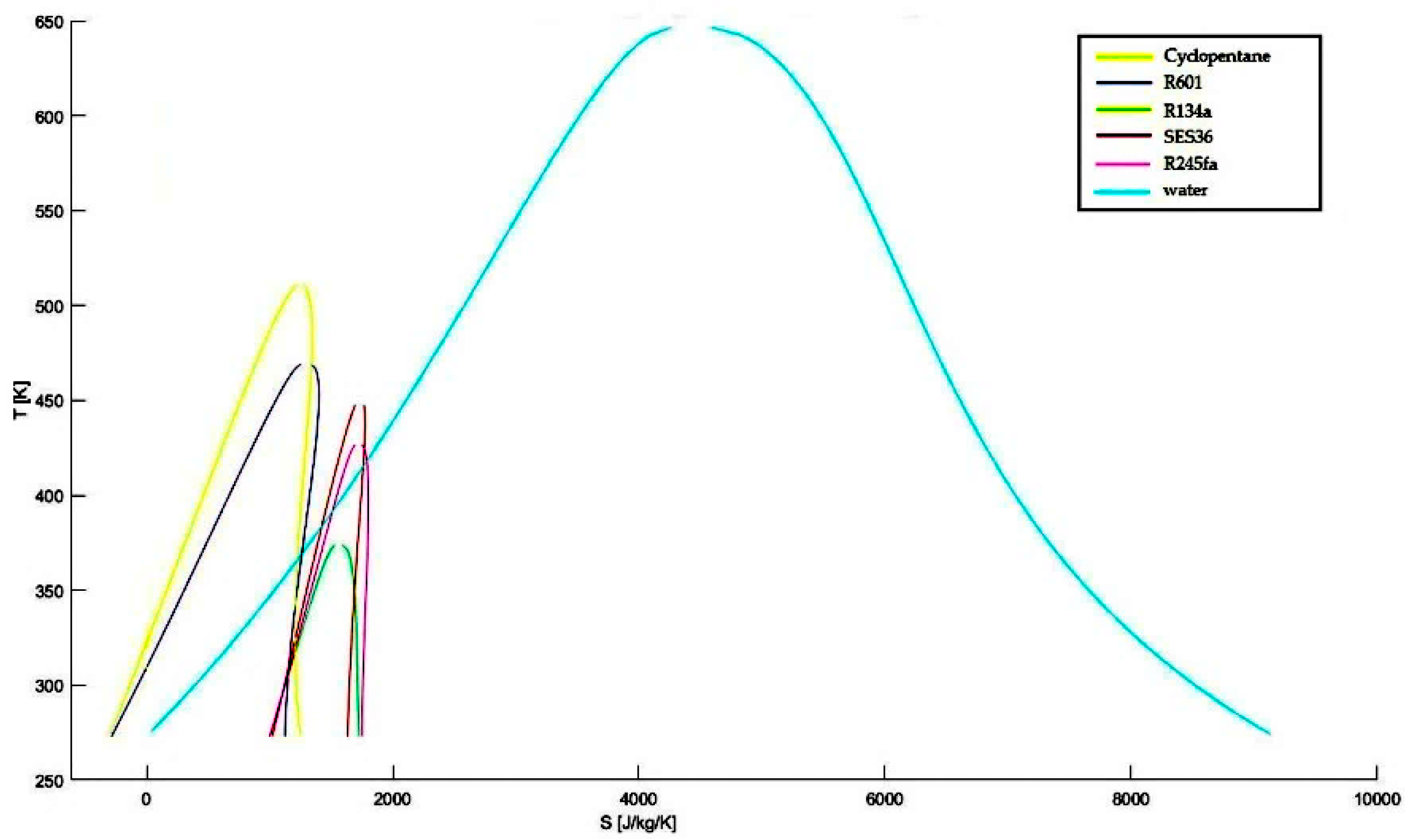
Figure 1. Ljungström Radially Outward Turbine (ROT): Fixed and Counter-rotating arrangements [7,8].
Ijtpp 05 00019 g001
Figure 2. Temperature–entropy diagram for the fluids considered in this study fluids, in the same scale as the usual water Mollier diagram.
Ijtpp 05 00019 g002
Figure 3. Cyclopentane TS diagram.
Ijtpp 05 00019 g003
Figure 4. R601 TS diagram.
Ijtpp 05 00019 g004
Figure 5. R134a TS diagram.
Ijtpp 05 00019 g005
Figure 6. R245fa TS diagram.
Ijtpp 05 00019 g006
Figure 7. SES36 TS diagram.
Ijtpp 05 00019 g007
Figure 8. Kinematic efficiency: (a) Variation of the kinematic efficiency with ρr for different βout and fixed χ; (b) Variation of the kinematic efficiency with ρr for different χ and fixed βout.
Ijtpp 05 00019 g008
Figure 9. Isentropic efficiency: (a) Variation of the isentropic efficiency with ρr for different βout and fixed χ; (b) Variation of the kinematic efficiency with ρr for different χ and fixed βout.
Ijtpp 05 00019 g009
Figure 10. Comparing the variation of ηkin and ηis with ρr for fixed χ and βout and different flow velocity.
Ijtpp 05 00019 g010
Figure 11. Schematic representation of the design algorithm.
Ijtpp 05 00019 g011
Figure 12. Velocity triangles for the first two rows.
Ijtpp 05 00019 g012
Figure 13. Mesh quality before refinement.
Ijtpp 05 00019 g013
Figure 14. Mesh quality after refinement.
Ijtpp 05 00019 g014
Figure 15. Contours of static enthalpy for a single time step: (a) 2D model; (b) 3D model.
Ijtpp 05 00019 g015
Figure 16. Output power as a function of time.
Ijtpp 05 00019 g016
Figure 17. Different power output for different working fluids.
Ijtpp 05 00019 g017
Table 1. Cyclopentane thermodynamic parameters.
EquipmentTemperature 1
[K]
Pressure 1
[Pa]
Enthalpy 1
[J/kg]
Density 1
[kg/m3]
Condenser (1)313.0073,593378,0722.04
Pump (2)313.0073,593−18,013725.38
Economizer (3)313.06250,885−17,768725.52
Evaporator (4)353.00250,88561,970682.63
Superheater (5)353.00250,885426,7946.43
Turbine (6)373.00250,885458,2176.01
Regenerator (7)341.0473,593416,0331.86
1 at the inlet of each equipment.
Table 2. R601 thermodynamic parameters.
EquipmentTemperature 1
[K]
Pressure 1
[Pa]
Enthalpy 1
[J/kg]
Density 1
[kg/m3]
Condenser (1)313.00115,093363,5183.35
Pump (2)313.00115,0939010605.85
Economizer (3)313.09366,6199425606.13
Evaporator (4)353.00366,619108,917562.19
Superheater (5)353.00366,619427,17710.11
Turbine (6)373.00366,619468,4909.35
Regenerator (7)348.94115,093430,0712.96
1 at the inlet of each equipment.
Table 3. R134a thermodynamic parameters.
EquipmentTemperature 1
[K]
Pressure 1
[Pa]
Enthalpy 1
[J/kg]
Density 1
[kg/m3]
Condenser (1)313.001012,509419,36349.87
Pump (2)313.001012,509256,1851147.37
Economizer (3)314.112624,797257,5901155.48
Evaporator (4)353.002624,797322,105929.39
Superheater (5)353.002624,797428,830154.37
Turbine (6)373.002624,797460,255121.11
Regenerator (7)333.931012,509442,13243.82
1 at the inlet of each equipment.
Table 4. R245fa thermodynamic parameters.
EquipmentTemperature 1
[K]
Pressure 1
[Pa]
Enthalpy 1
[J/kg]
Density 1
[kg/m3]
Condenser (1)313.00249,412435,24513.95
Pump (2)313.00249,412252,8381297.13
Economizer (3)313.551648,462253,9161300.84
Evaporator (4)385.441648,462360,2531038.29
Superheater (5)385.441648,462482,31598.34
Turbine (6)405.441648,462509,01184.42
Regenerator (7)354.94249,412476,03311.89
1 at the inlet of each equipment.
Table 5. SES36 thermodynamic parameters.
EquipmentTemperature 1
[K]
Pressure 1
[Pa]
Enthalpy 1
[J/kg]
Density 1
[kg/m3]
Condenser (1)313.00116,523389,7728.78
Pump (2)313.00116,523233,4611333.94
Economizer (3)313.31857,341234,0161335.99
Evaporator (4)386.78857,341327,8761104.87
Superheater (5)386.78857,341442,40263.85
Turbine (6)406.78857,341466,48456.91
Regenerator (7)370.35116,523439,5637.21
1 at the inlet of each equipment.
Table 6. Efficiency, mass flow rate and expansion ratio for the considered fluids.
Fluidη
[–]

[kg/s]
βr
[–]
Cyclopentane9.63%1.353.41
R6019.79%1.503.19
R134a11.23%4.032.59
R245fa16.34%1.506.61
SES3615.46%1.507.36
Table 7. Inputs and constraints of the algorithm.
m ˙ [kg/s]Working Fluid Mass Flow Rateτall[MPa]Allowable Stress at the Shaft80
pin[Pa]Inlet pressureωmax[rpm]Maximum speed4400
pout[Pa]Outlet pressureδb[–]Blade encumbrance0.85
Tin[K]Inlet temperaturelmin[m]Minimum blade height0.01
bmin[m]Radial chord0.01
βout[deg]Minimum relative outlet angle18°
Table 8. Crucial design parameters for different working fluids.
Fluidn° of Rowsns1ω
[rpm]
Power
[kW]
ηkinηisχ
Cyclopentane60.5873648560.9140.8360.925
R60160.5864016560.8970.8260.909
R134a60.4343714610.8150.7290.821
R245fa40.4999171340.6980.5900.688
SES3660.3504541320.7830.6750.792
1 calculated at first stage.
Table 9. Axial blade length (expressed in (m)) at the inlet of each row for different working fluids.
Fluid1st Row2nd Row3rd Row4th Row5th Row6th Row
Cyclopentane0.0100.0110.0110.0110.0110.012
R6010.0100.0100.0100.0090.0100.010
R134a0.0110.0080.0060.0050.0040.003
R245fa0.0100.0060.0030.003
SES360.0100.0070.0050.0040.0040.004
Table 10. Output parameters for the selected fluid.
ParameterUnit1st Row2nd Row3rd Row4th Row5th Row6th Row
ηis0.6150.8500.8450.8390.8340.830
ns0.540.310.290.270.260.26
ds3.724.775.135.435.665.77
uin[m/s]424651566168
uout[m/s]465156616874
vin[m/s]295460667279
vout[m/s]546066727987
win[m/s]513033364044
wout[m/s]96106116128141155
ϕin0.70.640.640.640.640.64
ϕout0.640.640.640.640.640.64
ψin0.000.980.980.980.980.98
ψout−0.98−0.98−0.98−0.98−0.98−0.98
hin[m]468,500466,000461,000456,000449,000441,000
hout[m]466,000461,000456,000449,000441,000431,000
Tin[K]373371368364360355
Tout[K]371368364360355349
sin[J/kgK]1,3431,3471,3491,3521,3551,360
pin[Pa]366,619366,040292,470247,050201,090156,400
pout[Pa]366,040292,470247,050201,090156,400115,050
ρin[kg/m3]9.358.547.426.275.113.99
ρout[kg/m3]8.547.426.275.113.992.95