Article

Active Boundary Layer Control on a Highly Loaded Turbine Exit Case Profile †

1
Institute of Jet Propulsion, Bundeswehr University Munich, Werner-Heisenberg-Weg 39, 85577 Neubiberg, Germany
2
MTU Aero Engines AG, Dachauer Str. 665, 80995 München, Germany
*
Author to whom correspondence should be addressed.
This paper is an extended version of our paper published in Proceedings of the European Turbomachinery Conference ETC12 2017, Paper No. 191.
Int. J. Turbomach. Propuls. Power 2018, 3(1), 8; https://doi.org/10.3390/ijtpp3010008
Submission received: 30 December 2017 / Revised: 18 February 2018 / Accepted: 26 February 2018 / Published: 6 March 2018

Abstract

:
A highly loaded turbine exit guide vane with active boundary layer control was investigated experimentally in the High Speed Cascade Wind Tunnel at the University of the German Federal Armed Forces, Munich. The experiments include profile Mach number distributions, wake traverse measurements as well as boundary layer investigations with a flattened Pitot probe. Active boundary layer control by fluidic oscillators was applied to achieve improved performance in the low Reynolds number regime. Low solidity, which can be applied to reduce the number of blades, increases the risk of flow separation resulting in increased total pressure losses. Active boundary layer control is supposed to overcome these negative effects. The experiments show that active boundary layer control by fluidic oscillators is an appropriate way to suppress massive open separation bubbles in the low Reynolds number regime.

1. Introduction

Full order books of aircraft manufacturers indicate a huge demand for new highly efficient aircraft, even in times of falling oil prices. Hence, new high efficient jet engine technologies have to be developed. Environmental aspects as well as legal restrictions and the financial aspect are important factors that push this development. One possibility to improve the efficiency of a jet engine by weight reduction is the application of highly loaded airfoils. Curtis et al. [1] like many others reported a significant increase in efficiency for low pressure turbines with highly loaded profiles. Thus, this concept is already used in current jet engines. Another jet engine component that has not been investigated in great detail, is the turbine exit case (TEC). As it is placed after the low pressure turbine, the TEC has a rather large mean diameter. Reducing the amount of blades of the TEC can therefore contribute to a substantial amount of overall weight reduction. As a consequence of the reduced blade count, the remaining profiles can encounter a higher aerodynamic loading.
The design process of such a highly loaded turbine exit case profile with active boundary layer control was presented by Kurz et al. [2]. The paper describes in detail the profile pressure distribution which was chosen for the highly loaded TEC profile according to computational fluid dynamics (CFD) predictions with the numerical code MISES. For the current investigations, the profile has been intensively tested in the High Speed Cascade Wind Tunnel at the Institute of Jet Propulsion at the University of the German Federal Armed Forces in Munich. All measurements were conducted at an inlet Mach number of M a 1 = 0.35 and covered an inlet Reynolds number range from R e 1 = 50,000 to R e 1 = 300,000 at many different actuation mass flow ratios. As this is a huge database, the paper concentrates on the discussion of the application of active flow control (AFC) for the smallest Reynolds number R e 1 = 50,000. This is a very interesting case as there is an open separation bubble on the suction side without reattachment in the non-actuated case. With actuation, reattachment of the flow on the suction side can be established. The conducted experiments include isentropic Mach number distributions of the profile, wake traverse measurements behind the trailing edge as well as boundary layer investigations with a flattened Pitot probe on the suction side. The results of these different measurement techniques will be discussed and compared to each other.
For the investigations, active flow control by fluidic oscillators was chosen as flow control method. Cattafesta and Sheplak [3] and Niehuis and Mack [4] compared in their articles many different methods for boundary layer control. As the profile was expected to suffer from negative flow separation effects only in the low Reynolds number regime, passive methods were excluded. According to for example Volino [5], passive flow control devices can produce higher losses beyond the low Reynolds number regime. Since the profile is supposed to be applicable over a wide Reynolds number range, an active flow control method was favoured. Comparing different active methods, several authors like Bons et al. [6] and Cerretelli and Kirtley [7] reported that unsteady excitation of the boundary layer flow is much more efficient than, for example, steady blowing. Cerretelli and Kirtley [7] achieved with fluidic oscillators a 60 % reduction of injection momentum combined with a 30 % reduction in blowing power compared to optimal steady blowing in a diffuser test rig. Different dimensionless frequencies were investigated by Cerretelli and Kirtley [7] following the work by Glezer et al. [8] who investigated high frequency actuation with synthetic jet actuators. Cerretelli and Kirtley [7] used dimensionless blowing frequencies which were about 5 to 10 times higher than the frequencies for the shear layer vortices actuation. These frequencies showed less reduction of the losses than the frequencies for the shear layer vortices. Following the intention of Cerretelli and Kirtley [7] who wanted to demonstrate the effectiveness of fluidic oscillators over a wide operating range in the current paper, the actuators are operated at a high frequency mode. In contrast to the previous work, the frequency is not just increased by a factor but chosen to match the Tollmien-Schlichting instabilities at the separation point according to the linear stability theory for example shown by Wazzan et al. [9].

2. TEC-C Cascade

The TEC-C cascade which was used for the current measurements consists of five blades. Together with the turning vanes there are five full flow passages. The blade height is given by two side walls as h = 160 mm. The chord length is l = 67.2 mm which results together with the pitch of t = 97.0 mm in a rather big pitch to chord ratio of t / l = 1.44 . More details on the cascade geometry, the operating conditions and the design intent can be found in Table 1 and in Kurz et al. [2].
To establish good flow periodicity, turning vanes as well as tailboards and boundary layer suction at the top and bottom wall of the upstream flow path (Figure 1) were used. The static pressure distribution in the inlet plane was measured for all operating points.

Fluidic Oscillators

Active flow control (AFC) is realized by fluidic oscillators which are shown with dimensional information in the left part of Figure 2. The working principle of the fluidic oscillator is based on the Coanda effect and is explained in detail by Mack et al. [10]. The oscillator is driven by pressurized air. Due to the Coanda effect the air flow attaches to one of the two channels leaving the nozzle. The major part of the flow exits the oscillator through the outlet hole of the feedback channel. A small portion of the flow continues through the feedback channel and the impulse at the nozzle makes the flow flip to the other side so that it advances through the other feedback channel and outlet hole. With the selected fluidic oscillators and the given operating conditions it was possible to achieve oscillation frequencies in the range of 7– 12 kHz. The three middle blades have inserts which are equipped with 13 actuators per insert. Bons et al. [11] reported that equipping only the three inner blades with active flow control is sufficient for such measurements. A blade with fluidic oscillator insert is schematically shown in Figure 2 on the right. The blowing position is at 21.1 % of the axial chord length l a x on the suction side of the profile. The boundary layer was estimated by CFD calculations to be smaller than 1 mm at the blowing position. In total there are 26 outlet holes of the fluidic oscillators with a diameter of d A F C = 0.7 mm and a spanwise distance of 5.6 mm on the suction side of each profile covering approximately 88 % of the blade height. Detailed information on the integration and positioning of the actuators into the profile was reported by Kurz et al. [2]. Fluidic oscillators have a manufacturing advantage as they do not depend on moving or electrical parts to produce pulsed outflow. The required technology is quite comparable to established film cooling technology.

3. Experimental Setup

All measurements were conducted in the High Speed Cascade Wind Tunnel at the Institute of Jet Propulsion. The test facility, the applied measurement techniques and instrumentation are described in this section.

3.1. High Speed Cascade Wind Tunnel

The High Speed Cascade Wind Tunnel is a well established test facility for aerodynamic measurements. It is schematically shown in Figure 1. Due to the fact that the measurement section is included in a pressure tank, pressure and temperature can be varied independently such that it is possible to measure at flight relevant Mach and Reynolds numbers for a TEC profile. The six stage axial compressor which is providing the air flow circulation in the test section is driven via a coupling and a gear by a 1.3 MW electrical motor which is located outside of the pressure tank. The axial compressor accelerates the flow and pushes it through the test section which consists of flow regulation devices such as coolers, a settling chamber, a turbulence generator grid as well as a nozzle. The cascade is mounted on a rotatable ring such that the inflow angle can be varied. More information on the test facility can be found in Sturm and Fottner [12].

3.2. Instrumentation

3.2.1. Operating Point

In order to calculate the operating point of the profile, the total temperature T t 1 , the total pressure p t 1 as well as the static pressure p 1 at the inlet are needed. The total temperature is measured in the settling chamber by four PT100 platinum resistance thermometers. The nozzle of the test section is supposed to be adiabatic so that the total temperature T t 1 at the inlet is the same. The total pressure p t 1 is measured with a Pitot probe with a diameter of 2 mm in the inlet measurement plane which is located approximately 56 mm upstream of the cascade. The static pressure p 1 is measured by static pressure taps which are also located in the inlet measurement plane.

3.2.2. Mach Number Distribution

The Mach number distribution of the profile is determined by static pressure taps in the profile blades. The static pressure taps on the suction side are located in the blade above the middle blade and the static taps on the pressure side are in the blade below the middle blade. In total, there are 24 static pressure taps on the suction side and 17 static pressure taps on the pressure side. The leading edge as well as the trailing edge are equipped with static pressure taps on the suction side and on the pressure side of the instrumented blades. These taps can further be used for periodicity checks. All static pressure taps are connected to 98RK pressure transducers with an accuracy of 0.05 % of the full scale range of 345 mbar.
Interaction between the fluidic oscillators and the static pressure taps acting as resonant devices as for example shown by Yang and Spedding [13] can be neglected. On one hand, the measured data agrees very well with numerical CFD data shown in Kurz et al. [2]. On the other hand, the tube length between the taps and the pressure transducers indicates resonant frequencies that are far below the operating frequencies of the fluidic oscillators.

3.2.3. Wake Traverses

The wake traverse measurements were conducted with a five hole probe with a probe head diameter of 2.6 mm. The pressures of the five hole probe are acquired with PSI9116 pressure transducers. According to the data sheet, they provide an accuracy of 0.15 % of the full scale range for pressures below 69 mbar and 0.05 % of the full scale range for all higher pressures.
The wake traverses were conducted over a pitch length. At first the traversing plane was chosen to be 40 % of the chord length behind the trailing edge. As a significant open separation for the smaller Reynolds numbers was observed, which led to big changes in the flow angle, the distance of the traverse plane for R e 1 = 50,000 and R e 1 = 75,000 was revised to 80 % of the chord length behind the trailing edge in order to stay within the calibration range of the five hole probe. Both measurement planes are schematically shown in Figure 3a. The position of the probe is measured with linear encoders and angle encoders which are monitored by HEIDENHAIN digital readouts. The reading accuracy of these digital readouts is 0.01 mm for each axis and 0.01 for the pitch angle.

3.2.4. Boundary Layer

For the boundary layer analysis, a flattened Pitot probe with an outer head height of approximately 0.3 mm and head width of 1.3 mm was utilized. The inner probe head height is 0.1 mm. More information concerning this measurement technique can be found in Stotz et al. [14] and Brachmanski et al. [15]. It was used for measurements along the suction side surface in order to investigate the boundary layer development as well as for total pressure measurements perpendicular to the suction surface at 98 % of the axial chord length as shown in Figure 3b. All measurement positions are represented by a black dot. Along the suction surface they are consistent with the positions of the static pressure taps. The flattened Pitot probe was connected to the same PSI9116 pressure transducers as the five hole probe with a full scale range of 50 mbar. Furthermore, the same probe positioning system was used as for wake traverses.
As the flow angle changes when traversing the probe from the surface of the suction side to the middle of the passage, the flattened Pitot probe encounters an inflow angle distortion as it is aligned perpendicular to the surface. CFD-data gained with MISES confirms this flow angle variation which is strengthened in the low Reynolds number regime. It can be attributed to the rather big pitch to chord ratio as well as the tendency to flow separation. The inflow angle distortion of the flattened Pitot probe leads to a reduction of the measured total pressures as for example shown by Tropea et al. [16]. As a consequence it is not possible to determine the exact boundary layer thickness experimentally by this measurement method alone. However, it can be used to compare the different boundary layers qualitatively with each other for different mass flow rates of the active flow control.

3.2.5. Actuation Mass Flow

The actuation mass flow was measured with an EL-FLOW mass flow controller F-201-AV (Bronkhorst High-Tech B.V., AK Ruurlo, The Netherlands). The mass flow controller is fed by pressurized air at 3.5 bar. For all presented mass flows up to 292 mg/s a calibration curve with a full scale of 416.8 mg/s and a rated accuracy of ± ( 0.5 % R d + 0.1 % F S ) was used. For the current measurements the actuation mass flow rate m ˙ A F C is defined as the cumulative mass flow trough all 39 fluidic oscillators. The mass flow controller is connected through a tube system and a splitter directly with the pressure tanks inside the three blades. Leakage was checked at all connection points with higher mass flows under atmospheric conditions using visualization by leakage test spray to detect possible leakages.

3.2.6. Actuation Frequency

The actuation frequency of the fluidic oscillators is measured with a single-sensor hot wire probe at one outlet hole of the middle oscillator of the central blade. Measuring the frequency features some challenges. The wire of the hot wire probe is with l w i r e = 1.25 mm longer than the diameter of the outlet hole of the oscillator which is d A F C = 0.7 mm. Therefore, no information on the outlet jet velocity can be gained by the hot wire measurements. Furthermore, it is also challenging to find the optimal measurement position for the hot wire probe. On the one hand, the probe cannot be placed too close to the profile as it could be destroyed if the hot wire probe touches the profile surface. On the other hand, if the probe is placed too far from the profile, it is possibly not close enough to measure the outflow of the actuator. Due to the interaction of main flow and actuation mass flow, the optimal measurement position can also change for different operation points. However, the hot wire was always placed by sight above the outlet hole of the oscillator with a small distance (<0.5 mm) to the blade surface. Hereby, either a clear frequency peak or no oscillation at all was detected at the same position.

4. Measurement Results

As mentioned before, this paper focuses on the evaluation of the low Reynolds number measurement data and discusses in detail an operating point with an inlet Reynolds number of R e 1 = 50,000. This operating point provides a good insight into the operating limits of the fluidic actuators as an open flow separation occurs on the suction side without active flow control.

4.1. Integral Total Pressure Loss

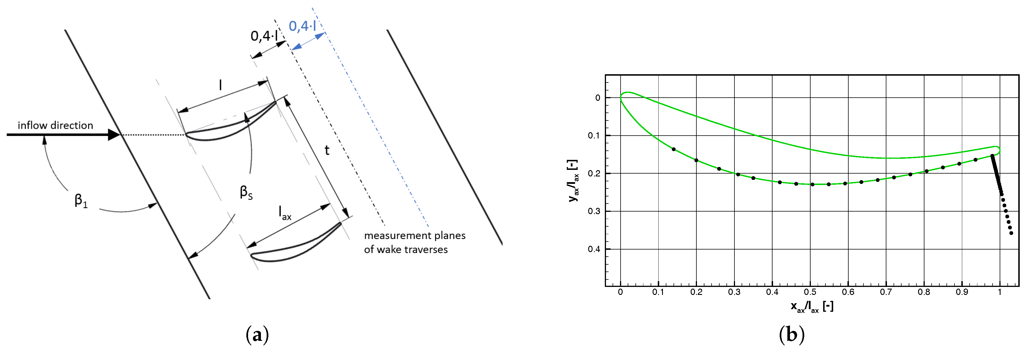
The wake traverses with the five hole probe at 40 % or 80 % of the chord length l behind the trailing edge of the middle blade are used to determine an integral pressure loss coefficient according to the method reported in Amecke [17] which calculates a mixed out state using the conservation of mass, momentum and energy. The integral total pressure loss coefficient is determined as:
ζ 1 = p t 1 p t 2 p t 1 p 1
In Equation (1) p t 1 is the total inlet pressure, p 1 the static inlet pressure and p t 2 the outlet pressure which is computed according to Amecke [17] with the five hole probe pressures. If experiments are conducted with active flow control by pulsed blowing, the definition has to be slightly changed to account for the energy addition by the fluidic oscillators. This can be done by computing a corrected total inlet pressure by using conservation of energy as shown by Ardey [18]:
p t 1 = m ˙ 1 , p a s · c p 1 · T t 1 · ( p t 1 ) 1 γ γ + m ˙ A F C · c p , A F C · T t , P l · ( p t , P l ) 1 γ γ m ˙ 1 , p a s · c p 1 · T t 1 + m ˙ A F C · c p , A F C · T t , P l γ 1 γ
The inlet mass flow per passage m ˙ 1 , p a s is calculated by subtracting the AFC mass flow of one blade from the outlet mass flow per passage which is gained from the measurements with the five hole probe as:
m ˙ 2 , p a s = ρ 2 · c 2 , a x · h · t .
The total plenum temperature T t , P l as well as the total plenum pressure p t , P l are the average values of all three plenums.
With the actuation mass flow corrected inlet total pressure p t 1 a corrected integral total pressure loss coefficient can be defined accordingly to the definition as:
ζ 1 = p t 1 p t 2 p t 1 p 1
In order to respect the proprietary nature of the experimental data, all total pressure losses are normalized with a reference integral total pressure loss ζ r e f . It is the total pressure loss in the aerodynamic design point of a state of the art TEC.

4.2. Determination of the Optimal Mass Flow Rate

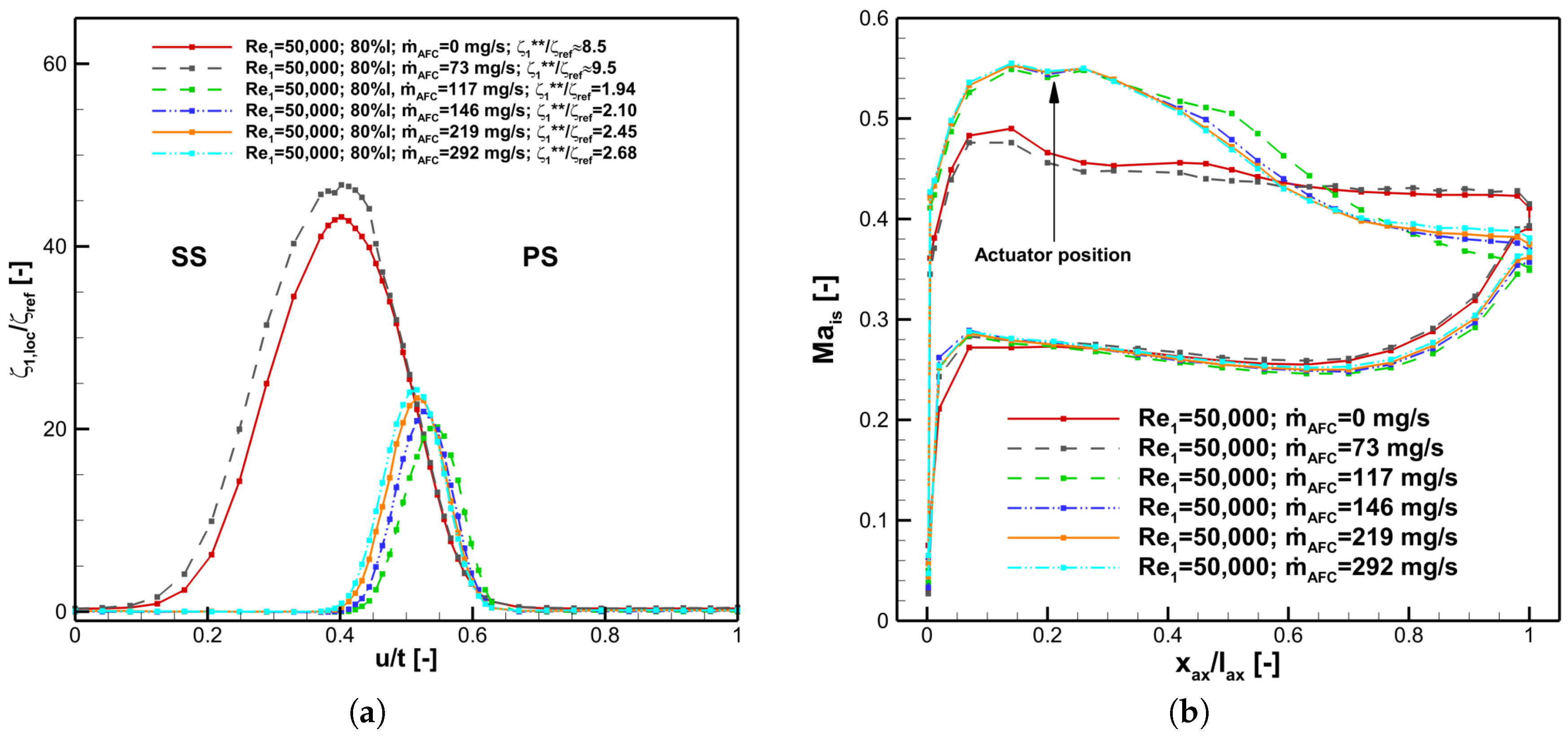
The optimal mass flow rate for each operating point was determined experimentally. Therefore, the resolution is limited as only discrete mass flow rates could be tested. Selection criterion for the optimal mass flow rate was the minimum corresponding total pressure loss. The effect of AFC on the total pressure losses and the profile Mach number distribution is exemplary shown for R e 1 = 50,000 in Figure 4.
Without actuation and with a mass flow rate of m ˙ A F C = 73 mg/s the Mach number distribution looks completely different than with higher mass flows. This indicates an open flow separation without reattachment. The impact on the whole flow behaviour around the profile is very strong as shown by Figure 4b. The peak Mach number on the suction side is considerably smaller and the Mach number at the trailing edge is much higher. That means the profile is not able to decelerate the flow as much as it was supposed to.
The referenced integral total pressure losses are also given in the left part of Figure 4. For this operating point a mass flow rate of m ˙ A F C = 117 mg/s is associated with the smallest total pressure losses. The corresponding mass flow ratio is m ˙ A F C / m ˙ 1 , p a s = 2.1 × 10 4 and the local pressure ratio is p t , P l / p l o c = 1.29 . Without active flow control, the losses are more than four times higher than in the case with optimal actuation mass flow. This is an impressive result and demonstrates the usefulness of the boundary layer control by this type of fluidic oscillator. As can be seen in Figure 4a at a mass flow rate of m ˙ A F C = 73 mg/s the measured total pressure losses are even higher than without actuation. Regarding the measured total pressure losses as a result of the profile boundary layer development, the increase in total pressure losses can be explained by a slightly thicker boundary layer on the suction side due to a negative effect of the additional mass flow from the actuator. However, this disturbance of the boundary layer by the actuators is not sufficient to initiate boundary layer transition and the associated reattachment of the flow on the suction side.
Increasing the mass flow rate above m ˙ A F C = 117 mg/s leads to higher total pressure losses. Yet, these losses are considerably lower than the losses of the two fully separated cases with and without m ˙ A F C = 73 mg/s mass flow rate. The data indicate that the optimal actuation flow rate is the smallest actuation flow rate which is able to initiate boundary layer transition and leads to reattachment of the flow on the suction side for operating points with small Reynolds numbers and open flow separation. For this profile, smaller losses can occur with a small separation bubble on the suction side compared to a case without separation bubble but earlier transition. By design intent, the displacement effect of the separation bubble can shift the diffusion of the flow towards the trailing edge. Ludewig et al. [19] also reported for steady blowing on a low pressure turbine profile that minimum total pressure losses occur with a small separation bubble on the suction side.
The profile Mach number distribution in the right part of Figure 4 shows that with the optimal mass flow rate of m ˙ A F C = 117 mg/s, the smallest Mach number at the trailing edge is measured. This is confirmed by the data from the wake traverse. For the optimal mass flow rate, the smallest outlet Mach number and the highest flow turning was computed with the measurement data in the outlet plane.

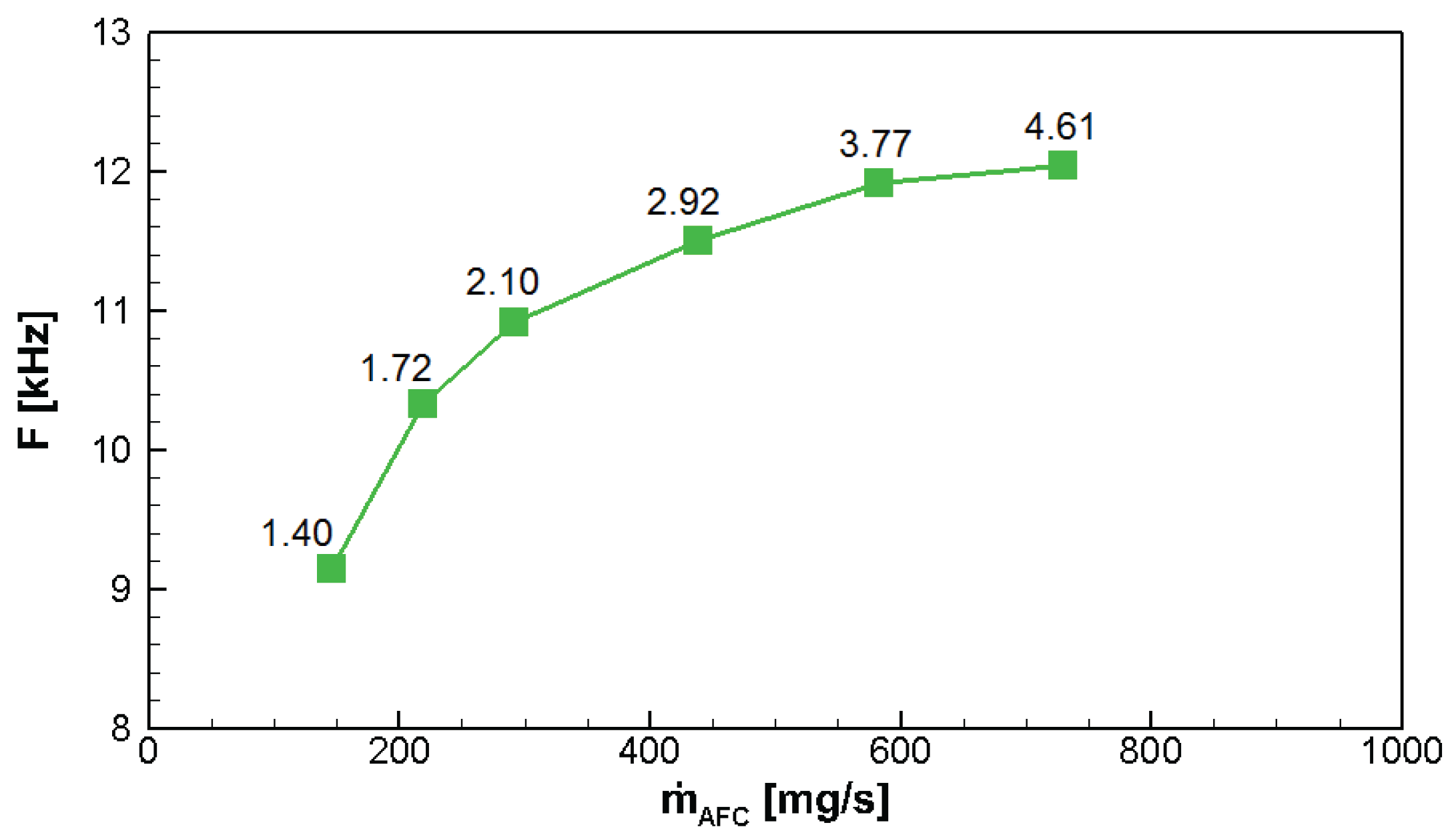
4.3. Actuation Frequency

In former publications e.g., by Mack et al. [10] it was also stated that the frequency of the oscillation plays a major role for the effectiveness of the actuation. Therefore, the frequencies belonging to the different mass flow rates were measured here with a single-sensor hot wire probe. The results from these measurements are presented in Figure 5 for R e 1 = 50,000. Furthermore, the corresponding pressure ratio p t , P l / p l o c of the oscillator is shown directly next to every data point in Figure 5.
The lowest frequency shown in Figure 5 was measured for a mass flow rate of 146 mg/s. For a mass flow rate of 73 mg/s no stable oscillation frequency could be detected. Unfortunately, no measurement data for the optimal mass flow rate of 117 mg/s is available yet, as the frequencies were measured before the optimal mass flow rate was determined.
Niehuis and Mack [4] reported that the amplification of Tollmien-Schlichting waves could be beneficial as this would accelerate the transition process. Therefore, a CFD study was conducted with MISES to determine the boundary layer data at the location of the fluidic actuators. More information on the CFD data and the utilized setup can be found in Kurz et al. [20]. With the numerical data, a stability analysis using the Orr-Sommerfeld equations as shown by Mack et al. [10] can be conducted. This leads to actuation frequencies at the blowing position between 15 kHz and 30 kHz with an optimum at approximately 24 kHz. These frequencies were not reached by the fluidic oscillators applied here. However, active flow control by these fluidic oscillators was successful as stated by the reduced total pressure losses. As reported by Kurz et al. [20], the most amplified instability frequencies according to linear stability theory decrease significantly towards the separation point. At the separation point of the operating conditions of R e 1 = 50,000, the optimal instability frequency was calculated as 7.9 kHz. As a consequence, the range of the amplified instability frequencies is met by the actuator close to the separation point, if the actuator frequencies are not completely damped by the main flow. Furthermore, the current experiments suggest that the actuation mass flow is an important criterion for effective flow control. Therefore, more experimental data with independent variation of mass flow and frequency is desirable and needed to determine more precise criteria for AFC concepts by pulsed blowing.

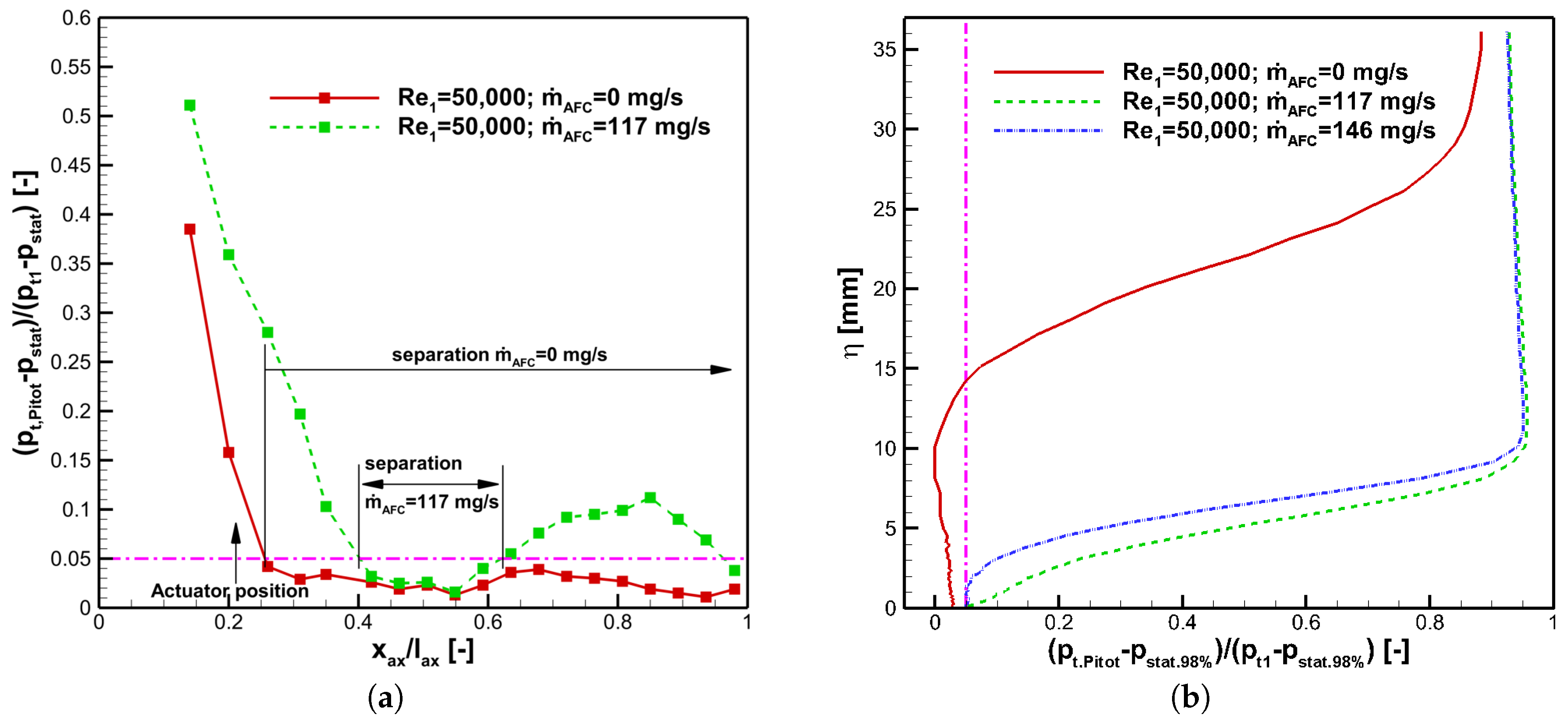
4.4. Boundary Layer Development on the Suction Surface

In order to gain more information on the influence of active flow control on the aerodynamics of the TEC-profile, measurements with a flattened Pitot probe were conducted. As the suction side aerodynamics are essential for the losses, the boundary layer measurements are constrained to the suction side of the profile.
In Figure 6 a dynamic pressure ratio according to the definition
q P i t o t q ( η , x a x / l a x ) = p t , P i t o t ( η , x a x / l a x ) p s t a t ( 0 , x a x / l a x ) p t 1 p s t a t ( 0 , x a x / l a x )
is shown. In Equation (5) p t , P i t o t ( η , x a x / l a x ) is defined as total pressure measured with the flattened Pitot probe at the position x a x / l a x with the distance η to the profile surface. The total inlet pressure p t 1 is measured at the same instant of time. The local surface pressure on the suction side p s t a t at the position x a x / l a x is measured with the static pressure taps, but with the flattened Pitot probe moved to a position where it does not affect the profile pressure distribution. During the measurements of the surface pressure ratio, the distance to the profile surface η is geometrically half of the probe head height of the flattened Pitot probe as the probe head is supposed to lie flat on the suction side surface: η = 0.15 mm.
For the measurement of the boundary layer with the flattened Pitot probe, the same dynamic pressure ratio is utilized. The static surface pressure p s t a t is in this case the static pressure at the position of the boundary layer traverse. This means it is the static surface pressure at x a x / l a x = 98 % .
In separation bubbles, the dynamic pressure ratio q P i t o t / q ought to be zero or at least close to zero as the reverse flow occurring in separation bubbles is not supposed to be measured by the flattened Pitot probe. Due to vortex structures in the bubble as well as the distance between the stream line through the Pitot probe head and the suction side surface, the actually measured dynamic pressure ratios are normally slightly bigger than zero especially when the separation bubbles are thin. This was also confirmed by Stotz et al. [14] who compared constant temperature anemometry (CTA) boundary layer measurements to this measurement technique. In the current measurements, due to the comparison with the Mach number distribution, a pressure ratio below q P i t o t / q = 0.05 is regarded as close enough to zero to represent a separation zone. The limit is shown in Figure 6a as a pink dash dot line.
The dynamic pressure ratios shown in Figure 6a start at x a x / l a x = 14 % which was the first static pressure tap that could be reached with the flattened Pitot probe. Without active flow control, the dynamic pressure ratio decreases from the first measurement position with a steep gradient. For a laminar boundary layer with a Blasius profile this means that the boundary layer thickness is increasing. The pressure ratio reaches a very small value below q P i t o t / q = 0.05 at x a x / l a x = 26 % and does not rise above this value for all following measurement points on the suction side. Hence, there is separation on the suction side which does not reattach before the trailing edge of the profile. This is also called an open flow separation on the suction side.
With active flow control at the optimal mass flow rate of m ˙ A F C = 117 mg/s the dynamic pressure ratio also decreases below the separation line at approximately at x a x / l a x = 40 % . However, a short separation region is followed by a rise of the dynamic pressure ratio above the separation line which is an indication for boundary layer transition from laminar to turbulent. Schlichting [21] stated by experiments on a flat plate without separation that due to the change in the boundary layer profile between a laminar and a turbulent boundary layer profile, a Pitot probe which is moved parallel to a wall with a fixed distance will measure a total pressure increase in the transition zone.
Using the pressure increase as selection criterion, the transition zone can be located in the region from about 55 % to 85 % of the axial chord length for the case with active flow control. Towards the trailing edge, the pressure ratio decreases. Thus, the boundary layer thickness is increasing towards the trailing edge. The last measurement point is even below the pressure ratio separation limit of q P i t o t / q = 0.05 which could be an indication for turbulent flow separation. However, the boundary layer profile measurements in Figure 6b for this mass flow rate show a pressure gradient directly at the suction surface which supports the assertion that the boundary layer is attached to the suction surface. In separated flows the pressure gradient measured with the flattened Pitot probe is supposed to be zero or close to zero as for example shown by the red curve without AFC in Figure 6b.
Comparing the boundary layer measurements perpendicular to the suction surface at 98 % of the axial chord length which are shown in the right part of Figure 6, there is a considerable difference between the cases with and without active flow control. Without active flow control the pressure ratio stays close to zero for approximately 10 mm perpendicular to the surface. From this it can be concluded that there is a thick layer on the suction side surface where no flow parallel to the profile suction surface in flow direction can be observed. This flow phenomenon is typical for separation bubbles. For both actuated cases the boundary layers are remarkably thinner. The optimal mass flow rate of m ˙ A F C = 117 mg/s has a slightly thinner boundary layer than the higher mass flow rate. This coincides with the total pressure losses which are also lowest for the mass flow rate of m ˙ A F C = 117 mg/s. As the boundary layer measurements and the wake traverses were all conducted at the same positions, the results can be directly compared to each other. For the cases without and with AFC an approximately three times higher boundary layer thickness on the suction side leads to an approximately two times wider wake (see Figure 4, left). The main difference of the wake can be localized on the suction side part of the wake. Regarding the boundary layer, development especially on the suction side of the profile as reported by Curtis et al. [1] as the main contributor to the total pressure losses represented by the wake, the results match very well.

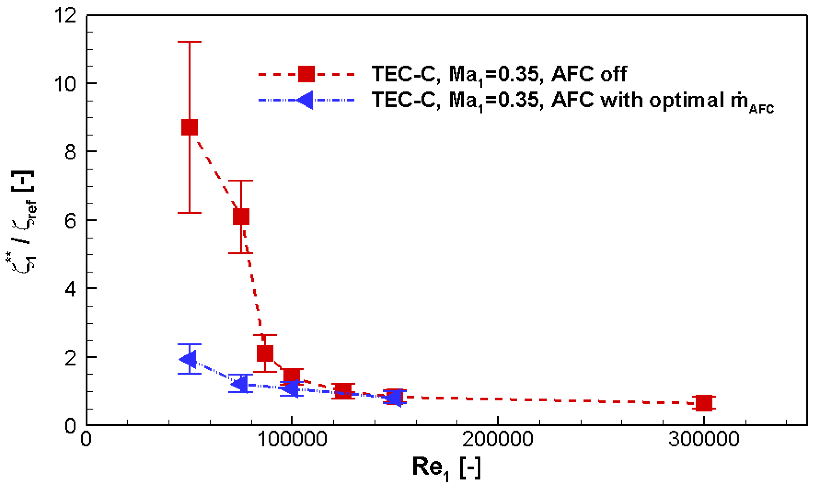
4.5. Reynolds Number Variation

After the detailed discussion of the benefit of active flow control in the low Reynolds number range, it is worth taking a look at the full operating range. Figure 7 shows the normalized and corrected integral total pressure loss as it is defined in Equation (4) for different Reynolds numbers.
The data which is labeled as “AFC off” was measured with the same measurement setup, but without actuation mass flow. The measurement data “AFC with optimal m ˙ A F C ” was gained as described before by using for each Reynolds number the data with the lowest integral total pressure losses which were tested in the current experiments. For R e 1 = 300,000 there is no measurement value as every mass flow rate which was tested produced higher total pressure losses than the case without active flow control.
The measurement data for the integral total pressure loss in Figure 7 show that losses can be reduced by active flow control over the major part of the operating range of the TEC profile. For the low Reynolds number range the loss reduction is very significant as open flow separation could be prevented successfully. Nevertheless, active flow control also reduces the integral total pressure losses when there are only small separation bubbles present on the suction side for Reynolds numbers above R e 1 87,000.

5. Conclusions

A highly loaded turbine exit case profile with active flow control by fluidic actuators was experimentally investigated in a high speed cascade wind tunnel with different measurement techniques. The concept of active flow control by fluidic oscillators is very successful as a substantial reduction of total pressure losses can be achieved for a Reynolds number of R e 1 = 50,000. This loss reduction can be gained by changing the flow behaviour on the suction side from open flow separation to a closed separation bubble. Due to this loss reduction, the safe and low loss operating range of the TEC profile with active flow control is significantly enlarged compared to the operating range of the same profile without active flow control.
Total pressure loss data show that active flow control is beneficial on the presented TEC airfoil for inflow Reynolds numbers up to R e 1 = 150,000. Only for the highest measured inlet Reynolds number R e 1 = 300,000 is it advantageous to switch-off the active flow control. Therefore, this flow concept was proven to be very successful over a broad operating range.
According to the stability analysis, the frequencies of the actuators were too small to ignite Tollmien-Schlichting waves at the blowing position, although the success of active flow control was proven by the current measurements. Towards the separation point, the most amplified instability frequencies are decreasing. As a consequence, the Tollmien-Schlichting frequencies can be met further downstream, if the actuator frequencies are not completely damped by the main flow. By downscaling the size of the actuator, the frequency of the oscillation could be increased, so that the Tollmien-Schlichting frequencies are met at the blowing position. Therefore, it would be of interest for following experiments to compare the performance of a smaller actuator with higher frequency and smaller mass flow rate to the measurement results with the present actuator.
Another topic for further investigation will be the influence of unsteady wakes on this type of highly loaded profile with active flow control. Howell et al. [22] reported that they can reduce the number of blades in a low pressure turbine by 15 % as the incoming wakes of upstream blade rows can have a beneficial effect on the boundary layer and therefore on the losses of the profile. That is why further measurements will be conducted with this TEC cascade using a wake generator with moving bars to simulate blade row interaction. The unsteady inflow conditions will probably have a beneficial effect on the separation bubble. Nevertheless, the high loss reductions for steady inflow conditions suggest that the usage of fluidic actuators will still be very valuable. Bons et al. [23] for example reported that the combination of unsteady wakes with flow control by vortex generator jets could reduce total pressure losses by 60 % compared to the case with unsteady wakes only.

Acknowledgments

The research leading to these results has received funding from the European Union Seventh Framework Programme (FP7) through the ENOVAL project under grant agreement No. 604999. The authors would like to thank the European Union for their support. Furthermore, the authors would like to thank the technical staff at Institute of Jet Propulsion for their great work in this project.

Author Contributions

The presented work is part of the research effort of Julia Kurz, who designed the TEC-C cascade, as well as planned and performed the measurement campaigns. In addition she analyzed the experimental data, performed the post processing including the programming of additional software tools and wrote the paper. Martin Hoeger supported the aero design of the new TEC-C profile with his broad experience in turbomachinery. As the head of the Institute of Jet Propulsion Reinhard Niehuis initiated the work, performed scientific supervision of all research activities and contributed to the writing of the paper.

Conflicts of Interest

The authors declare no conflict of interest. The founding sponsors had no role in the design of the study; in the collection, analyses, or interpretation of data; in the writing of the manuscript, and in the decision to publish the results.

Abbreviations

Abbreviations
AFCactive flow control
CFDcomputational fluid dynamics
FSfull scale
PSpressure side
Rdreading
SSsuction side
TECturbine exit case
Symbols
cvelocity
c p specific heat capacity
ddiameter
Ffrequency
hblade height
lchord length
m ˙ mass flow
M a Mach number
ppressure
qdynamic pressure
R e Reynolds number
tpitch
Ttemperature
T u free-stream turbulence level
upitchwise coordinate
xstreamwise coordinate
β angle
γ heat capacity ratio
ζ pressure loss coefficient
η distance normal to blade surface
ρ density
Subscripts
1inlet conditions
2outlet conditions
local free-stream condition
A F C active flow control
a x axial
i s isentropic
l o c local value
p a s middle flow passage
P i t o t measured with a Pitot probe
P l plenum
Sstagger
ttotal
Wwind tunnel coordinate system

References

  1. Curtis, E.M.; Hodson, H.P.; Banieghbal, M.R.; Denton, J.D.; Howell, R.J. Development of Blade Profiles for Low-Pressure Turbine Applications. J. Turbomach. 1997, 119, 531–538. [Google Scholar] [CrossRef]
  2. Kurz, J.; Niehuis, R.; Hoeger, M. Design of a Highly Loaded Turbine Exit Case Airfoil with Active Flow Control. In Proceedings of the ASME 2016 International Mechanical Engineering Congress and Exposition, Phoenix, AZ, USA, 11–17 November 2016. Paper No. IMECE2016-66008. [Google Scholar]
  3. Cattafesta, L.N.; Sheplak, M. Actuators for Active Flow Control. Annu. Rev. Fluid Mech. 2011, 43, 247–272. [Google Scholar] [CrossRef]
  4. Niehuis, R.; Mack, M. Active Boundary Layer Control with Fluidic Oscillators on Highly-Loaded Turbine Airfoils. In Active Flow and Combustion Control 2014; King, R., Ed.; Notes on Numerical Fluid Mechanics and Multidisciplinary Design Series 127; Springer International Publishing: Cham, Switzerland, 2014; pp. 3–22. [Google Scholar]
  5. Volino, R.J. Passive Flow Control on Low-Pressure Turbine Airfoils. J. Turbomach. 2003, 125, 754–764. [Google Scholar] [CrossRef]
  6. Bons, J.P.; Reimann, D.; Bloxham, M. Separated Flow Transition on an LP Turbine Blade With Pulsed Flow Control. J. Turbomach. 2008, 130, 021014. [Google Scholar] [CrossRef]
  7. Cerretelli, C.; Kirtley, K. Boundary Layer Separation Control With Fluidic Oscillators. J. Turbomach. 2009, 131, 041001. [Google Scholar] [CrossRef]
  8. Glezer, A.; Amitay, M.; Honohan, A.M. Aspects of Low- and High-Frequency Actuation for Aerodynamic Flow Control. AIAA J. 2005, 43, 1501–1511. [Google Scholar] [CrossRef]
  9. Wazzan, A.R.; Okamura, T.T.; Smith, A.M.O. Spatial and Temporal Stability Charts for the Falkner-Skan Boundary-Layer Profiles; Report No. DAC-67086; Douglas Aircraft Company: Long Beach, CA, USA, 1968. [Google Scholar]
  10. Mack, M.; Niehuis, R.; Fiala, A. Parametric Study of Fluidic Oscillators for Use in Active Boundary Layer Control. In Proceedings of the ASME 2011 Turbo Expo: Turbine Technical Conference and Exposition, Vancouver, BC, USA, 6–10 June 2011. Paper No. GT2011-45073. [Google Scholar]
  11. Bons, J.P.; Sondergaard, R.; Rivir, R.B. The Fluid Dynamics of LPT Blade Separation Control Using Pulsed Jets. J. Turbomach. 2001, 124, 77–85. [Google Scholar] [CrossRef]
  12. Sturm, W.; Fottner, L. The High-Speed Cascade Wind Tunnel of the German Armed Forces University Munich. In Proceedings of the 8th Symposium on Measuring Techniques for Transonic and Supersonic Flows in Cascades and Turbomachines, Genoa, Italy, 24–25 October 1985. [Google Scholar]
  13. Yang, S.L.; Spedding, G.R. Passive separation control by acoustic resonance. Exp. Fluids 2013, 54, 1603. [Google Scholar] [CrossRef]
  14. Stotz, S.; Wakelam, C.T.; Niehuis, R. Investigation of the Suction Side Boundary Layer Development on Low Pressure Turbine Airfoils With and Without Separation Using a Preston Probe. In Proceedings of the ASME Turbo Expo 2014: Turbine Technical Conference and Exposition, Düsseldorf, Germany, 16–20 June 2014. Paper No. GT2014-25908. [Google Scholar]
  15. Brachmanski, R.; Niehuis, R.; Bosco, A. Investigation of a Separated Boundary Layer and Its Influence on Secondary Flow of a Transonic Turbine Profile. In Proceedings of the ASME Turbo Expo 2014: Turbine Technical Conference and Exposition, Düsseldorf, Germany, 16–20 June 2014. Paper No. GT2014-25890. [Google Scholar]
  16. Tropea, C.; Yarin, A.L.; Foss, J.F. Springer Handbook of Experimental Fluid Mechanics; Springer: Berlin/Heidelberg, Germany, 2007. [Google Scholar]
  17. Amecke, J. Auswertung von Nachlaufmessungen an Ebenen Schaufelgittern; Report 67 A 49; AVA: Goettingen, Germany, 1967. [Google Scholar]
  18. Ardey, S. Untersuchung der Aerodynamischen Effekte von Vorderkanten-Kühlluftausblasung an Einem Hochbelasteten Turbinengitter. Ph.D. Thesis, Universität der Bundeswehr München, Neubiberg, Germany, 1998. [Google Scholar]
  19. Ludewig, T.; Mack, M.; Niehuis, R.; Franke, M. Optimization of the Blowing Ratio for a Low Pressure Turbine Cascade with Active Flow Control. In Proceedings of the 9th European Conference on Turbomachinery (ETC), Istanbul, Turkey, 21–25 March 2011. Paper No. 131. [Google Scholar]
  20. Kurz, J.; Hoeger, M.; Niehuis, R. Influence of Active Flow Control on different kinds of Separation Bubbles. In Proceedings of the 23rd International Symposium on Air Breathing Engines, Manchester, UK, 3–8 September 2017. Paper No. ISABE-2017-22572. [Google Scholar]
  21. Schlichting, H. Boundary-Layer Theory, 7th ed.; McGraw-Hill: New York, NY, USA, 1979. [Google Scholar]
  22. Howell, R.J.; Ramesh, O.N.; Hodson, H.P.; Harvey, N.W.; Schulte, V. High Lift and Aft-Loaded Profiles for Low-Pressure Turbines. J. Turbomach. 2001, 123, 181–188. [Google Scholar] [CrossRef]
  23. Bons, J.P.; Pluim, J.; Gompertz, K.; Bloxham, M.; Clark, J.P. The Application of Flow Control to an Aft-Loaded Low Pressure Turbine Cascade With Unsteady Wakes. J. Turbomach. 2011, 134, 031009. [Google Scholar] [CrossRef]
Figure 1. High Speed Cascade Wind Tunnel.
Ijtpp 03 00008 g001
Figure 2. Fluidic oscillators (a) geometrical dimensions and (b) their integration into the TEC blade.
Ijtpp 03 00008 g002
Figure 3. (a) Illustration of wake traverse measurement planes and (b) measurement positions of the flattened Pitot probe.
Ijtpp 03 00008 g003
Figure 4. (a) Local total pressure loss and (b) isentropic Mach number distribution for different mass flow rates at R e 1 =50,000.
Ijtpp 03 00008 g004
Figure 5. Actuation frequency over mass flow rate for R e 1 = 50,000.
Ijtpp 03 00008 g005
Figure 6. Dynamic pressure ratio (a) on the suction side surface and (b) as boundary layer profiles at 98 % of the axial chord length l a x for different mass flow rates at R e 1 = 50,000.
Ijtpp 03 00008 g006
Figure 7. Mass flow corrected integral total pressure loss for different Reynolds numbers.
Ijtpp 03 00008 g007
Table 1. Geometry and operating conditions of the TEC-C cascade.
DimensionSymbolValue
inlet Mach number M a 1 0.35
inlet flow angle β 1 118.2
inlet Turbulence intensity T u 1 1.9%
axial chord length l a x 66.6 mm
pitch to chord ratio t / l 1.44
stagger angle β S 81.6

