Article

A POD-Based Procedure for the Split of Unsteady Losses of an LPT Cascade †

1
DIME—University of Genoa, Via Montallegro 1, I-16145 Genoa, Italy
2
GE AvioAero SRL, Torino I-10040, Italy
*
Author to whom correspondence should be addressed.
This paper is an extended version of our paper in Proceedings of the European Turbomachinery Conference ETC12, 2017, Paper No. 324.
Int. J. Turbomach. Propuls. Power 2017, 2(4), 17; https://doi.org/10.3390/ijtpp2040017
Submission received: 6 June 2017 / Revised: 28 September 2017 / Accepted: 4 October 2017 / Published: 16 October 2017

Abstract

:
A time-resolved particle image velocimetry (TR-PIV) system has been employed to investigate the unsteady propagation of upstream wakes in a low-pressure turbine cascade. Data are obtained in the steady state condition and for two passing wake reduced frequencies. The study is focused on the identification and split of the different dynamics responsible for deterministic and random oscillations, thus loss generation by means of a new procedure based on proper orthogonal decomposition (POD). The paper takes advantage of the properties of POD that reduce the data set to a low number of modes that represent the most energetic dynamics of the system. It is clearly shown that the phase averaged flow field can be represented by a few number of POD modes related to the wake passing event for the unsteady cases. Proper orthogonal decomposition is also able to capture flow features affecting the instantaneous flow field not directly related to the wake passage (i.e., the vortex shedding phenomenon induced by the intermittent separation developing between adjacent wakes), which are smeared out in the phase averaged results. A procedure exploiting the biorthogonality condition of the POD modes, and the related temporal coefficients, has been developed for the quantification of the contribution due to the different POD modes to the overall turbulence kinetic energy production, or, equivalently, the mean flow energy dissipation rate. Results into the paper clearly show that losses due to wake migration, boundary layer and vortex shedding related phenomena can be distinguished and separately quantified for the different tested conditions.

1. Introduction

The deep understanding of the unsteady flow in turbomachines is a complicated task due to the superposition of different sources of unsteadiness. The blade boundary layer transition process due to a by-pass or separated like mechanisms, the von Karman vortex formation and incoming wake related events represent the common sources driving flow oscillations in the unsteady operation, thus the mechanisms responsible for loss generation [1]. Literature of the last 20 years clearly highlights that in low pressure turbine (LPT) rows the incoming passing wakes generate a jet-like structure that, impinging on the blade suction side, opens in two branches, generating two large scale coherent structures (e.g., [2,3,4]). The turbulence activity carried by these large scale vortices increases during migration across the downstream LPT passage, being the wake region stretched and bowed by the cascade pressure field. This process produces losses in the potential flow region due to the strong deformation of the wake apex [5], and also sensibly affects the near wall flow region. Indeed, the interaction between the turbulence carried by wakes and the suction side boundary layer is responsible for a bypass-like transition process. In this case, a dense population of streaky structures has been observed in the footprint of the region perturbed by wakes [6,7,8,9]. In this respect, the anticipation of the boundary layer transition contributes to delay or suppress the separation process that may occur on high lift profiles operating at low Reynolds number condition. All of these unsteady phenomena contribute to the overall amount of losses, and can present different sensitivity to variation of operating parameters characterizing the real operation of an LPT stage (i.e., Reynolds number, reduced frequency, incidence angle, etc.).
The recognition and/or the prediction of the aforementioned unsteady processes demands time-resolved techniques, either numerical or experimental. Detailed Unsteady Reynolds-Averaged Navier-Stokes (URANS) calculations are able to describe the evolution of the periodic part of the unsteady motion, but provide only the statistical evolution of the turbulent activity (e.g., [10]). Similarly, the phase-averaged treatment of experimental data allows the detailed analysis of the periodic flow due to the wake, while the random part of flow oscillations can be only statistically described [11]. In both cases, all the unsteadiness sources not directly related to the wake passing frequency are not resolved, and their role in the loss generation mechanisms remains substantially obscure. Much more complicated and time-consuming computations, like Large Eddy Simulation (LES) or Direct Numerical Simulation (DNS) are requested for this topic, even though their application in the design phase is still far from being possible.
The proper orthogonal decomposition (POD) is nowadays a well established mathematical procedure that has been largely used for the detection of coherent structures embedded within the flows (see, for example [12,13]), and recently has also been applied to obtain phase-averaged velocity fields (e.g., [14,15,16]). In the present paper, time-resolved particle image velocimetry (TR-PIV) measurements describing the flow field in a highly loaded LPT cascade have been analyzed with the aim of identifying, splitting and characterizing the different phenomena producing losses. To this end, POD has been applied to the instantaneous flow fields characterizing the steady state, and two different incoming wake reduced frequencies. For the steady case, POD has been proved to be able to identify structures associated with a by-pass-like transition process [17] as well as with the coherent structures shed as a consequence of the boundary layer separation [18,19]. On the other hand, in the unsteady case, the most energetic POD modes well describe the spatial structure of the negative jet and the related large scale vortices attached to the leading and trailing boundary of the wake (see [8,20]). In the present work, POD mode distributions and related temporal coefficients are first compared with time resolved and phase-averaged velocity fields in order to provide clear evidence of the physical meaning of each mode, and the flow dynamics it represents. The effects of the reduced frequency variation (from the steady state to the nominal unsteady condition) on the main dynamics inducing flow oscillations (i.e., boundary layer separation and incoming wake effects) will be deeply characterized by means of POD modes and related temporal coefficients. Additionally, making use of the biorthonormality of POD modes and the corresponding temporal coefficients, the contribution of each mode to both the normal and the shear Reynolds stresses is identified. The combination of the Reynolds stresses and the local flow distortion allows the computation of the TKE production rate or, equivalently, the loss generation rate per mode. This allows the identification and split of the role played by the different superposed phenomena on the overall amount of losses generation during the unsteady operation of an LPT cascade. The possibility to separate the loss contribution due to the different dynamics can provide a useful tool to establish or verify optimization criteria, thus contributing to the development of high efficiency new generation turbine stages.

2. Experimental Apparatus and Data Reduction

2.1. Test Facility and Instrumentation

The experimental investigations have been performed in the blow-down wind tunnel installed at the Aerodynamics and Turbomachinery Laboratory of the University of Genoa. The test section consists of a seven-blade large scale planar cascade (Figure 1), representative of highly loaded LPT blade profiles. Blades are characterized by a chord length of 120 mm, a pitch-to-chord ratio of 0.67, and an aspect ratio A R = 2.5 to ensure two-dimensional (2D) time–mean flow at midspan. This condition is necessary to compute all the TKE production terms with a 2D measurement system. The inlet flow angle is 40 º , and the blade turning around 100 º . Measurements have been carried out at a low Reynolds number condition R e = 70 , 000 with both steady and unsteady incoming flow. The inlet free-stream turbulence was T u = 4.2 % , with an integral length scale of around 15 mm.
Upstream wakes have been simulated by means of a tangential wheel of radial rods installed 1/3 of the axial chord upstream of the cascade leading edge plane. The flow coefficient was set to φ = 0.675 to be representative of real engine operative conditions. Two different reduced frequencies have been analyzed ( f + = 0.69 and f + = 0.35 ) referred to in the following as nominal and halved condition, respectively. The bar diameter (3 mm) was chosen so that the wake shed from the bars produce losses and shedding frequencies that are representative of those generated by a typical upstream LPT row. At the cascade entrance plane, the bar wakes are characterized by a pitch-wise extension of around 1/3 of the bars spacing, a maximum relative velocity defect of 15% and a turbulence intensity peak of around 30%. Details on the incoming wake structure and the facility are provided in Simoni et al. [21].
The blade aerodynamic loading has been surveyed on the three central blades in order to set the periodicity condition by means of adjustable tailboards and sidewall inlet bleeds. To this aim, each blade was instrumented at midspan with a total of 22 pressure taps connected to a Scanivalve (Scanivale Corporation, Liberty Lake, WA, USA). The maximum deviation between the loading distributions of the three blades was 2%.
Particle image velocimetry measurements have been performed in order to characterize the unsteady transition process of the suction side boundary layer perturbed by upstream wakes. The PIV field of view covers the flow region 0.55 < s / s m a x < 1.1 and 0.0 < y / g < 0.15 . A sketch of the measuring domain with respect to the blade surface is provided in the zoomed insert of Figure 1. Behind the blade trailing edge, a small flow portion into the wake region has been masked due to reflection (the dashed grey region). Similarly, due to wall reflection along the blade, a masked area (sketched in black in the figure) has been adopted to remove the first five pixels close to the wall. About 9000 couples of images have been acquired in order to obtain high statistical accuracy. A further data set of around 2000 images has been acquired in the unsteady cases at a lower acquisition frequency and with a larger extension in the pitchwise direction ( 0.0 < y / g < 0.46 ) for a better characterization of the wake migration process in the potential flow region.
The light source is a dual-cavity Nd:YLF pulsed laser Litron LDY (Rugby, UK) 300 (energy 30 mJ per pulse at 1000 Hz repetition rate, 527 nm wavelength). The optical system forms a light sheet of 1 mm thickness. The light scattered by the seeding particles (vaseline oil droplets with a mean diameter of 1.5 μ m) is recorded on a high sensitive SpeedSense M340 digital camera (Vision Research, Inc., Wayne, NJ, USA) with a cooled 2560 × 1600 pixels CMOS matrix. The camera frame rate has been set to 2000 Hz reducing the field of view of the camera to 2560 × 400 pixels and operating it in double frame mode. The magnification factor for the present experiments was set to 0.285 in order to obtain a high spatial resolution. This provides a particle image diameter on the order of 2–3 pixels and a pixel concentration of around four particles per investigation area. The Dantec Dynamics Studio tool (v. 4.15.115, Dantec Dynamics, Skovlunde, Denmark) has been used for the cross-correlation of each image pair. The adaptive cross-correlation algorithm has been used with a finer interrogation area of 16 × 16 pixels, and 50% overlap. This gives a distance between adjacent vectors of 0.28 mm. This spatial resolution allows for observing the boundary layer with at least 15 measuring points, and to consequently solve with great detail the large scale structures that characterize the transitional boundary layer that are responsible for the largest quota of the TKE production rate. However, it is worth noting that the first measuring point is too far from the wall to collect data into the viscous sublayer. A peak validation has been used to discriminate between valid and invalid vectors. With these settings, a Gaussian fitting procedure is likely to guarantee a sub-pixel recognition accuracy of particle displacement of the order of 0.1 pixels, in accordance with the accuracy analysis reported in Sciacchitano et al. [22] and Wieneke [23]. Limiting the maximum particle displacement to 1/4 of the investigation area, the relative error in the evaluation of the instantaneous velocities is less than ± 3.0%.

2.2. Data Analysis

The TR-PIV data have been analyzed by means of POD in order to highlight the dynamics related to the different sources of unsteadiness, thus providing new insight into the mechanisms producing losses in the unsteady operation of the LPT cascade. The POD is performed in the present work following the mathematical procedure described in Sirovich [24]. According to this procedure, given N statistical independent realizations (N PIV instantaneous flow fields), the POD is reduced in finding the eigenvalues Λ and the eigenvectors X of a cross-correlation matrix C [ N × N ]. The i , j element of the matrix C is defined as the surface integral of the velocity fields at times i and j. The POD modes are finally obtained projecting the original data on the computed eigenvectors.
These operations can be conveniently expressed and performed in matrix form, since the collected data are discrete in space and time.
M = u x 1 , y 1 ( 1 ) u x 2 , y 1 ( 1 ) u x L , y 1 ( 1 ) u x 1 , y 2 ( 1 ) u x L , y L ( 1 ) v x 1 , y 1 ( 1 ) v x L , y L ( 1 ) u x 1 , y 1 ( 2 ) u x L , y L ( 2 ) v x 1 , y 1 ( 2 ) v x L , y L ( 2 ) . . u x 1 , y 1 ( N ) u x L , y 1 ( N ) u x L , y L ( N ) v x 1 , y 1 ( N ) v x L , y L ( N )
where the apex (*) indicates the image number and the terms x L , y L are the number of measurement points along the x and y direction, respectively. Thus, each line of M has the length of 2 × x L × y L . According to this definition of the matrix M, the cross correlation matrix C is obtained as:
C = 1 N MM T .
The eigenvalues Λ and the eigenvectors X of the cross-correlation matrix C are obtained solving the eigenvalue problem:
CX = Λ X .
Since C is a symmetric square matrix of size [ N × N ], the eigenvalues of C are then real and non-negative and the eigenvectors are orthonormal. The POD modes are computed by projection as:
Φ = M T X .
This procedure provides a triplet of information: the eigenvalues λ ( k ) , the eigenvectors χ ( k ) and the POD modes ϕ ( k ) . The eigenvalue of the k t h mode represents the energy contribution of the mode to the total kinetic energy of velocity fluctuations. The eigenvectors constitute an orthogonal basis and retain the temporal information related to each mode. They can be used to provide phase averaged flow field without using an external trigger signal as discussed in Lengani et al. [18], as well as to analyze the characteristic frequency of each structure. The POD modes constitute an orthogonal basis that provides the spatial information identifying coherent structures in the flow. Note that, during projection of the elements of the data matrix on the eigenvectors (Equation (4)), both streamwise and wall normal velocity components POD modes can be identified ( ϕ i in the following equation) considering only the projection of the related velocity. Since the POD modes and eigenvectors are orthogonal, the Reynolds shear and normal stresses can be computed, adopting an index notation, as:
u i u j ¯ = k λ ( k ) ϕ i ( k ) ϕ j ( k )
The term λ ( k ) ϕ i ( k ) ϕ j ( k ) represents the contribution of the k t h POD mode to the overall time-mean Reynolds stresses. This property of POD can be applied to split the contribution to the TKE production terms P T K E . For 2D time-mean flows, in Cartesian notation P T K E assumes the form:
P T K E = u 2 ¯ u ¯ x u v ¯ u ¯ y u v ¯ v ¯ x v 2 ¯ v ¯ y .
P T K E also represents the mean flow loss generation rate, since it appears in both the TKE and mean flow kinetic energy transport equations but with a reversed sign. Each term appearing in Equation (6) can be generically represented as:
p i j = u i u j ¯ u ¯ i x j .
Substituting Equation (5) in Equation (7), the contribution of each POD mode to the production rate of each term p i j can be computed as:
p i j ( k ) = λ ( k ) ϕ i ( k ) ϕ j ( k ) u ¯ i x j , w i t h p i j = k p i j ( k )
According to these equations, each POD mode contributes to a quota of the time-mean TKE generation rate, explicitly appearing in Reynolds averaged formulation of the Navier–Stokes equations. Therefore, the contributions to the overall losses due to boundary layer, wake migration and their combination can be split and analyzed separately, thus providing further insight into the mechanisms producing losses. The largest error in the determination of the TKE production is due to the computation of the time mean velocity gradient while the statistical error in the computation of the Reynolds shear stress per POD mode is very small since the database is constituted by 9000 data and, in the worst condition, at least 90 wake passing periods have been surveyed with 100 snapshots per period. Typically, POD reaches a statistical convergence at the first 10 modes for more than 200 data (e.g., see Lacarelle et al. [25]).

3. Results and Discussion

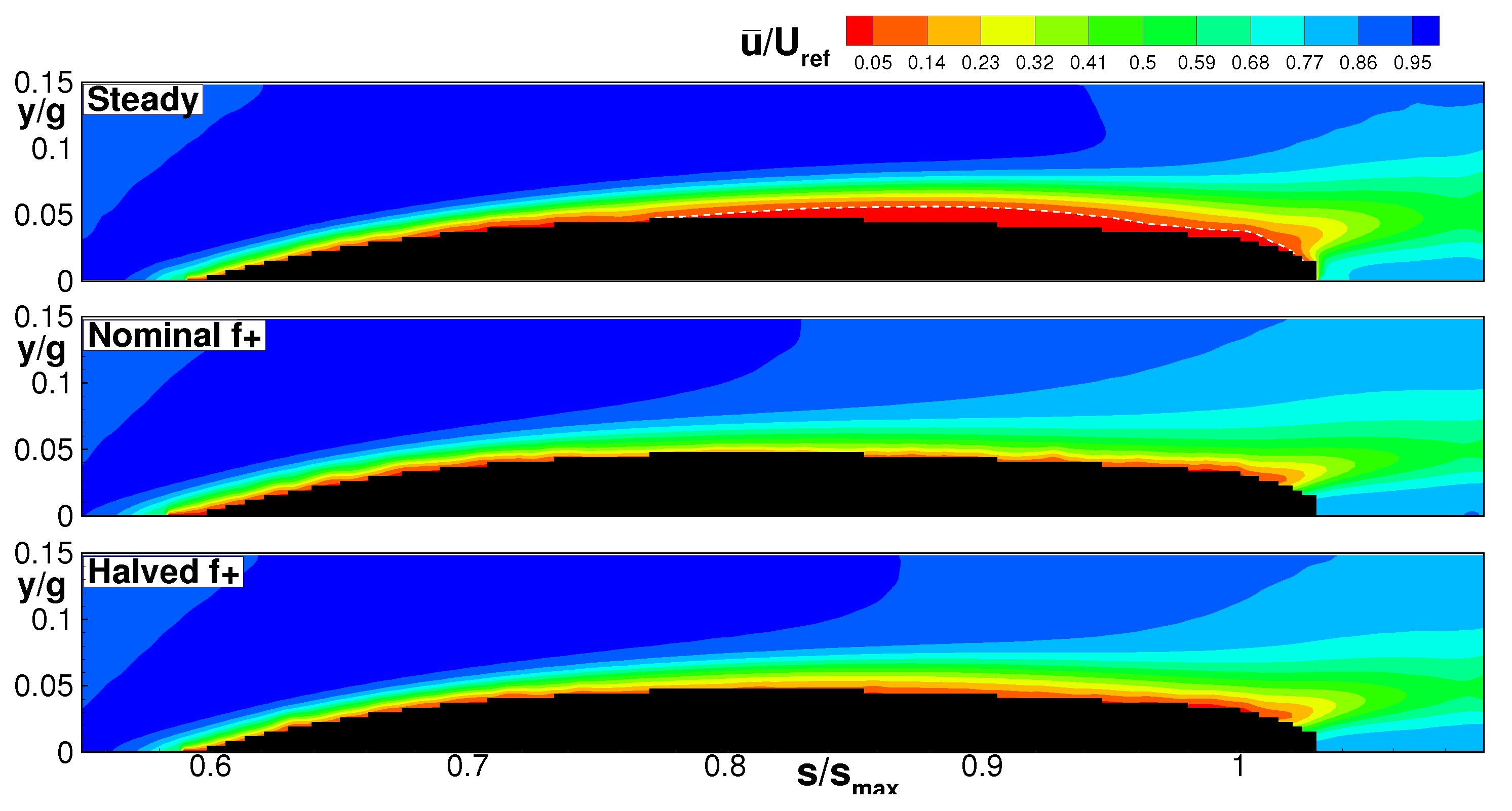
The time-mean velocity distributions of the steady state and the two unsteady cases are represented in Figure 2. The steady state condition shows a separated boundary layer with zero velocity in the aft portion of the blade suction side. The bubble maximum displacement position is located at around s / s m a x = 0.9 , and the boundary layer does not reattach prior to the trailing edge. Conversely, due to the wake effects, the boundary layer appears completely attached in the nominal unsteady case. These results confirm the well-known beneficial effects of unsteady passing wake in suppressing separation (e.g., [3,26]). Time-mean boundary layer separation seems to not be present either for the f + = 0.35 condition, even though lower velocity levels can be observed close to the wall, midway between the two previous conditions, as expected. As it will be discussed in the following, this latter condition is characterized by an unsteady separation, and POD will be shown to clearly capture the dominant dynamics responsible for flow oscillations and losses in the different conditions.

3.1. Unsteady Flow Analysis

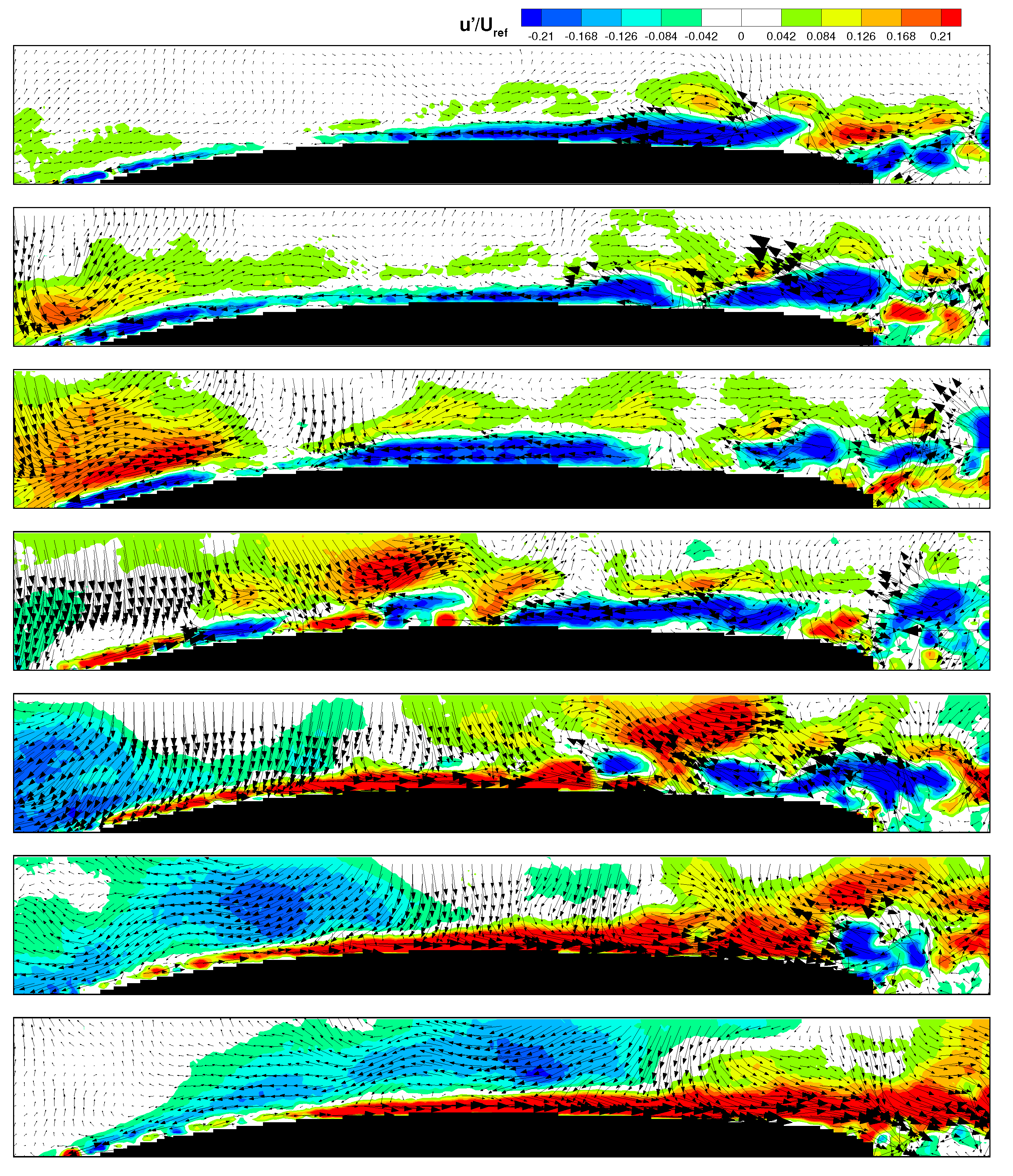
Thanks to the high frequency response of the TR-PIV instrumentation, the evolution of the flow field can be directly observed to provide a clear view of the flow unsteadiness and complexity. In Figure 3, evenly time spaced instantaneous perturbation velocity vector maps, ( u , v ) according to the Reynolds decomposition, are reported for the case f + = 0.35 . The color plots of u are also superposed to empathize the occurrence of localized low and high speed velocity regions during the wake-boundary layer interaction process. About half of the blade passing period is considered. In the first frame the boundary layer develops unperturbed by the wakes. Large negative values of u can be observed in the aft portion of the blade suction side, jointly with the occurrence of large scale vortical structures. Due to the low reduced frequency unsteady boundary layer separation occurs between adjacent wakes, similarly to the results of Opoka and Hodson [27]. The wake is entering the domain at the second time instant, as it can be deduced by the positive values of u in the fore portion of the suction side away from the wall. While the wake is moving along the fore part of the blade (see the second and third images) the separated flow region in the rear part of the blade still sheds vortices. As soon as the wake interacts with the near wall low velocity region, roll up vortices originate as a consequence of the high shear effects induced by the leading boundary of the wake patch (see the vector maps in the neighboring of the blue area in the fore portion of the blade in the fourth frames). Later, the wake moves further downstream and starts interacting with the separated flow region, and the unsteady behavior of the near wall flow becomes extremely complex. Separation is fully suppressed in the sixth and seventh images, where the region close to the wall is characterized by large positive values of u . In the last frame, the flow appears quite ordered even thought the wake is still interacting with the boundary layer, as highlighted by the elevated negative u values outside the boundary layer region. Wake boundary layer interaction manifests low random oscillations at the end of the interaction process, since the turbulent activity carried by the wake is mainly concentrated at its leading boundary, as described in Lengani et al. [8].
The unsteady flow field observed here is clearly characterized by stochastic and deterministic (periodic) events due to roll up vortices and wake related effects, respectively. Deterministic fluctuations are classically analyzed by means of phase averaged data, which are able to solve the periodic motion but provide only a statistical representation of the stochastic activities (through the phase-locked root mean square (rms) distribution). On the other hand, POD can be used to characterize the spatio-temporal evolution of both deterministic and stochastic phenomena that contribute to the unsteady flow field just observed, as discussed in previous publications [8,17].
The ability of POD of resolving deterministic events can be appreciated by the comparison between the most energetic POD modes and the phase-averaged flow field. In Figure 4 and Figure 5, results for the nominal f + case are reported as examples.
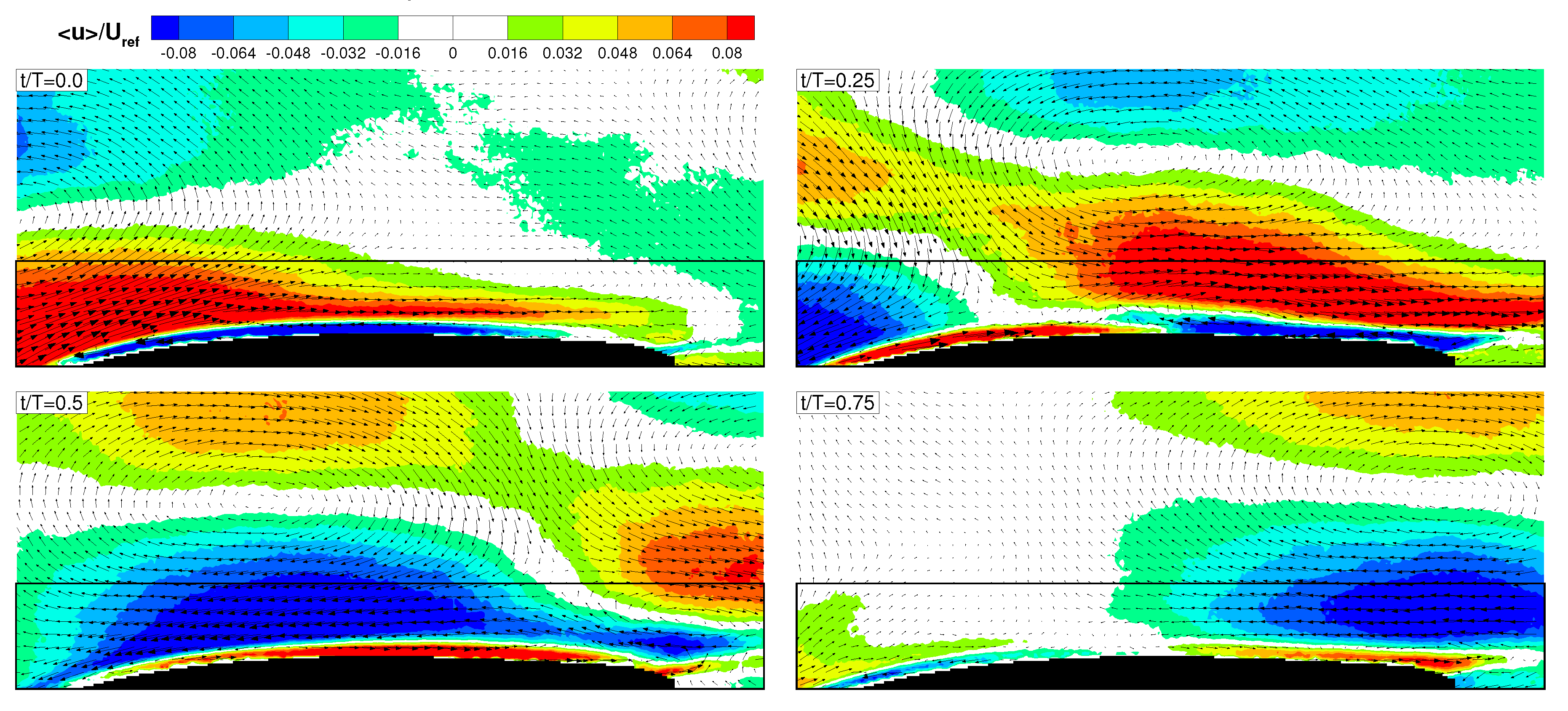
Figure 4 shows the phase-averaged flow evolution for different phases. The contour plot of the purely periodic component ( < u ( t / T ) > = u ˜ ( t / T ) u ¯ , where u ˜ ( t / T ) is the phase averaged velocity) and the vectorial representation of < u > , < v > are represented in the pictures. The reconstructed phase-averaged velocity field is represented as a plot sequence for four phases within a wake passing period. The extended measurement domain is considered in this case to better appreciate the large scale structures induced by the wakes.
The first instant ( t / T = 0.0 ) captures the wake entering the measurement domain, since a large scale counter-clockwise rotating vortex is clearly observable in the fore portion of the measuring domain. As described in Gompertz and Bons [2], it is due to the low momentum wake flow that impinges on the blade surface opening in two branches. The stream at the leading boundary of the wake induces positive values of < u > at the edge of the boundary layer, thus provoking high shear effects and the formation of roll up vortices, as previously observed in the instantaneous images. However, since these vortices are not locked to the passing wake, they are smeared out by the phase-averaging procedure and cannot be consequently observed in Figure 4. The wake jet structure pointing toward the wall can be clearly recognized at t / T = 0.25 , while the clockwise rotating structure successively appears as the wake moves further downstream (at t / T = 0.5 and t / T = 0.75 ).
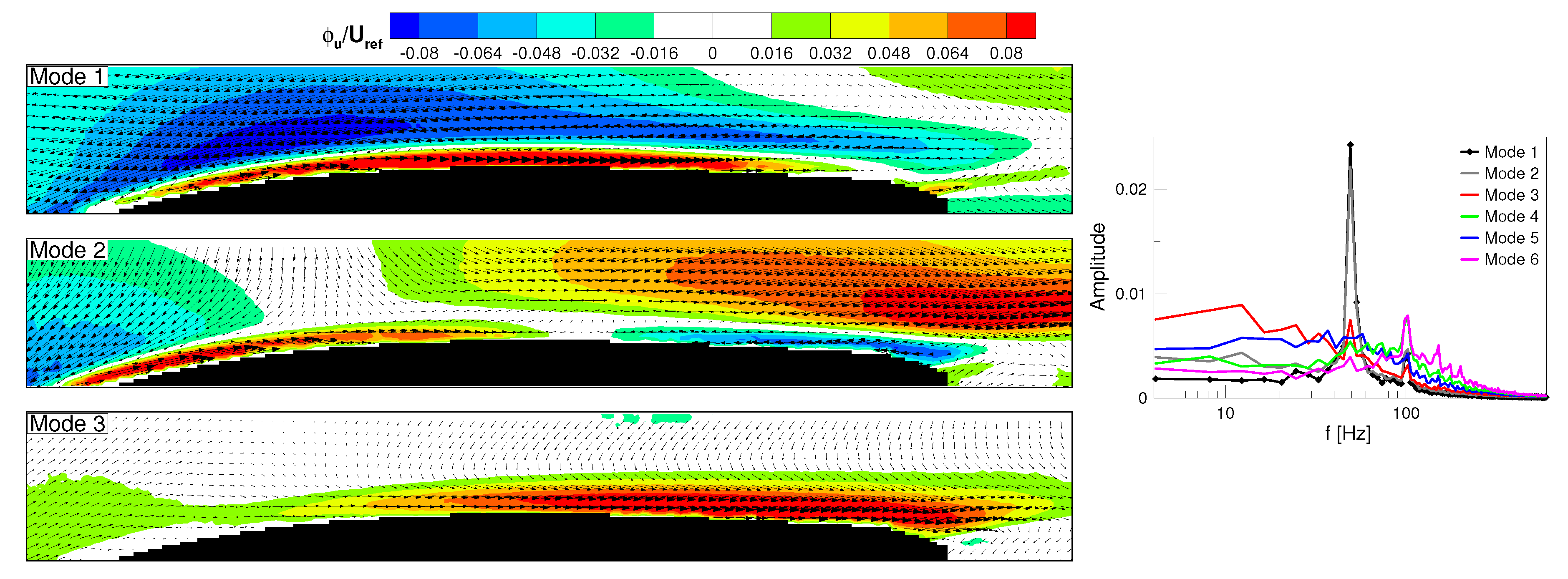
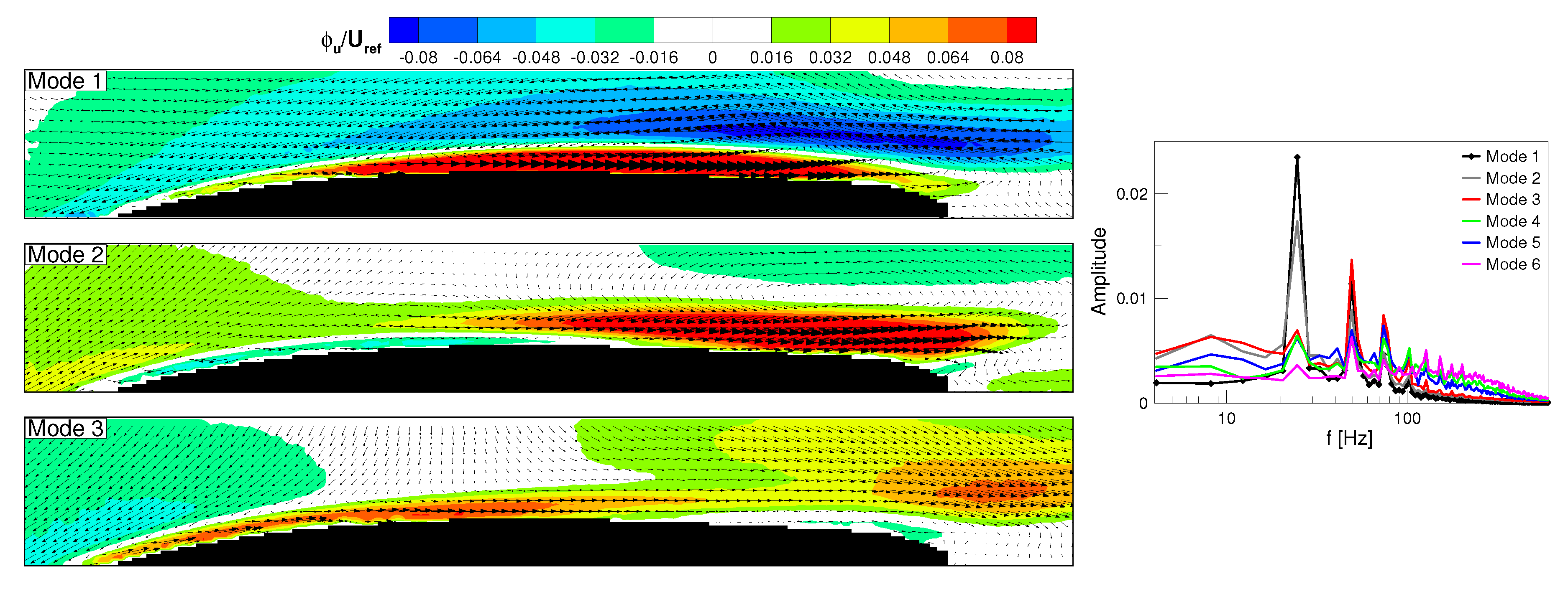
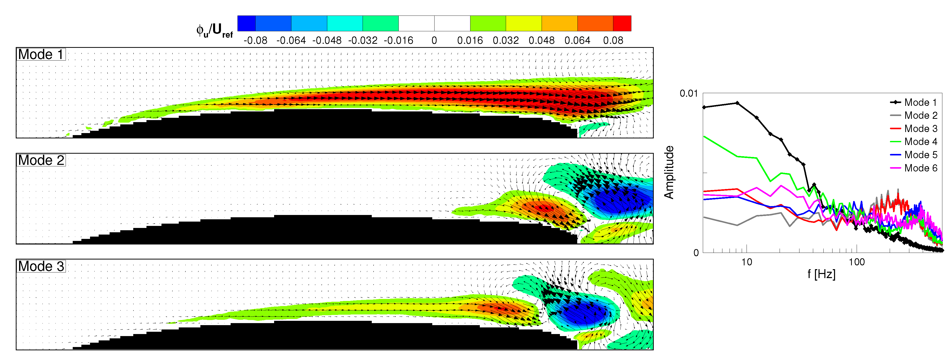
The most energetic POD modes (Figure 5, left) provide the statistical representation of the large scale structures responsible for the phase-averaged flow field just observed, as also discussed in Bourgeois et al. [
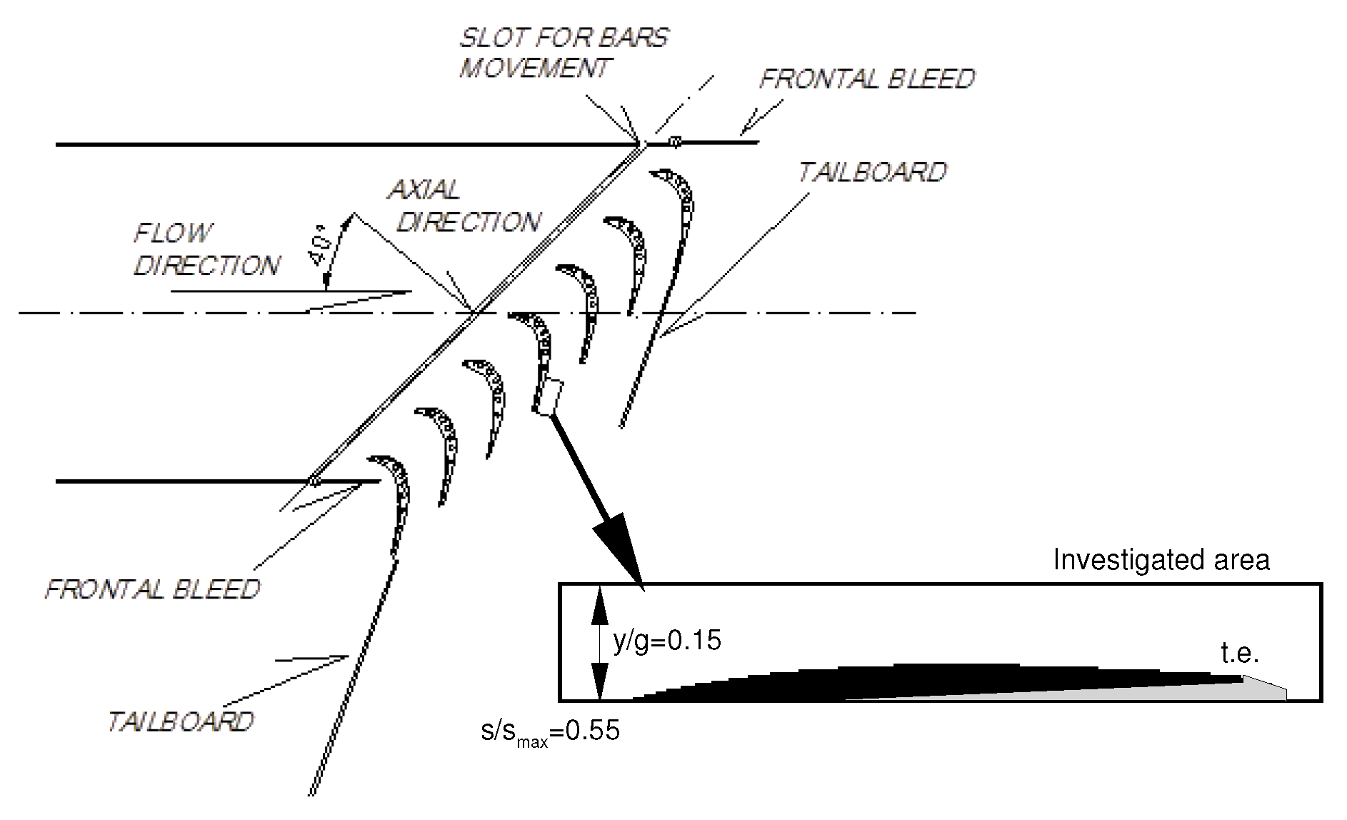
16] for the interpretation of the POD modes computed in the periodic pattern characterizing the wake of a square cylinder. It is worth noting that the POD modes and all the following pictures concern the boundary layer restricted plane (as depicted in Figure 1), which is indicated by the black box in Figure 4 for a fast comparison. The vectorial representation shows the POD mode of the two velocity components. The Fourier analysis of the temporal eigenvector (right of Figure 5) allows identifying passing wake related modes through the occurrence of distinct peaks at the wake passing frequency and higher harmonics.
For the nominal reduced frequency, the first two POD modes depict the velocity perturbation induced by the large scale structures of the wake on the boundary layer. The first POD mode appears similar to the phase averaged representation at the time t / T = 0.5 , while the second POD mode to that at t / T = 0.25 . The Fourier spectra of their temporal coefficients are almost identical, and clearly show peaks at the wake passing frequency and higher harmonics (the temporal coefficients are two similar periodic waves shifted of 90 º ). The combination of the first two POD modes and the corresponding temporal coefficients provides the reconstructed flow field associated with the periodic motion (i.e., the phase-averaged flow field). Indeed, at the instant when the temporal coefficient of one of the two POD modes is zero, the other mode directly describes the phase-averaged periodic flow map. However, the capability of POD goes beyond the identification of passing wake related effects. Indeed, the third mode in Figure 5 evidently provides the statistical representation of oscillations not observed in the phase averaged flow field. This mode, according to the Fourier analysis, is poorly associated with the wake passing events, since it shows an amplitude peak at frequencies lower than the wake passing one as well as a smaller peak at the wake passing frequency. Consequently, mode 3 only marginally contributes to the phase-averaged flow field, and it mainly describes the low frequency velocity fluctuations due to elongated structures (i.e., streaky structures) contributing to the boundary layer transition process, similarly to the results shown in a recent authors’ publication [17]. The POD analysis of the steady case shown in Figure 6 makes evident the “boundary layer nature” of this mode. Indeed, the first POD mode of this last case is almost identical to the third mode of the nominal unsteady case. The shape of this mode is the trace of streaky structures inside the suction side boundary layer generating as a consequence of the high free-stream turbulence level, as also observed in Lengani and Simoni [17]. The following modes represent alternating vortical structures that are characterized by fluctuating energy in a frequency range around 200 Hz. These modes provide the statistical representation of the vortical structures shed behind the separation bubble maximum displacement position as a consequence of a Kelvin–Helmholtz instability process [28,29,30]. In the steady case, the most energetic oscillations are due to low frequency activity and the vortex shedding phenomenon, and POD clearly identifies and isolates also these mechanisms. Particularly, the Fourier analysis of mode 1 shows an amplitude peak in the low frequency range (below 100 Hz) that corresponds to that of mode 3 in the nominal f + case (note that the ordinates of the Fourier spectra of Figure 5 and Figure 6 are different). No oscillations can be observed far from the wall since only the homogeneous free stream turbulence travels across the potential flow region.
For completeness, the POD modes and the Fourier analysis of the eigenvectors are also reported for the halved reduced frequency condition in Figure 7. The first mode is similar to the first mode of the nominal reduced frequency case, while the second mode resembles the low frequency activity boundary layer mode. Due to the larger time available to the by-pass-like transition process to develop in between two adjacent wakes, for the halved reduced frequency, the boundary layer mode appears more linked to the wake passing frequency. Now, the third mode becomes representative of the wake jet structure, similarly to mode 2 for the nominal reduced frequency. Indeed, again due to larger distance between successive wakes, a steady-like state is able to develop, thus increasing the weight played by the boundary layer most energetic POD mode (which is now the second one). Therefore, the Fourier analysis shows that all of the first six modes are related to the wake passing frequency. Even mode 2 that clearly resembles the first mode of the steady state is then triggered by the wake passing event. In this case, higher order POD modes (shown in the next section) will be also able to trace the intermittent vortex shedding process developing between adjacent wakes. Results shown for the halved condition support the ability of POD in clearly recognizing and splitting, with their relative weight, the different phenomena that simultaneously act generating the complex unsteady flow field previously observed in Figure 3.

3.2. Turbulence Kinetic Energy Production Analysis

As discussed in the previous sections, the POD can be used to represent and split, on a statistical basis, the structures that characterize the unsteady flow field according to their energy rank. However, as discussed in the data analysis section, the POD can be also used for a further analysis step. Each POD mode can be related to a quota of the TKE production rate, and equivalently to the loss generation rate.
The following three figures (Figure 8, Figure 9, Figure 10) represent for the three cases (steady, nominal and halved f + , respectively) the production rate of TKE ( P T K E ) per POD mode. This quantity has been normalized by the cube of the reference velocity and a unitary length. The integral value of the contribution of each mode on the whole measurement domain has been also computed for each mode, and it is indicated in the figures in order to provide the weight of the different phenomena in producing losses.
The production of TKE for the steady condition (Figure 8) is mainly related to the Reynolds shear stresses caused by the vortical structures originating from the boundary layer separation, except for the first POD mode. The first mode, as previously observed, is related to low frequency fluctuations of the whole boundary layer region due to streaky structures. However, the integral TKE production rate of this mode is lower than that of the modes related to the vortical structures, since, in this case, the Kelvin-Helmholtz (KH) vortices represent the dominant dynamic producing losses. TKE is mainly produced within the braid region between adjacent vortices, due to the high shear effects (long vectors pointing in the second and fourth quadrant) inducing negative shear stress. Modes 2 and 3 show vortices of the dimension of the boundary layer thickness, while modes 4–6 highlight structures of smaller dimension. Interestingly, local back-scatter can be observed (blue area in the plots) in the finer structures, where the vectors point in the first and third quadrants. As expected, for the steady case, all the sources of losses are confined in the boundary layer region, with the greatest amount of TKE production due to the boundary layer separation related events.
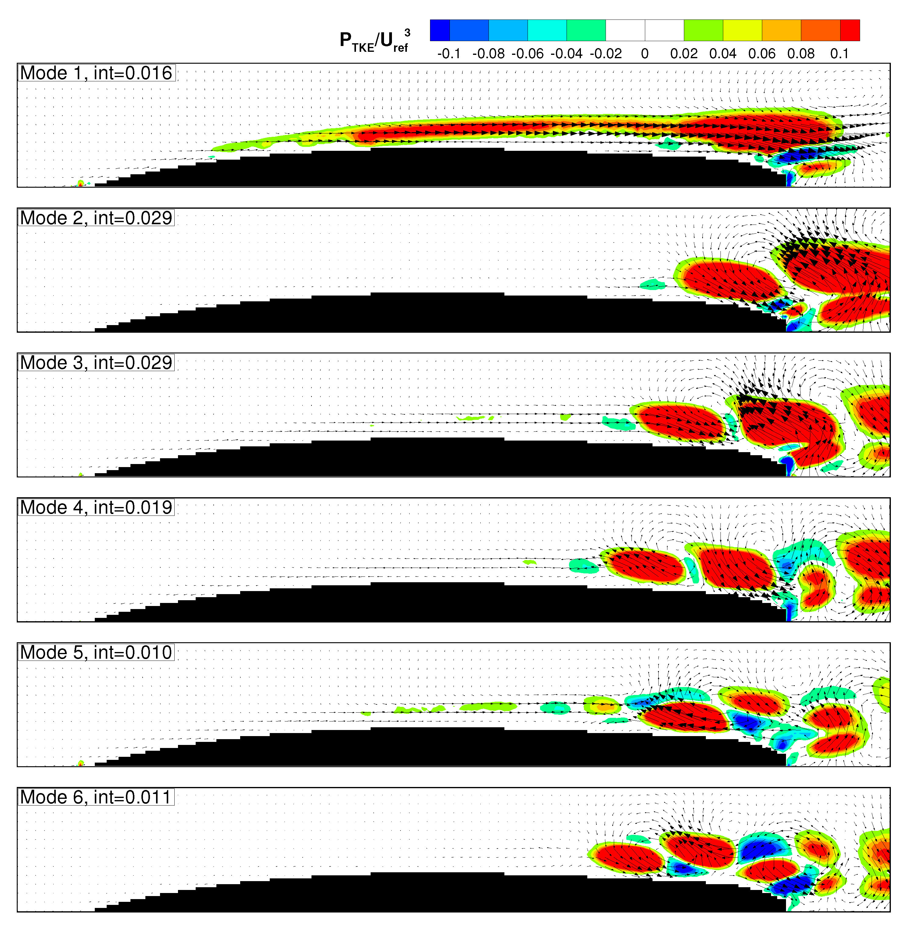
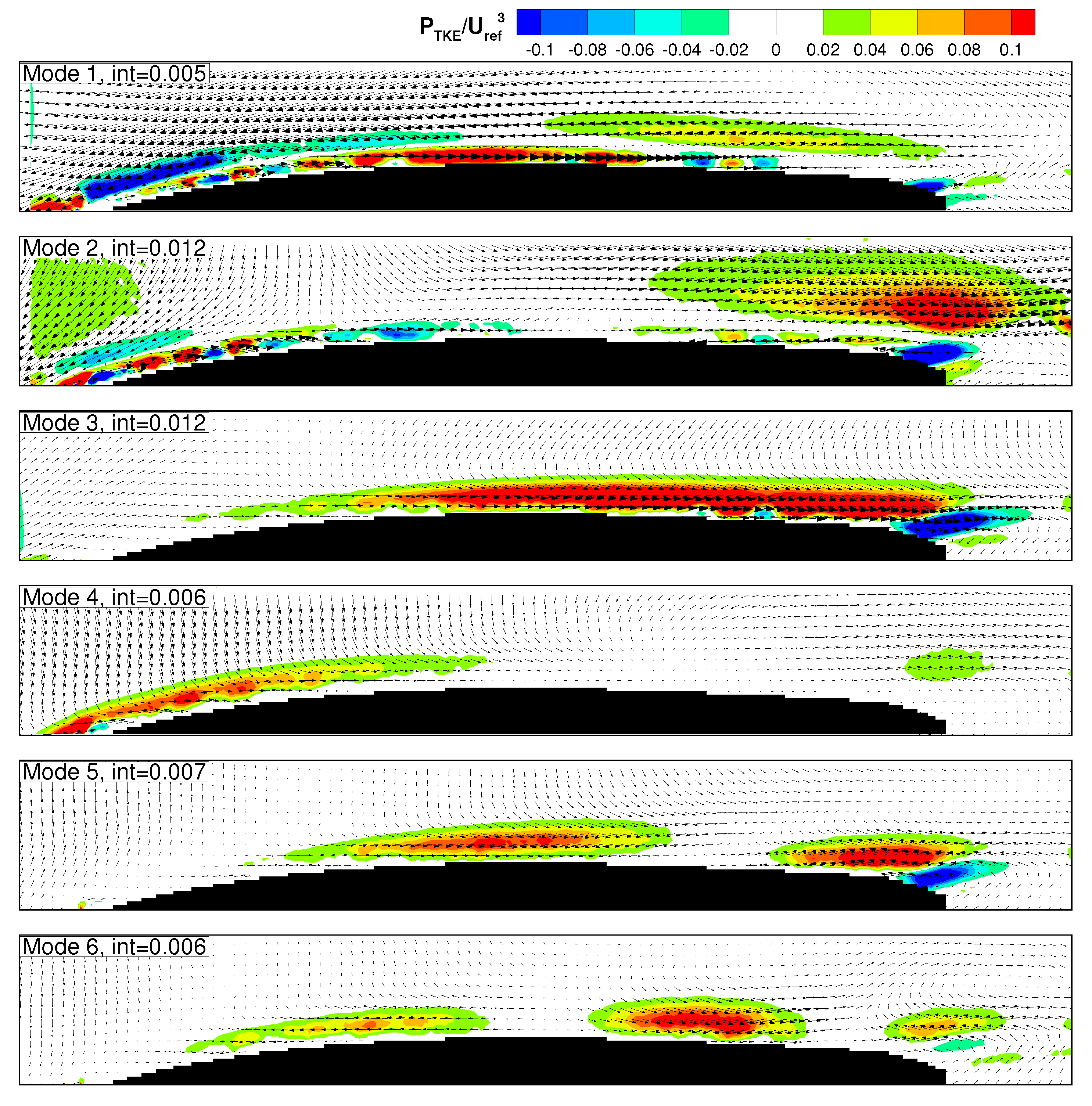
The unsteady case with nominal f + (Figure 9) presents a completely different scenario. The first two modes, related to the large scale structures of the wake, have a lower production rate of TKE with respect to the steady case (being representative of different dynamics). For these modes, the largest production is found within the boundary layer in the region where the roll up vortices caused by the interaction of the wake leading boundary and the boundary layer were previously observed. Significant losses can also be observed in mode 2 at the edge of the boundary layer extending also into the potential flow region, in the surroundings of the end of the profile surface and at the entrance of the measuring domain. This source of losses is due to the deformation of the wake patch during migration (as also described in Michelassi et al. [5]), which consequently further contributes to the overall losses in the unsteady operation of the LPT cascade. However, in the boundary layer region, the contribution due to the wake related modes together (1 and 2) to the TKE generation rate is lower than the contribution due to the boundary layer related events (modes above 2). Particularly, the third mode gives the largest production rate within the measurement domain. The TKE production into the boundary layer due to modes 3–6 appears significant also in the fore part of the measuring plane as a consequence of the by-pass like transition process forced by the incoming wakes that induces fluctuations also in this part of the suction side. Moreover, in this case, no vortex-like structures are responsible for losses, according to the absence of separation. In addition, regions of negative values of P T K E appear in the plot. Here, the TKE is reconverted to mean flow energy, i.e., back-scatter occurs.
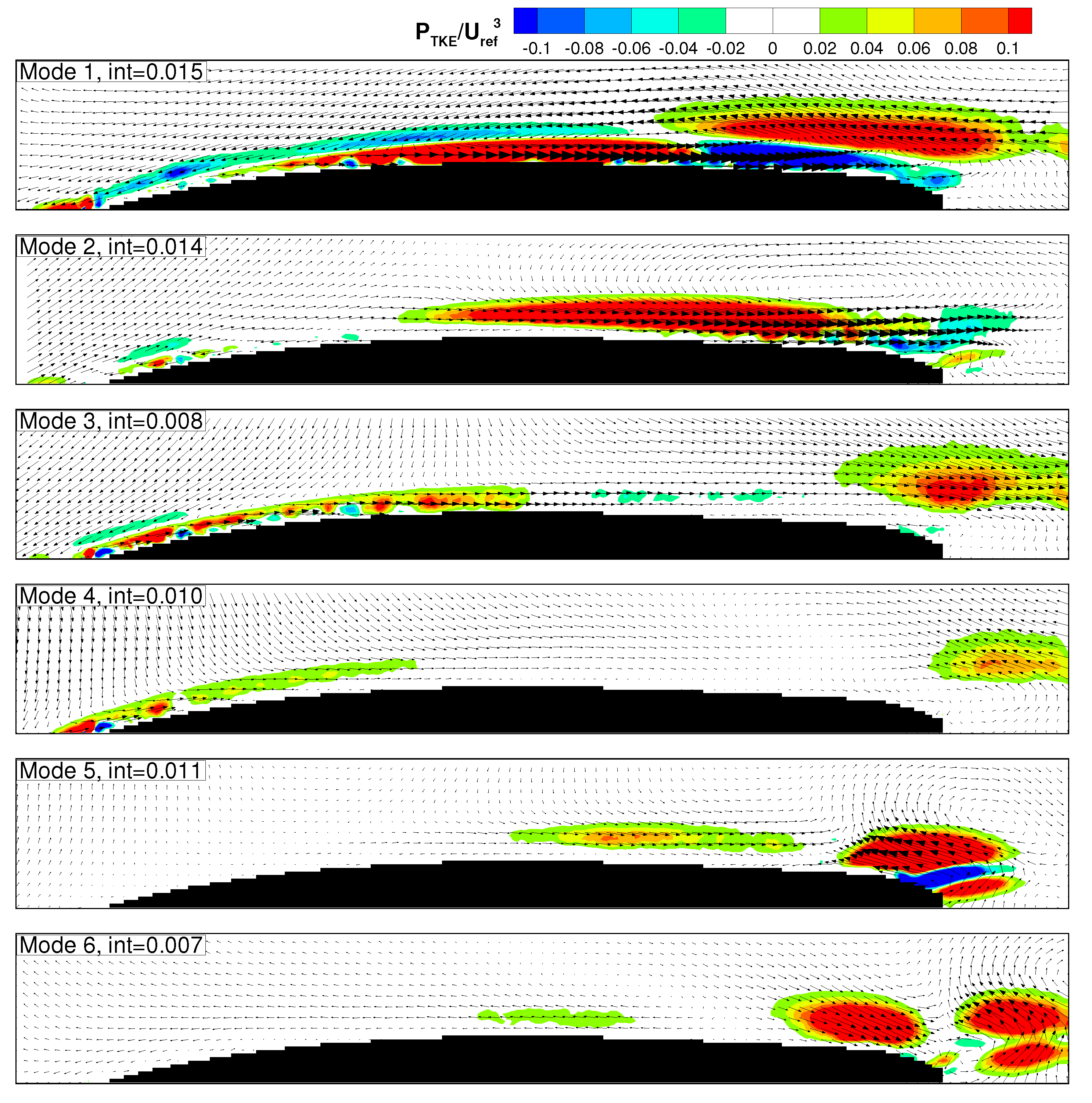
The halved f + case shows features of both the previously described cases. The TKE production rate distribution of modes 1, 3 and 4 is similar to that of modes 1, 2 and 4 of the nominal f + case. The TKE generation rate (integrated value) related to the large scale structures of the incoming wake for the halved f + (modes 1 and 3) is higher than for the nominal case. This is because the roll up vortex caused by the interaction of the wake and the boundary layer is larger for this condition, according to the thicker boundary layer developing between wakes [11]. Mode 2 (the boundary layer mode) shows losses intermediate between their counterpart for the steady (mode 1) and the nominal unsteady case (mode 3). Modes 5 and 6 are instead related to the dynamics of the unsteady separation since they clearly represent vortical structures shed in the rear part of the blade suction side. The TKE generation rate due to these modes is reduced for this unsteady case with respect to the steady one, according to the intermittent nature of the flow separation.
In order to provide a quantitative picture of the TKE produced in the three different tested conditions, the contributions per mode to the generation of TKE (Equation (8)) have been integrated in the 2D measurement domain. The results of the integration are reported in Figure 11, where the cumulative contributions have been normalized by the total production of TKE evaluated in the steady case. The cumulative contribution of the total turbulence production rate per POD mode of the steady case (black line) shows that the first 10 POD modes capture about 70% of the total, while the integration up to the 100th mode provides more than 90% of the total. This simply reflects the fact that the largest production is caused by the large scale vortical structures related to the boundary layer separation.
The total production for the unsteady case is lower for the nominal f + case, while the halved f + case stay in between the other two cases. For the unsteady cases, the first ten modes produce a lower percentage of the total when compared with the steady case. Hence, the TKE generation is related to higher order POD modes that typically are related to smaller scale stochastic structures. The halved f + case presents a steep increase of the TKE production at modes 5–9, which, as previously shown, are related to the intermittent flow separation. Hence, in the rear part of the blade suction side, the suppression of the laminar separation for the unsteady case clearly reduces the losses generated in the boundary layer.

4. Conclusions

In the present work, POD has been applied to TR-PIV data in order to characterize the different phenomena responsible for TKE production affecting the unsteady behavior of an LPT blade. The ability of POD in identifying the most important dynamics responsible for flow oscillations in the steady and in the unsteady cases has been highlighted by means of comparisons with time resolved and phase-averaged vector maps. In the steady case, POD modes evidently represent the low frequency elongated oscillations as well as the vortical structures shed as a consequence of the boundary layer laminar separation occurring in this condition. For the unsteady cases, the most energetic POD modes describe (statistically) the negative jet effects. The combination of the first two modes reproduces the phase-averaged flow field. The analysis of two different reduced frequencies strengthens the ability of POD. Indeed, in the case of the halved reduced frequency, POD modes have been shown to be able to capture superposed phenomena typical of both the steady and the unsteady operations, such as the wake migration and boundary layer separation induced effects. A TKE production split procedure, based on the biorthogonality condition of the POD modes and related temporal coefficients, allowed the quantification of the weight of each dynamic to the loss production rate. In the steady case, losses are mainly due to the vortex shedding phenomenon, while in the unsteady case the rollup vortex generated during the wake–boundary layer interaction has been found to be the dynamic with higher losses. This latter appears sensibly influenced by the reduced frequency, with higher contribution for the halved reduced frequency condition due to a thicker boundary layer developing between wakes. The clear identification of the dynamics, the estimation of their weight and the localization of the flow region where they act in producing losses may contribute in the future to the development of optimization strategies for high lift profile cascades operating under realistic unsteady flow conditions.

Acknowledgments

The authors would like to thank GE Avioaero SRL (Torino, Italy) for the financial support.

Author Contributions

D. Lengani and D. Simoni analyzed the data and wrote the paper; D. Simoni performed the experiments; D. Lengani performed the post-processing of the data; M. Ubaldi and P. Zunino supervised the work; F. Bertini provided the experiment guidelines.

Conflicts of Interest

The authors declare no conflict of interest.

Nomenclature

cblade chord
ffrequency
f b a r bar passing frequency
f + wake reduced frequency = f b a r c / u 2 , i s
gpitch
hblade height
LPTlow pressure turbine
P T K E turbulence kinetic energy production rate
R e Reynolds number = c u 2 , i s / ν
scurvilinear coordinate
s M A X trailing edge curvilinear coordinate
ttime
Twake passing period
TKEturbulence kinetic energy
ustreamwise velocity component
u 2 , i s isentropic velocity at cascade outlet
u 2 , x axial velocity at cascade outlet
U r e f reference streamwise velocity
U b a r bar rotation velocity
vnormal to the wall velocity component
xcascade axial coordinate
ynormal to the wall direction
δ boundary layer thickness
λ ( k ) POD eigenvalue of mode k
χ ( k ) POD eigenvectors of mode k
φ flow coefficient = u 2 , x / U b a r
ϕ u POD mode of the streamwise velocity component
ϕ v POD mode of the wall normal velocity component
< > deterministic periodic component
Subscripts and Superscripts
R M S root mean square
-time averaged quantities
phase-locked quantities
stochastic fluctuating component

References

  1. Mayle, R.E. The Role of Laminar-Turbulent Transition in Gas Turbine Engines. J. Turbomach. 1991, 113, 509–537. [Google Scholar] [CrossRef]
  2. Gompertz, K.A.; Bons, J.P. Combined Unsteady Wakes and Active Flow Control on a Low-Pressure Turbine Airfoil. J. Propul. Power 2011, 27, 990–1000. [Google Scholar] [CrossRef]
  3. Hodson, H.P.; Howell, R.J. The Role of Transition in High-Lift Low-Pressure Turbines for Aeroengines. Prog. Aerosp. Sci. 2005, 41, 419–454. [Google Scholar] [CrossRef]
  4. Stieger, R.D.; Hodson, H.P. The Unsteady Development of a Turbulent Wake through a Downstream Low-Pressure Turbine Blade Passage. J. Turbomach. 2005, 127, 388–394. [Google Scholar] [CrossRef]
  5. Michelassi, V.; Chen, L.W.; Pichler, R.; Sandberg, R.D. Compressible Direct Numerical Simulation of Low-Pressure Turbines-Part II: Effect of Inflow Disturbances. J. Turbomach. 2015, 137, 071005. 1–12. [Google Scholar] [CrossRef]
  6. Nagabhushana Rao, V.; Tucker, P.; Jefferson-Loveday, R.; Coull, J. Large eddy simulations in low-pressure turbines: Effect of wakes at elevated free-stream turbulence. Int. J. Heat Fluid Flow 2013, 43, 85–95. [Google Scholar] [CrossRef]
  7. Wu, X.; Jacobs, R.G.; Hunt, J.C.; Durbin, P.A. Simulation of boundary layer transition induced by periodically passing wakes. J. Fluid Mech. 1999, 398, 109–153. [Google Scholar] [CrossRef]
  8. Lengani, D.; Simoni, D.; Ubaldi, M.; Zunino, P.; Bertini, F. Coherent Structures Formation During Wake-Boundary Layer Interaction on a LP Turbine Blade. Flow Turbul. Combust. 2017, 98, 57–81. [Google Scholar]
  9. Coull, J.D.; Hodson, H.P. Unsteady boundary-layer transition in low-pressure turbines. J. Fluid Mech. 2011, 681, 370–410. [Google Scholar] [CrossRef]
  10. Pacciani, R.; Marconcini, M.; Arnone, A.; Bertini, F. URANS analysis of wake-induced effects in high-lift, low Reynolds number cascade flows. In Proceedings of the ASME Turbo Expo 2012: Turbine Technical Conference and Exposition, Copenhagen, Denmark, 11–15 June 2012. [Google Scholar]
  11. Satta, F.; Simoni, D.; Ubaldi, M.; Zunino, P.; Bertini, F. Loading Distribution Effects on Separated Flow Transition of Ultra-High-Lift Turbine Blades. J. Propul. Power 2014, 30, 845–856. [Google Scholar] [CrossRef]
  12. Shi, L.L.; Liu, Y.Z.; Wan, J.J. Influence of wall proximity on characteristics of wake behind a square cylinder: PIV measurements and POD analysis. Exp. Therm. Fluid Sci. 2010, 34, 28–36. [Google Scholar] [CrossRef]
  13. Ben Chiekh, M.; Michard, M.; Guellouz, M.S.; Béra, J.C. POD analysis of momentumless trailing edge wake using synthetic jet actuation. Exp. Therm. Fluid Sci. 2013, 46, 89–102. [Google Scholar] [CrossRef]
  14. van Oudheusden, B.W.; Scarano, F.; van Hinsberg, N.P.; Watt, D.W. Phase-resolved characterization of vortex shedding in the near wake of a square-section cylinder at incidence. Exp. Fluids 2005, 39, 86–98. [Google Scholar] [CrossRef]
  15. Perrin, R.; Braza, M.; Cid, E.; Cazin, S.; Barthet, A.; Sevrain, A.; Mockett, C.; Thiele, F. Obtaining phase averaged turbulence properties in the near wake of a circular cylinder at high Reynolds number using POD. Exp. Fluids 2007, 43, 341–355. [Google Scholar] [CrossRef]
  16. Bourgeois, J.; Noack, B.; Martinuzzi, R. Generalized phase average with applications to sensor-based flow estimation of the wall-mounted square cylinder wake. J. Fluid Mech. 2013, 736, 316–350. [Google Scholar] [CrossRef]
  17. Lengani, D.; Simoni, D. Recognition of coherent structures in the boundary layer of a low-pressure-turbine blade for different free-stream turbulence intensity levels. Int. J. Heat Fluid Flow 2015, 54, 1–13. [Google Scholar] [CrossRef]
  18. Lengani, D.; Simoni, D.; Ubaldi, M.; Zunino, P. POD analysis of the unsteady behavior of a laminar separation bubble. Exp. Therm. Fluid Sci. 2014, 58, 70–79. [Google Scholar] [CrossRef]
  19. Kurelek, J.W.; Lambert, A.R.; Yarusevych, S. Coherent Structures in the Transition Process of a Laminar Separation Bubble. AIAA J. 2016, 54, 2295–2309. [Google Scholar] [CrossRef]
  20. Sarkar, S. Identification of flow structures on a LP turbine blade due to periodic passing wakes. J. Fluids Eng. 2008, 130. 061103. [Google Scholar] [CrossRef]
  21. Simoni, D.; Berrino, M.; Ubaldi, M.; Zunino, P.; Bertini, F. Off-Design Performance of a Highly Loaded Low Pressure Turbine Cascade Under Steady and Unsteady Incoming Flow Conditions. J. Turbomach. 2015, 137, 071009. [Google Scholar] [CrossRef]
  22. Sciacchitano, A.; Neal, D.R.; Smith, B.L.; Warner, S.O.; Vlachos, P.P.; Wieneke, B.; Scarano, F. Collaborative framework for PIV uncertainty quantification: comparative assessment of methods. Meas. Sci. Technol. 2015, 26, 074004. [Google Scholar] [CrossRef]
  23. Wieneke, B. PIV uncertainty quantification from correlation statistics. Meas. Sci. Technol. 2015, 26, 074002. [Google Scholar] [CrossRef]
  24. Sirovich, L. Turbulence and the dynamics of coherent structures. Part I-III. Quart. Appl. Math. 1987, 45, 561–590. [Google Scholar] [CrossRef]
  25. Lacarelle, A.; Faustmann, T.; Greenblatt, D.; Paschereit, C.O.; Lehmann, O.; Luchtenburg, D.M.; Noack, B.R. Spatiotemporal Characterization of a Conical Swirler Flow Field Under Strong Forcing. J. Eng. Gas Turbines Power 2009, 131, 031504. [Google Scholar] [CrossRef]
  26. Mahallati, A.; Sjolander, S.A. Aerodynamics of a low-pressure turbine airfoil at low-reynolds numbers: Part 2—blade-wake interaction. In Proceedings of the ASME Turbo Expo 2007: Power for Land, Sea, and Air, Montreal, QC, Canada, 14–17 May 2007; pp. 1025–1037. [Google Scholar]
  27. Opoka, M.M.; Hodson, H.P. Experimental investigation of unsteady transition processes on high-lift t106a turbine blades. J. Propul. Power 2008, 24, 424–432. [Google Scholar] [CrossRef]
  28. Yarusevych, S.; Kotsonis, M. Effect of Local DBD Plasma Actuation on Transition in a Laminar Separation Bubble. Flow Turbul. Combust. 2017, 98, 195–216. [Google Scholar] [CrossRef]
  29. Wen, X.; Tang, H.; Duan, F. Interaction of in-line twin synthetic jets with a separated flow. Phys. Fluids 2016, 28, 043602. [Google Scholar] [CrossRef]
  30. Yarusevych, S.; Kotsonis, M. Steady and transient response of a laminar separation bubble to controlled disturbances. J. Fluid Mech. 2017, 813, 955–990. [Google Scholar] [CrossRef]
Figure 1. Schematic of the test section and particle image velocimetry (PIV) investigated area.
Ijtpp 02 00017 g001
Figure 2. Time-mean streamwise velocity component. From top to bottom: steady inlet flow case, nominal reduced frequency, half-reduced frequency. The dividing streamline is traced by the dashed white line for the steady case.
Ijtpp 02 00017 g002
Figure 3. Time series of the instantaneous perturbation velocity, 0.5 f + case. The time interval between each snapshot is 0.06 of the wake passing period (five times larger than the time-resolved particle image velocimetry (TR-PIV) temporal resolution).
Ijtpp 02 00017 g003
Figure 4. Phase-averaged velocity vector maps with superimposed the streamwise velocity contour for the nominal f + .
Ijtpp 02 00017 g004
Figure 5. The proper orthogonal decomposition (POD) modes (left) and Fourier spectra of POD eigenvectors (right) for the nominal f + case.
Ijtpp 02 00017 g005
Figure 6. The POD modes (left) and Fourier spectra of POD eigenvectors (right) for the steady case.
Ijtpp 02 00017 g006
Figure 7. The POD modes (left) and Fourier spectra of POD eigenvectors (right) for the halved f + case.
Ijtpp 02 00017 g007
Figure 8. Turbulence kinetic energy production rate per POD mode, steady case.
Ijtpp 02 00017 g008
Figure 9. Turbulence kinetic energy production rate per POD mode, nominal f + case.
Ijtpp 02 00017 g009
Figure 10. Turbulence kinetic energy production rate per POD mode, halved f + case.
Ijtpp 02 00017 g010
Figure 11. Cumulative contribution to the TKE production rate of each POD mode. The values are obtained by integration over the 2D measurement domain.
Ijtpp 02 00017 g011

