Article

A Comparative Study of Varying Incidence Angle Effects on a Low-Reynolds-Number Compressor Cascade Based on Experiments and Low-Fidelity and High-Fidelity Numerical Simulations †

1
Institute of Propulsion Technology, German Aerospace Center (DLR), Linder Höhe, 51147 Cologne, Germany
2
Institute of Test and Simulation for Gas Turbines, German Aerospace Center (DLR), Linder Höhe, 51147 Cologne, Germany
*
Author to whom correspondence should be addressed.
This manuscript is an extended version of the ETC2025-231 meeting paper published in the Proceedings of the 16th European Turbomachinery Conference (ETC16), Hannover, Germany, 24–28 March 2025.
Int. J. Turbomach. Propuls. Power 2025, 10(4), 42; https://doi.org/10.3390/ijtpp10040042
Submission received: 17 July 2025 / Revised: 14 August 2025 / Accepted: 14 August 2025 / Published: 4 November 2025

Abstract

The trend towards higher bypass ratios and downsized cores in modern compressors leads to locally reduced Reynolds numbers, intensifying flow separation and unsteadiness, which limits the reliability of RANS models and motivates the use of LES as a feasible and attractive high-fidelity approach for these conditions. In this paper, we assess the capabilities of low- and high-fidelity numerical tools for predicting the effects of varying incidence angles for a linear compressor cascade at a Reynolds number of 150,000 and a Mach number of 0.6 based on the inflow conditions. The comparison is supported by experiments carried out at the Transonic Cascade Wind Tunnel at the DLR in Cologne, which feature an incidence angle variation of plus/minus 5 degrees. Particular emphasis is put on the numerical setup to reproduce the cascade experiment, discussing the effects of spanwise domain size, axial-velocity density ratio and inflow turbulence. The effects of the incidence angle variation are studied on the basis of instantaneous and mean flow quantities with a focus on separation, transition and loss mechanisms.

Graphical Abstract

1. Introduction

Efficiency improvements are one key aspect to meet the challenging governmental requirements for climate-neutral aviation. Design is trending towards even higher bypass ratios and, as a result of limited clearance underneath the aircraft wings, towards more powerful and smaller core engines. Besides more pronounced secondary flow effects, this also results in locally reduced Reynolds numbers ( Re 10 5 ) in axial compressor stages [1]. At these low Reynolds numbers, airfoil aerodynamics becomes critical and losses can increase due to laminar or turbulent boundary layer separation. The airfoil aerodynamics at these operating points can also be subject to long and unsteady separation bubbles on the suction and/or pressure side of the blade, transition from laminar to turbulent boundary layers and a significant vortex shedding depending on the incidence angle. In off-design conditions with increasing incidence angles, the load on the boundary layers rises, resulting in moderately higher losses. Eventually, the airfoil reaches a point where it can no longer achieve the required pressure rise, leading to flow separation on the suction side and a sharp increase in the loss coefficient. A similar trend occurs for negative incidence angles, where the risk of pressure-side separation grows. This behavior is characteristic of blades operating under subsonic conditions [1,2,3].
The state-of-the-art design methodologies for axial compressor blades, such as multi-fidelity optimization processes using Reynolds-averaged Navier–Stokes (RANS) simulations as a ‘high-fidelity’ tool [4,5], can become unreliable at off-design points. This is because RANS, despite being considered high-fidelity, is susceptible to significant modeling uncertainties under challenging operating conditions, which might lead to over-predicted profile losses and misrepresentation of parameter trends. For instance, Hergt et al. [1] demonstrated that while RANS performs well within the typical design range of high Reynolds numbers, it fails to accurately predict loss trends and the static pressure rise at lower Reynolds numbers.
Unlike RANS, scale-resolving simulations such as direct numerical simulation (DNS) and large-eddy simulation (LES) capture all or most of the turbulent scales, respectively, and thus benefit from significantly reduced modeling uncertainty. Numerous publications in recent years have demonstrated that these methodologies perform well for compressor and turbine cascades and, when properly configured, can be as reliable as experimental data [6,7,8,9,10]. Scale-resolving simulations are especially well suited to flows with a low Reynolds number, as the required computational resources remain moderate [11], and depending on the case and solver properties, LES can be performed within some hours of wall-clock time. In addition to that, LES allows for a more in-depth analysis of the flow due to the availability of the temporally and spatially resolved flow field. Building on these advantages, a modern high-order DG solver for LES and DNS has been developed within DLR’s standard turbomachinery flow solver TRACE over recent years [12,13], which has been extensively validated on and applied to compressor and turbine cascade flows [8,9,10,14,15].
With this new high-fidelity tool at hand, we aim to reassess the cascade presented in Hergt et al. [1] and analyze the effects of the varying incidence angles on a modern compressor cascade at an operating point with a low Reynolds number of Re 1 = 150,000 and a Mach number of Ma 1 = 0.6 . A preliminary version of this study was presented at the 16th European Turbomachinery Conference [16]. The paper starts with a detailed description of the cascade, the experimental setup and both RANS and LES setups. The effects of the spanwise domain size, axial velocity density ratio (AVDR) and inflow turbulence are discussed in terms of time- and space-averaged quantities obtained with LES for the zero-incidence-angle case. Subsequently, the results of different incidence angles, ranging from 5 deg to + 5 deg , are compared between the experiment, RANS and LES. More detail on the loss production mechanisms is given by the analysis of entropy generation in the compressor flow field.

2. Cascade Description

The compressor airfoil was originally developed as an outlet guide vane behind a low-pressure turbine stage of a small turbofan engine [17,18] and has then been further optimized for the application of riblets [19]. An overview of the general design parameters is given in Table 1, and the profile thickness and camber line angle distribution are given in Figure 1. The experiments were carried out at the Transonic Cascade Wind Tunnel [20,21] at the DLR in Cologne. The numerical simulations, i.e., RANS and LES, were performed with DLR’s solver for turbomachinery flows TRACE, which was developed in close cooperation with MTU Aero Engines AG.

2.1. Experimental Setup

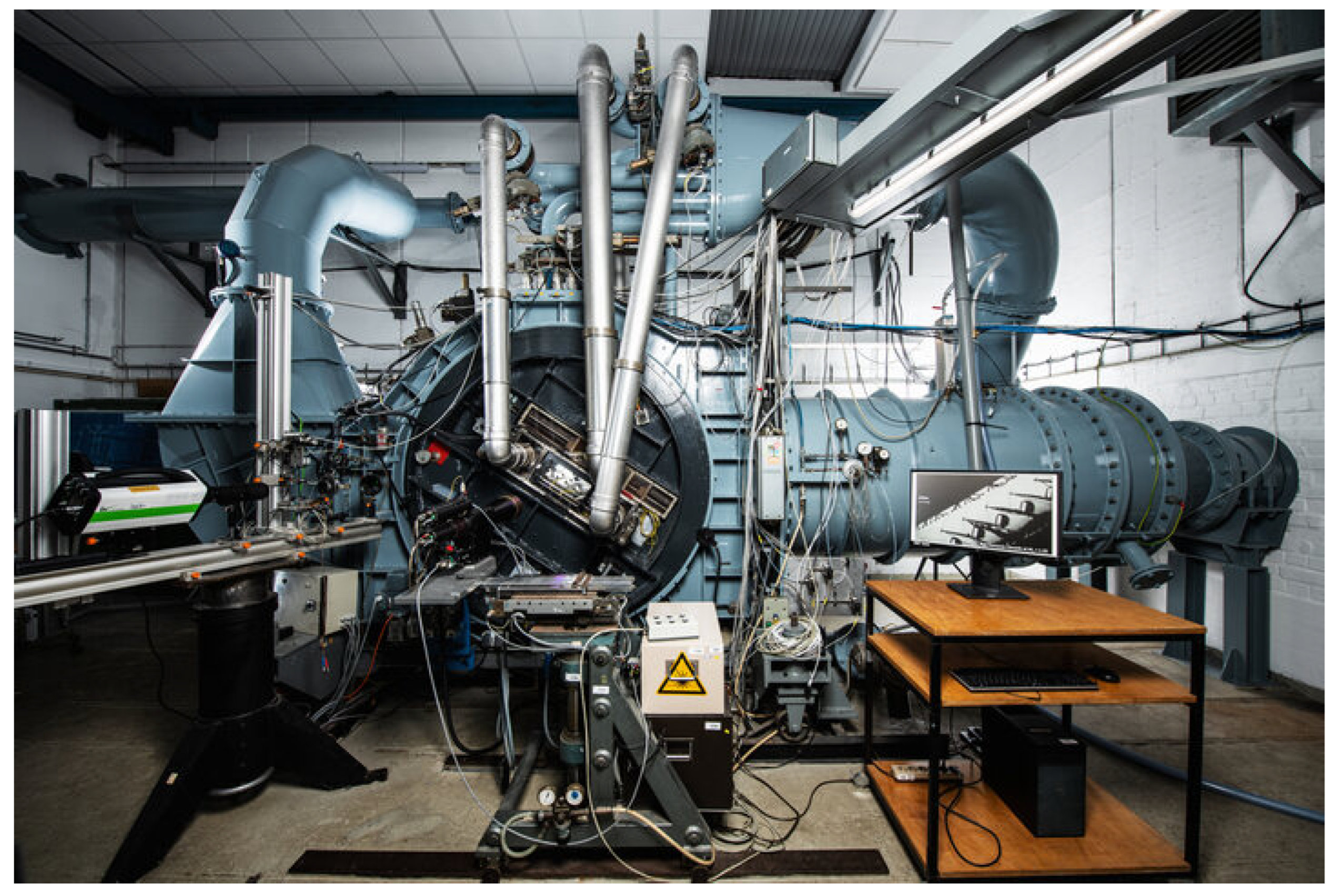
The Transonic Cascade Wind Tunnel, as shown in Figure 2, is a state-of-the-art facility for the study of compressor cascade flows and has been developed over a long period to operate in difficult flow conditions. The wind tunnel is a closed-loop facility and enables continuous testing. The test section is equipped with a variable nozzle. The variable test section height is necessary to adjust the test section for the specific cascades. Tailboards combined with throttles are used to control inlet and exit boundary conditions. In order to obtain tests at low Reynolds numbers, the total pressure in the closed-loop system of the facility is reduced.
Within the experimental campaign, the cascade setup consists of seven prismatic blades. Static pressure taps on the suction and pressure side surface at mid-span of blades 3 and 5 are used to determine the profile Mach number distribution. In addition, measurement planes are located 20 mm in front of the blade’s leading edge (MP1) and 20 mm downstream of its trailing edge (MP2). Conventional static pressure measurements are used at both planes. To derive the cascade loss, total pressure was measured in the settling chamber as well as in the wake at MP2 by means of a three-hole probe. Moreover, the AVDR in the cascade is controlled over boundary layer suction slots within the passages. Unfortunately, inflow turbulence was not measured during the present campaign, so we have to rely on previous measurement experiences at the test stand, which indicate turbulence intensity in the range of Tu = 0.3–0.5%, with no available information on the turbulence length scale.

2.2. RANS Setup

The RANS simulations are performed using a density-based Finite-Volume discretization on block-structured meshes. A Monotonic Upstream-centered Scheme for Conservation Laws (MUSCL) scheme with Van-Albada 1 limiter in combination with Roe’s approximate Riemann solver is used to discretize the convective fluxes, and central derivatives are employed for the viscous fluxes to obtain second-order accuracy in space. In order to derive the steady state solutions, the five conservation equations are solved in a coupled manner using an implicit dual time-stepping approach. The additional turbulence model equations are solved implicitly in a conservative but segregated manner [22]. In the present study, we employ Menter’s SST k- ω model in the version of 2003 [23], with the stagnation point fix of Kato and Launder [24]. The transition from laminar to turbulent flow is modeled by the two-equation γ - Re θ model [25]. This model combination represents a state-of-the-art setup in industrial turbomachinery CFD. At the inflow and outflow boundaries, two-dimensional non-reflecting boundary conditions are used [26]. Periodic boundary conditions are used in the pitchwise direction and inviscid walls in the spanwise direction. The effect of the AVDR is modeled via a source term affecting the mass, momentum, and energy equations
S = 1 h h x [ 0 , p , 0 , 0 , 0 ] T F adv x
following Giles [27] and Bolinches et al. [28], where p is the static pressure, h the height of the channel, x the axial coordinate and F adv x the advective flux vector in the axial direction. The contraction of the channel height is modeled from the blade’s leading edge (LE) towards the trailing edge (TE) and shaped with a sinusoidal distribution, i.e.,
h ( x ) = h LE h TE 2 cos x x LE x TE x LE π + 1 + h TE .
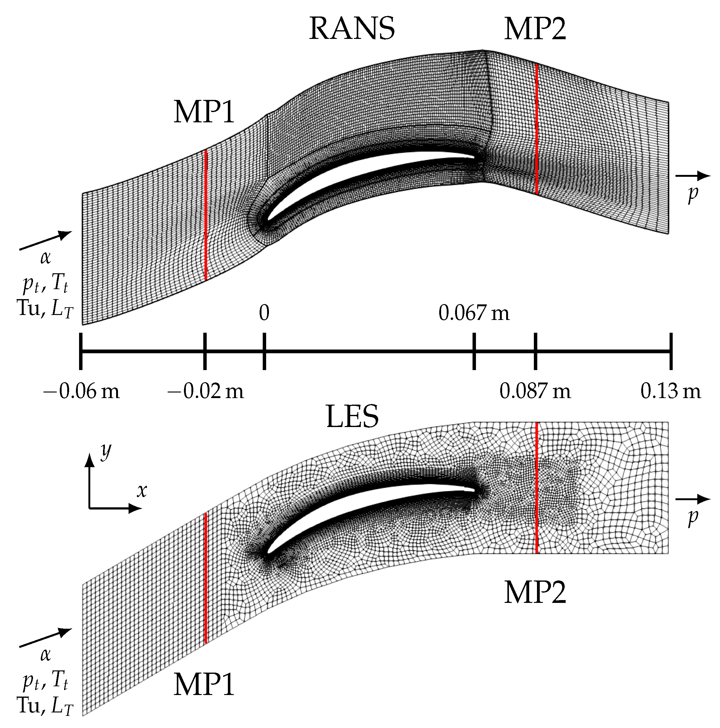
The same mesh was used for all RANS simulations. It was created with the in-house meshing tool PyMesh using an O-C-H topology [29]. The mesh consists of 70,480 hexahedral elements with one cell of height Δ ζ = 0.002 m in the spanwise direction. For the aerodynamic design point (ADP), a grid convergence index of 0.58 % and the off-design point with + 5 deg incidence angle 3.83 % is reached on the integral total pressure loss coefficient. The domain and mesh are shown in Figure 3. Probes are used to extract the mean flow values at several positions, i.e., MP1, MP2 or boundary layer cuts, ensuring consistency with the LES and experiment.

2.3. LES Setup

The LES was performed with the high-order Discontinuous Galerkin (DG) solver of TRACE, which has been developed over recent years and thoroughly validated on and successfully applied to various turbomachinery-related configurations, cf. [8,9,12,13,15]. The implicitly filtered Navier–Stokes equations are first transformed into the reference system with a high-order polynomial mapping, which ensures free-stream preservation. The solution and fluxes are approximated via one-dimensional fourth-order Legendre polynomials with Legendre–Gauss–Lobatto basis nodes, which are extended to three dimensions in a tensor-product fashion. The numerical integration is performed with Legendre–Gauss–Lobatto quadrature, collocated with the solution approximation. The viscous terms are discretized using the Bassi and Rebay 1 scheme [30]. Adjacent elements are coupled via Roe’s approximate Riemann solver for the advective part and central fluxes for the viscous part. Stabilization for under-resolved turbulent flows is achieved by using a split formulation of the Discontinuous Galerkin Spectral Element Method (DGSEM) following Gassner et al. [31]. In this present study, Kennedy and Gruber’s kinetic-energy-preserving two-point fluxes are used [32]. The resulting discretization achieves a fifth-order accuracy on unstructured hexahedral grids. The time-integration is performed by employing a strong-stability preserving third-order explicit Runge–Kutta scheme of Shu and Osher [33].
Riemann and one-dimensional non-reflecting boundary conditions are used at the inflow and outflow, respectively, cf. [26]. Inflow turbulence is generated synthetically at the inflow plane by an STG, originally proposed by Shur et al. [34], and implemented and validated in [35,36]. The STG is based on a superposition of Fourier modes, with random phases and direction vectors that produce a modified von Karman spectrum. The fluctuations of the STG are added onto the boundary state derived from the boundary conditions and are weakly imposed through the flux. Periodicity is enforced in the pitch- and spanwise directions. Similar to RANS, the source term in Equation (1) is used to model the effect of the AVDR on the mid-section. The in- and outflow boundary values, i.e., total pressure p t , in , total temperature T t , in and inflow angle α in , and the static pressure at the outflow p out , are set to the values measured in the experimental campaign of Hergt et al. [1].
The unstructured high-order mesh was created as a 2D mesh with Gmsh [37], which was then uniformly extruded in the spanwise direction. In the x-y plane, the mesh consists of 10,616 quadrilaterals. Polynomials of degree 2 have been used to approximate the curved boundary and the six layers adjacent to the wall. An overview of the 2D mesh can be found in Figure 3, which clearly demonstrates the benefit of unstructured meshes, being able to locally refine the mesh at relevant locations, i.e., boundary layer and wake region. In the spanwise direction, the resolution is kept constant for different spanwise extents, which is 24 elements and, hence, 120 degrees of freedom (DOF) per 0.1 c .
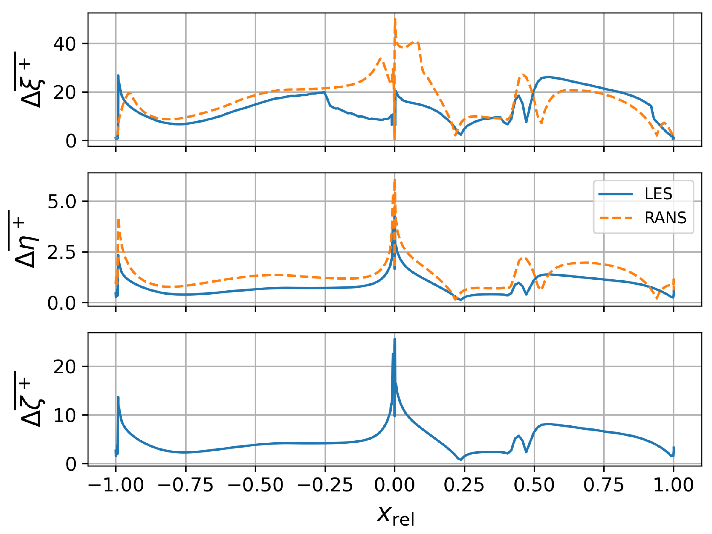
Figure 4 shows the non-dimensional cell sizes at the blade wall for the ADP. The maximum cell sizes, i.e.,
Δ ξ + ¯ 27.5 , Δ η + ¯ 2.1 , Δ ζ + ¯ 12.2 , x rel ( 0.01 , 0.99 ) ,
are well-below the limit of well-resolved LES [38]. Here, x rel is the relative coordinate along the staggered blade, which is defined by
x rel = cos arctan y x α s x 2 + y 2 c ,
where α s is the stagger angle.
Each simulation is begun from an initial RANS solution that has been interpolated onto the fine high-order grid. The LES are run for 43 t c , defined by the inflow velocity and the chord length as t c = c / | | u 1 ¯ | | . The line plots have been created with the time-resolved data of volume and boundary probes, which have been sampled with a frequency of f s = 10 6 Hz 500 / t c . The initial transient was automatically detected and removed by the MSER, cf. [39]. For entropy generation analysis, statistical moments of the full 3D flow field have been used, which have been sampled starting at 5 t c with same frequency as the probes. The computational costs per convective time unit are 4816.8 CPU/hour, which corresponds to approximately 1.25 h of wall-clock time on 3840 CPUs.

3. Analysis of the LES Setup for the Aerodynamic Design Point

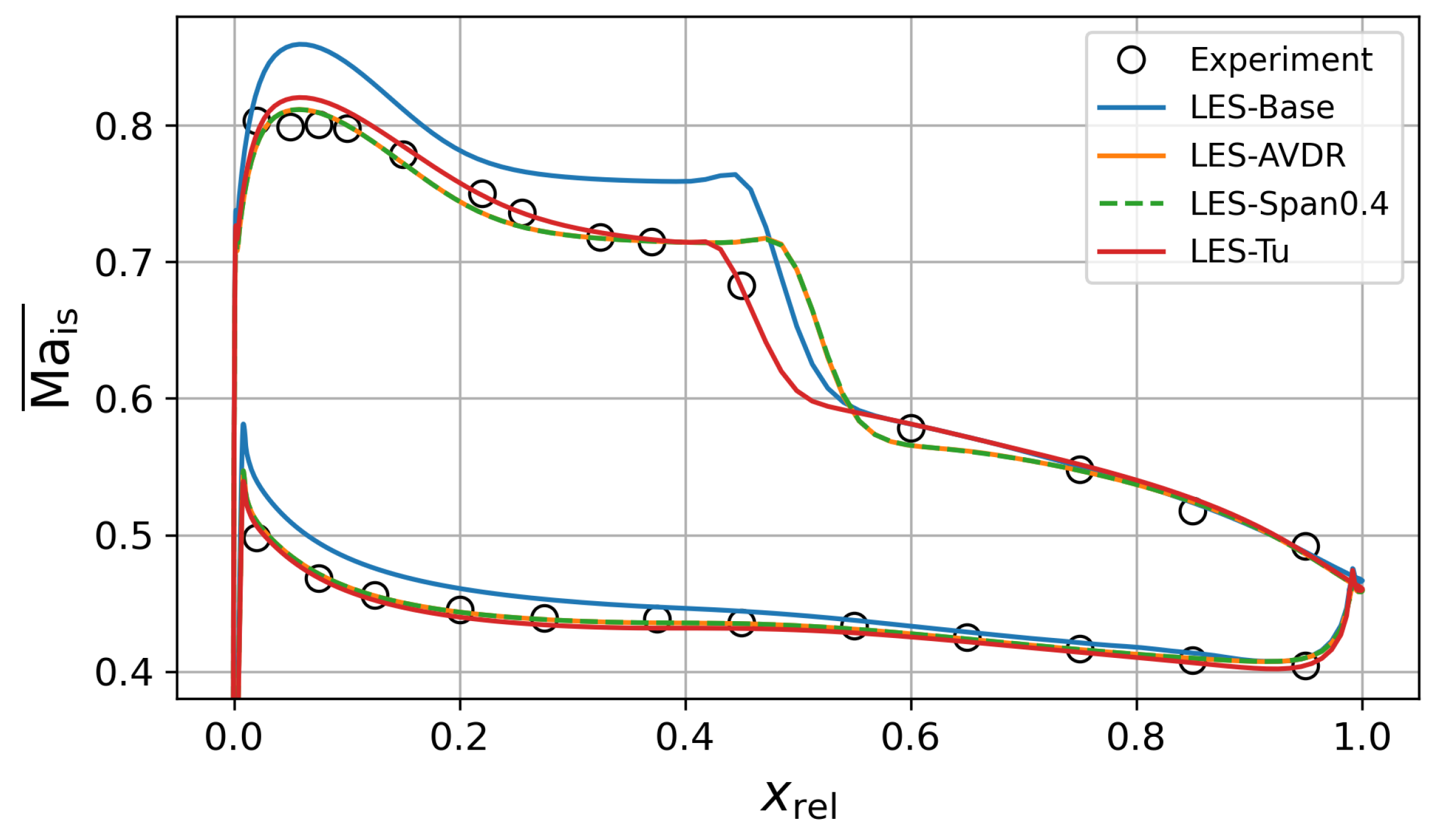
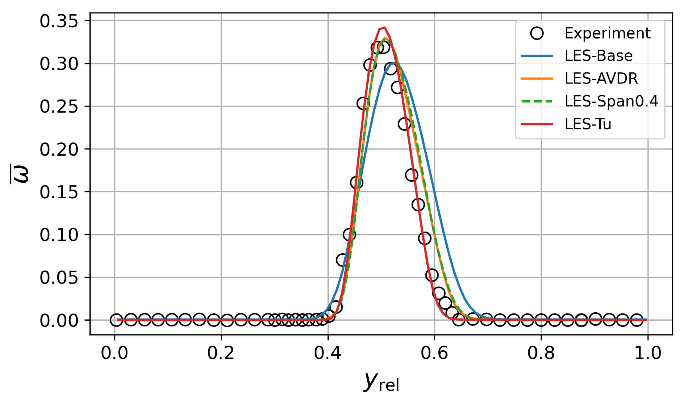
Before assessing the results of the incidence angle variation, the influence of different LES setup choices, namely the spanwise domain size, the AVDR and the inflow turbulence, are briefly discussed for the aerodynamic design point at α 1 = 43 deg . For the setups listed in Table 2, the time- and spanwise-averaged isentropic Mach number and total pressure loss coefficients with respect to MP1 are shown in Figure 5 and Figure 6, respectively. The isentropic Mach number for the LES is computed as
Ma is ¯ ( x rel ) = 2 γ 1 p t , 1 ¯ p ¯ ( x rel ) γ 1 γ 1 ,
and the total pressure loss coefficient is computed as
ω ¯ ( y rel ) = p t , 1 ¯ p t , 2 ¯ ( y rel ) p t , 1 ¯ p 1 ¯ .
Here, ¯ represents the time average and the spatial average. The wake coordinate is given by
y rel = y y LE mod b .
Since the root location of the wake measurements could not be identified with certainty, the experiments are shifted to match the peak location of the LES-Tu in the ADP.
In addition to the LES results, the experimental results of Hergt et al. [1] are shown. Starting with the LES-Base without inflow turbulence and with an AVDR equal to 1, a significant difference in the Mach number distribution compared to the experiment can be observed. Clearly, the blade loading does not match, which is also visible in the increased Mach and Reynolds numbers at MP1, cf. Table 2. With the usage of the AVDR source term (LES-AVDR), although the effective flow area was only reduced by 3.8%, the loading does improve and, overall, the LES and the experiments converge. However, the length of the separation bubble on the suction side is significantly over-predicted. Doubling the spanwise domain size to 0.4 c (LES-Span0.4) does not change the mean flow field and the isentropic Mach number and loss are identical. This can also be confirmed by the two-point correlation of the velocity components along the spanwise coordinate z, which exhibits a pronounced plateau at and above a span size of 0.2 c . Hence, a span of 0.2 c is assumed to be sufficient and will be used for the following LES.
The next parameter of uncertainty of the LES setup is the inflow turbulence, which has not been measured during the experimental campaign but is known from previous studies in the wind tunnel without turbulence grids to be between 0.3 % and 0.5 % . We chose an inflow turbulence level at the CFD inlet of 0.4 % , with a turbulence length scale of L T = 0.001 m, which fits 14 times into the spanwise domain. The distribution of the turbulence intensity along two inflow probe lines is shown in Figure 7. Here, one probe line, aligned with the inflow angle, points toward the leading edge of the blade, while the other is shifted by half a pitch. Both profiles of turbulence intensity are consistent until x / c = 0.2 , where the potential field of the blade becomes significant. At MP1, the averaged turbulence intensity is Tu 1 = 0.33 % . The effect of free-stream turbulence can be studied by vortex visualization of the instantaneous flow field close to the suction side of the profile in Figure 8. Without inflow turbulence, one can observe the typical incoming laminar boundary layer, largely consisting of 2D Kelvin–Helmholtz roll-ups (A), which transition into 3D turbulence exhibiting hairpin vortices. With inflow turbulence, even at the low level of Tu = 0.33 % , the pronounced 2D roll-ups are not present anymore (B) and the transition and reattachment are shifted upstream. This can, of course, also be observed in the Mach number distribution shown in Figure 5. The inflow turbulence significantly shortens the laminar separation bubble of the mean flow field by about 29 % . This leads to a very good agreement with the experiment, matching the sensor data in nearly all locations, except for the most upstream ones very close to the leading edge. Due to the reduced size of separation, the wake loss profile also narrows towards the wake width of the experiment, cf. Figure 6. The peak loss is slightly over-predicted but shows an overall remarkable agreement for such a sensitive quantity. It is worth noting that the inflow and outflow boundary conditions have been used directly from the experiment and were not tuned to match the operating point. Also, the inflow turbulence is well within the given experimental range. With this setup (LES-Tu) and procedure, we will discuss the variation of the inflow angle in the following section.

4. Incidence Angle Variation

In this section, the results from the experiments of Hergt et al. [1], RANS simulations and LES are compared for off-design conditions. Four additional incidence angles, i.e., 5 deg ( α 1 = 38 deg ), 3 deg ( α 1 = 40 deg ), + 3 deg ( α 1 = 46 deg ) and + 5 deg ( α 1 = 48 deg ), are considered and compared to the ADP. The inflow Mach number and Reynolds number are kept approximately constant over the angle variation. The in- and outflow boundary conditions for the simulations are taken from the experiment and are not adapted. The turbulent boundary conditions of RANS are tuned to match those of the LES. The simulation setups are shown in Table 3. Note that the experimental boundary conditions, i.e., total pressure, total temperature and flow angles at the inflow, as well as static pressure at the outflow, are directly imposed to reproduce the setup as accurately as possible. Consequently, the Mach and Reynolds numbers at MP1 result from the predicted flow characteristics within the cascade. Hence, if the loss prediction differs significantly from the experiment, the inflow Mach and Reynolds numbers also change. The instantaneous flow field for the five considered operating points is illustrated in Video S1 (Supplementary Materials).

4.1. Instantaneous Flow Field

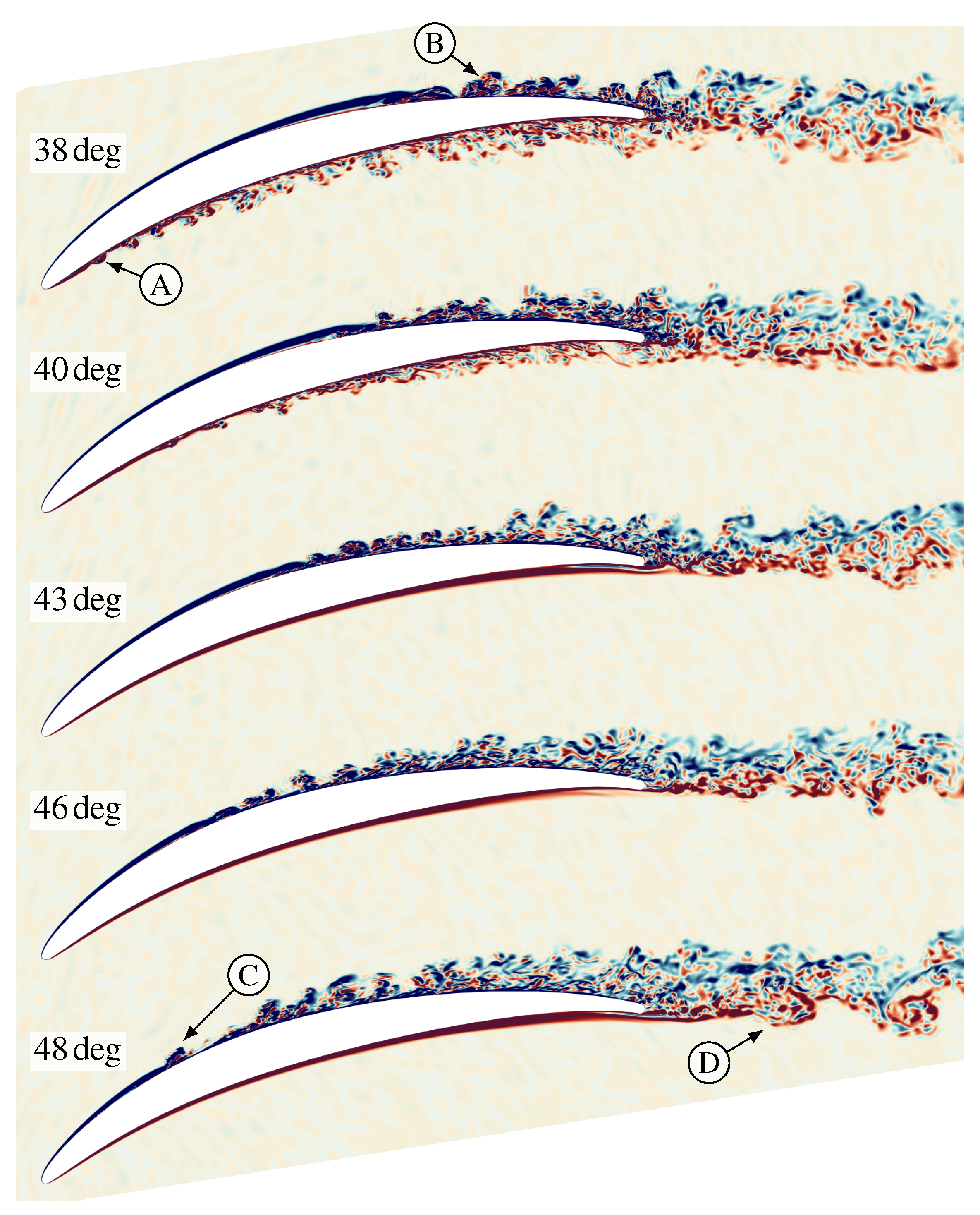
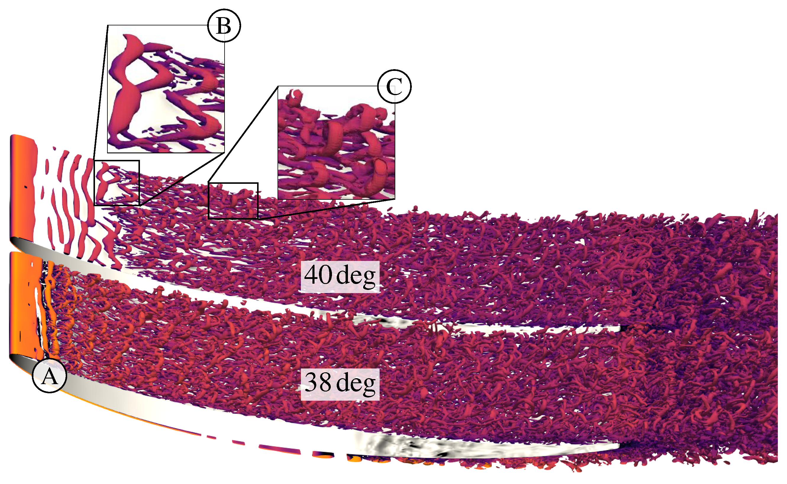
First, the instantaneous flow field of the different LES in Figure 9 is analyzed. The ADP ( α 1 = 43 deg ) is in the center of the figure, negative incidence is shown above and positive incidence is shown below. At negative incidence, the laminar pressure-side boundary layer intermittently separates for α 1 = 40 deg and transitions at x rel 0.14 . The largest negative incidence at α 1 = 38 deg exhibits a separation fixed closely to the LE (Figure 9-A), resulting in a turbulent boundary layer over nearly the complete pressure side. This is also visualized in detail in Figure 10. In the high-incidence case, typical 2D Kelvin–Helmholtz vortices are observed (Figure 10-A), which rapidly transition into a turbulent boundary layer characterized by large hairpin vortices. However, at a moderate incidence angle of 40 deg , the transition process is delayed. Spanwise-correlated roll-ups develop near the leading edge and persist over a longer extent. These roll-ups eventually lead to the formation of lambda vortices (Figure 10-B) arising from instabilities within the separated shear layer. As the flow evolves, the shear layer becomes unstable, leading to the development of these vortex structures. The lambda vortices are precursors to further breakdown processes, which ultimately result in the formation of hairpin vortices (Figure 10-C) as the flow transitions to a fully turbulent boundary layer.
Looking at the suction-side boundary layer in Figure 9, the separation is delayed due to the reduced pressure gradient. Yet, when the boundary layer separates, even larger roll-ups occur (Figure 9-B), resulting in a thickening of the turbulent wake. With a positive incidence angle, the laminar boundary layer on the suction side separates earlier (Figure 9-C), while the pressure-side boundary layer remains laminar over the whole blade. However, the shape of the blade causes large-scale oscillations leading to large 2D structures in the wake (Figure 9-D).

4.2. Blade Loading

In Figure 11, the averaged isentropic Mach number is shown for all considered inflow angles of the experiment, LES and RANS simulations. The different incidence angles are shifted on the x-axis by their index j, as noted in the text box, see Table 3. Overall, the agreement of both RANS and LES with the experiments is respectable. At the ADP, RANS predicts a very similar profile to the LES. Slight differences can be observed in the area of the suction side separation, where the reattachment position is delayed in the RANS. Moving towards positive incidence angles, this trend worsens. While the separation position is also advanced in RANS, the difference in the size of the separation compared to LES is increased and to a higher pressure plateau. Looking at the negative incidence angles, the agreement with the experiment in terms of reattachment on the suction side is weakened. While the LES still fairly closely matches the length of the bubble for α 1 = 40 deg , it is significantly over-predicted for α 1 = 38 deg . At this point, RANS seems to be closer to the experiment. Without further measurement data, the reason for the discrepancies is not clear. Inflow turbulence or inhomogeneous inflow boundary conditions could be an issue in the experiment. Yet, the pressure side separation is predicted well by the LES. Due to the pronounced unsteadiness in this region, RANS faces significant issues in reproducing the pressure distribution of the separation region, exhibiting artificial oscillations.

4.3. Skin Friction

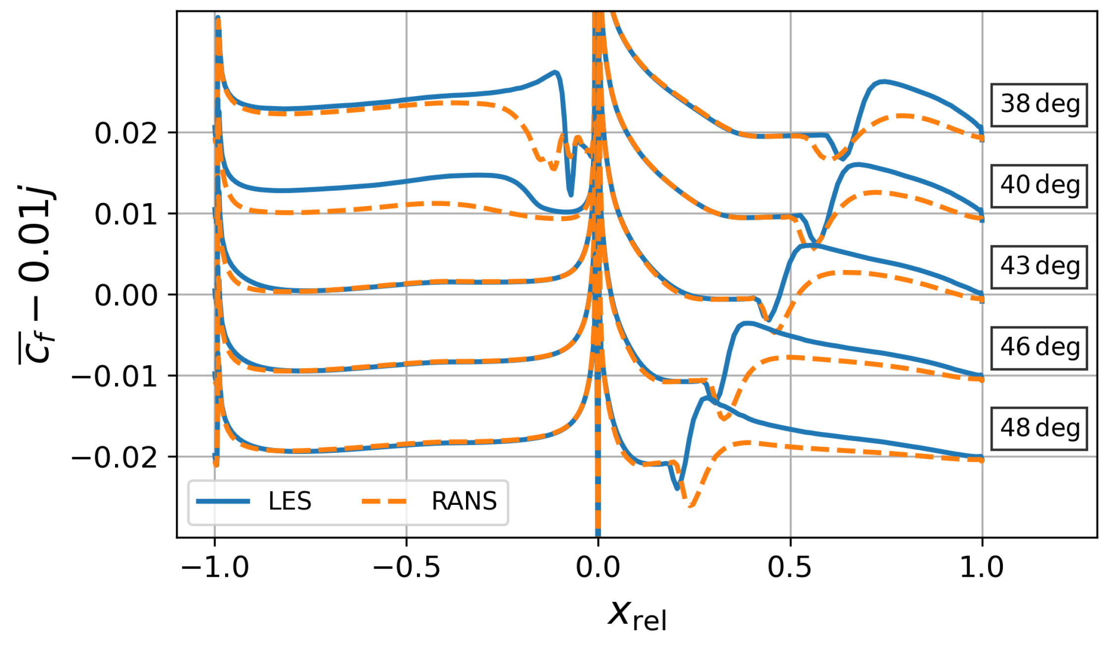
The skin friction coefficient on the blade, shown in Figure 12, underlines the observations made in the previous sections. It is defined as
c f ¯ = sign τ w , x ¯ · τ w , x ¯ 2 + τ w , y ¯ 2 + τ w , z ¯ 2 0.5 ρ in u in 2 ,
where the reference density ρ in and reference velocity magnitude u in are taken from the CFD inflow plane and averaged over both time and the inflow plane area. The separation onset, i.e., first zero crossing of c f ¯ , is shifted downstream with decreasing inflow angles. Both RANS and LES agree on the location of separation, while the prediction of the reattachment point differs. While for large inflow angles the separation size is larger in RANS due to a delayed transition, the difference decreases with smaller inflow angles, leading finally to a shorter separation bubble at α 1 = 38 deg . Furthermore, RANS severely underpredicts the skin friction after reattachment compared to LES.
On the pressure side, we can indeed discern a laminar boundary layer over the whole blade length at inflow angles α 1 43 deg . At a moderate negative incidence angle, we observe the largest discrepancies between the LES and RANS. While no mean separation can be found in both LES and RANS, the laminar-to-turbulent transition and, hence, rapid increase of skin friction coefficient are not well predicted by RANS. This difference persists towards the TE. In the largest negative incidence case, a pronounced, short separation bubble is present in the mean flow field, in which transition occurs. Although the transition is not well predicted by RANS, the difference in the skin friction coefficient past x rel < 0.4 is smaller than for α 1 = 40 deg .

4.4. Boundary Layer Analysis

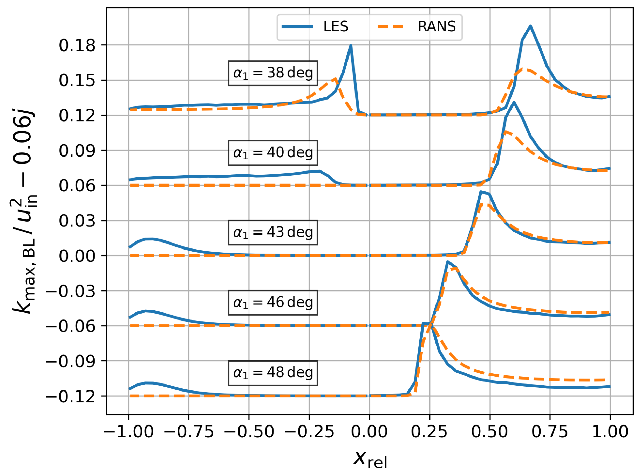
To shed more light on the transition of the boundary layer, the maximum turbulent kinetic energy along several boundary layer cuts on the suction and pressure side is shown in Figure 13. The differences on the pressure side are most obvious. One can confirm the observation made in the analysis of the skin friction coefficient that, for an inflow angle of 38 deg , RANS predicts a significantly delayed transition. Similarly, the transition observed in the LES at 40 deg is not seen in RANS, which features a fully-attached laminar boundary layer. Interesting observations can also be made close to the TE, where low-frequency oscillations occur for α 1 43 deg . Certainly, these are not transition effects in the attached boundary layer but rather oscillations of large-scale structures forming due to the profile shape. In Figure 9-D, their effect on the wake is also visible in the instantaneous flow field.
On the suction side, the differences between RANS and LES are the largest in the negative incidence cases. While the transition onset agrees fairly well, the level of turbulent kinetic energy behind reattachment differs significantly. With increased incidence angles, the differences in the level of turbulent kinetic energy reduce. It is, however, notable that, for positive incidence angles, RANS features a higher turbulent kinetic energy after transition, which seems to contradict the friction coefficient distribution in Figure 12. However, when examining the 2D distribution of turbulent kinetic energy along the boundary layer, as shown in Figure 14, the maximum is closer to the wall in the LES. With approximately equal displacement thicknesses, the RANS exhibits a higher boundary layer momentum thickness compared to the LES, resulting in larger shape factors and a reduced skin friction beyond the transition region on the suction side.

4.5. Conventional Wake Loss Analysis

An important design quantity is the profile loss coefficient. While there are multiple definitions of the loss, typically, the total pressure loss is measured and investigated with the experiments [40]. Following Equation (5), the total pressure loss of the experiment, RANS and LES for the considered inflow angles is shown in Figure 15.
The LES and experimental results agree exceptionally well in terms of both wake width and peak loss, except for the 48 deg case. Only the loss profile of this high-incidence case exhibits notable discrepancies. The experiment shows higher total pressure loss on the suction side as the wake width increases, which is surprising since the isentropic Mach number distribution on the suction side aligns well with the LES, cf. Figure 11. Possible reasons for this discrepancy could be on both sides. On the one hand, inhomogeneous (in-)flow conditions might affect the results of the experiment, leading to certain blades being more heavily loaded. The experiment also exhibits total pressure loss in the suction side passage, which is found neither on the pressure side of the experiment, nor on the pressure and suction side passage in the RANS and LES results. On the other hand, although carefully set up, the LES might also exhibit some uncertainties. However, a simulation with two blades, i.e., the setup has been duplicated in the pitchwise direction, showed no effect on the total pressure loss. Furthermore, significant under-resolution of the LES is considered as rather unlikely, since virtually no turbulent structures propagate into the coarser wake region. On the chosen resolution, a grid convergence index of 0.40 % for the integral loss of the 48 deg case is reached. Additionally, a high-order spatial discretization is employed, which is known for its excellent dispersion and dissipation properties, even at coarse grid resolutions [41]. A simulation with an extended structured zone around the blade and a refined outer wake region, totaling 7.0 × 10 6 DOF, affirms that there is virtually no difference in the total pressure loss.
Comparing RANS with both other results, large discrepancies, especially in the peak loss, can be observed, which is a known issue for RANS at lower Reynolds numbers, cf. [42,43,44]. For the positive incidence angles, the pressure side branch of the wake loss aligns well with the LES. Yet, the width towards the suction side is overestimated. This effect could be related to the larger momentum thickness and more energetic boundary layer, as discussed in the previous section, which was especially present in the positive incidence case, cf. Figure 14. At negative incidence angles, the flank on the pressure side diverges from those found in the LES and experiment, which could be linked to the discrepancies found in the separation and transition behavior. In contrast, the position of the wake loss profile on the suction side is well aligned across all three results for negative incidence angles. However, RANS consistently shows a significantly higher peak loss.
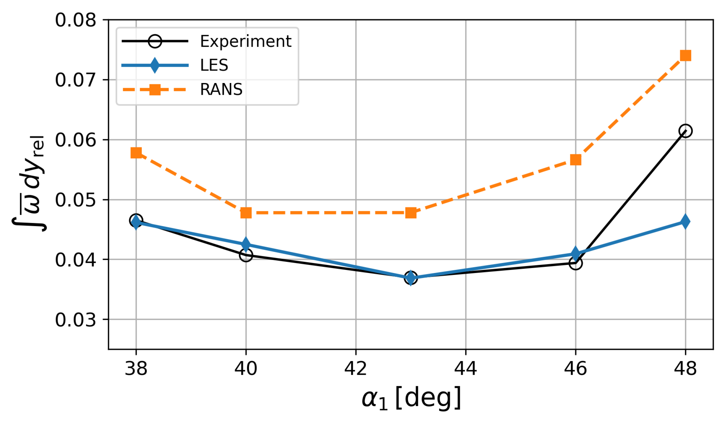
In profile design optimizations, the shape of the loss profile is often irrelevant and only the integrated loss coefficient is considered. For this, flux-averaged or mixed-out quantities are analyzed. However, for the present experimental campaign, the definition of mixed-out quantities could not be comprehensively applied to the RANS and LES data. Since the mass flow distribution was not available over the MP2 of the experiment but all methodologies share the same position of MP2, we directly compare the area-integrated total pressure loss coefficient, acknowledging that the physical foundation of an area-averaged stagnation pressure is not given [45]. Figure 16 shows the respective loss polars for RANS, LES and the experiments. RANS shows the expected offset. The largest difference of 43.7 % is found to be with α 1 = 46 deg , see Table 4. Apart from the highest incidence case, in which elevated loss levels also occur in the passage, the LES agrees very well with the experiment, exhibiting relative differences below 5 % .
Another important observation can be made here. RANS shows a disagreement regarding the optimal incidence angle compared to the findings from the LES and experimental results. Specifically, while the optimal inflow angle is identified as 43 deg for both the LES and the experiment, RANS does not align with this value. In traditional design paradigms, the primary focus is often on the general trend of the results rather than exact values. If the trend predicted by the model is correct, a small offset of loss in the optimal angle might be acceptable. However, in this case, the discrepancy in the optimal incidence angle represents a substantial issue. This deviation suggests that RANS does not accurately capture crucial aspects of the profile behavior for flows with low Reynolds numbers, which could impact the design and performance predictions.

4.6. Cascade Deflection Characteristics

Figure 17 shows the deflection characteristics of the cascade for the different inflow angles. It is computed as
δ = α 1 arctan v ¯ u ¯ .
Clearly, the agreement between the experiment and LES is improved compared to RANS for this quantity, with a maximum difference of 0.68 deg. RANS shows a larger deviation from the experiment over the whole working range, underestimating the cascade deflection by about 2.4 deg at maximum. While this may not seem significant at first glance, in profile design optimization, where flow deflection is often a restrictive constraint, the converged optimization results can fall outside the design constraints when re-evaluated with high-fidelity approaches or experiments. For the positive-incidence off-design point, both numerical deflection characteristics deviate from the experiment, which is most likely also linked to the increase of loss and uncertainties in the experimental setup observed and discussed in Figure 16.

4.7. Entropy Generation Breakdown

In the previous section, a discrepancy between the profile loss predicted by RANS and LES was identified. In the literature, such discrepancies are often addressed indirectly, for example by analyzing boundary layer development or wake structures. While these approaches can yield useful observations, they typically do not provide a direct link to the underlying loss mechanisms. To enable a more targeted investigation, the present work leverages high-fidelity simulation data in combination with an entropy generation analysis based on the entropy balance equation. This approach, derived and employed for example by Kock et al. [46,47], and more recently adapted for turbomachinery applications [48,49], facilitates a more direct and physically motivated assessment of irreversible losses.
Ignoring the effects of temperature gradients and fluctuations, the main contributions to the Favre-averaged entropy generation are [46]
g s mean = V 1 T ˜ σ i j ˜ u i ˜ x j d V and g s turbulent = V 1 T ˜ σ i j u i x j ¯ d V = V 1 T ˜ ρ ¯ ε d V ,
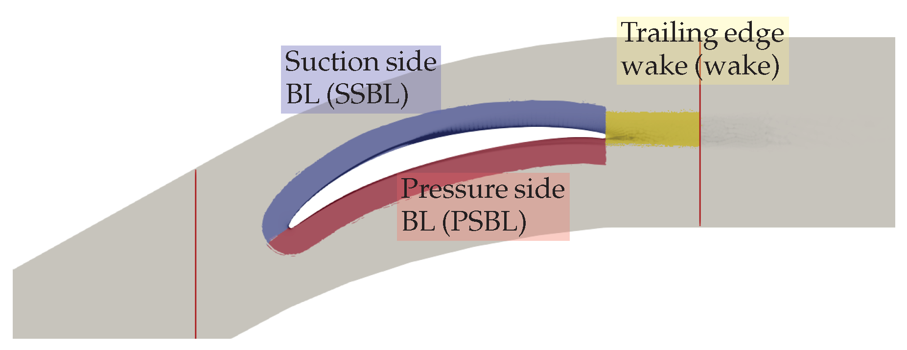
where V is the volume, T ˜ is the Favre-averaged temperature, σ i j is the viscous stress tensor and ρ ¯ ϵ is the Favre-averaged turbulent dissipation rate from the turbulent kinetic energy equation [50]. Equally, one could now replace the turbulent dissipation rate by the balancing terms of the turbulent kinetic energy equation, cf. [48]; however, for the current article, the dissipation is used directly. Note that we only consider the resolved scales in the implicit LES, which is justified considering the high resolution of the present case. Furthermore, a decomposition of the domain into three different zones is performed following Raina et al. [51]:
  • Suction-side boundary layer with d / c 0.1 and above the camber line;
  • Pressure-side boundary layer with d / c 0.1 and below the camber line;
  • Trailing edge wake with ( T ˜ Δ s ˜ u ˜ 2 > 0.01 | ω ˜ z | > | ω ˜ x | | ω ˜ z | > | ω ˜ y | ), where ω ˜ is the vorticity vector and the prime coordinates represent the coordinate system aligned with the mean flow.
The different zones are sketched in Figure 18 for the LES at the ADP.
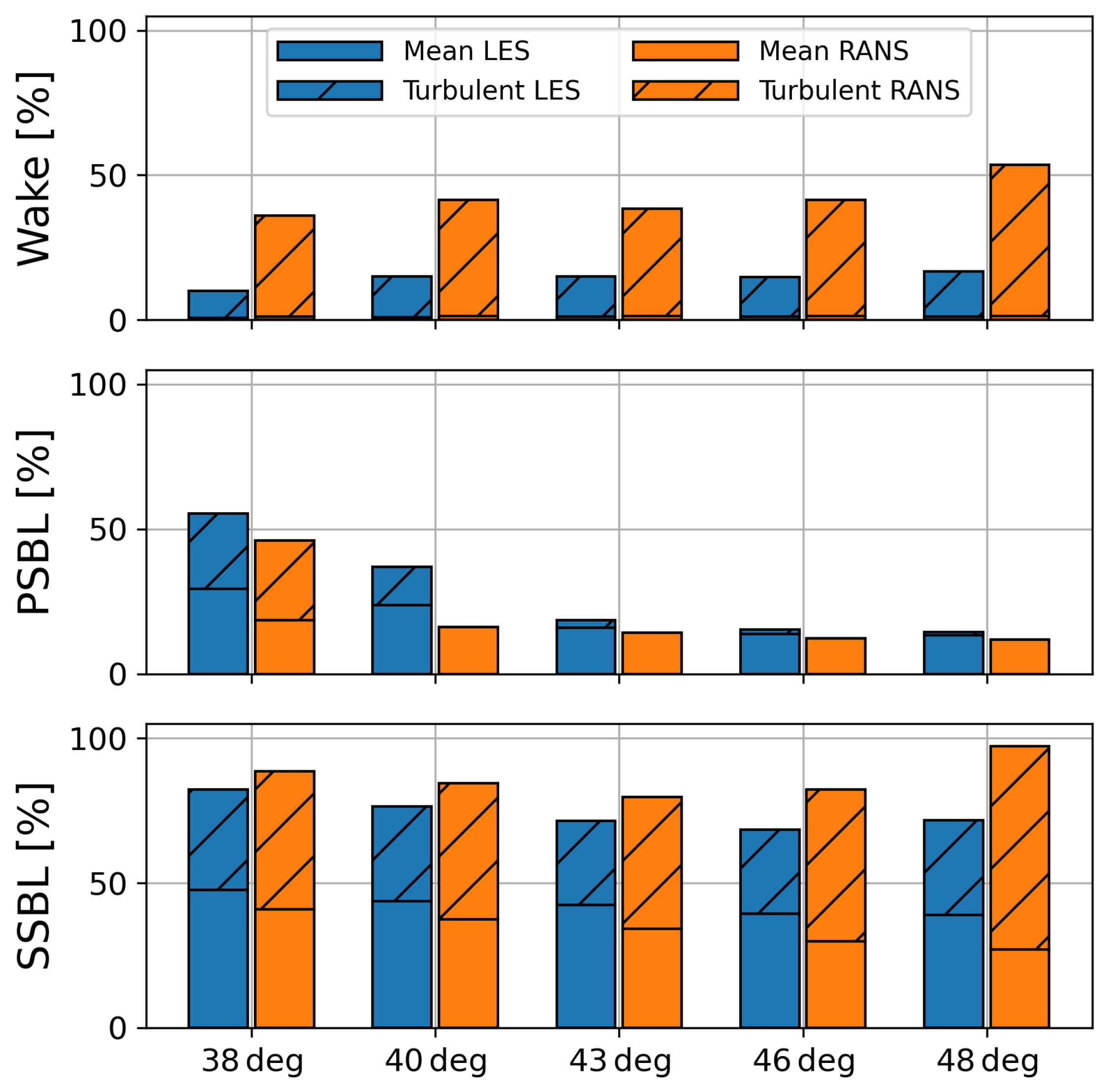
The results of the spatial decomposition of the entropy generation mechanisms normalized with the total entropy generation of the LES in the ADP are shown in Figure 19. Several observations can be made here. The first, which stands out the most, is that RANS overestimates the turbulent dissipation in the wake of the profile for all inflow angles, which can be linked to the overestimation of integral total pressure loss as shown in Figure 16. In the suction-side boundary layer, the agreement is better than in the wake. Nevertheless, the mean flow contributions of RANS for all incidence angles are lower than in LES, which is consistent with the lower skin friction on the suction side observed in Figure 12. The trend of the turbulent contributions follows the observations made in the wake, where the difference is especially pronounced in the highest positive incidence case ( 48 deg ) with the integral turbulent dissipation rate more than doubled for RANS. Combined with the higher entropy generation in the wake, this seems to be a main factor for the large total pressure loss observed in Figure 15. On the pressure side, a transitional boundary layer can be observed for decreasing inflow angles. Here, the turbulent content increases significantly at 40 deg and 38 deg , contributing to the overall entropy generation. In contrast, for RANS, turbulent dissipation is observed at 38 deg but not at 40 deg , highlighting its inability to correctly predict the transition on the pressure side.

5. Conclusions

This paper compares and analyses the effects of different incidence angles on a compressor cascade’s flow parameters, measured and simulated with RANS and LES at a Mach number of 0.6 and a Reynolds number of 150,000. The experimental measurement campaign serves as the foundation of the analysis, providing the in- and outflow boundary conditions as is, without relying on artificial tuning. In particular, note that the same turbulent decay was used for the RANS and the LES.
The analysis of the high-fidelity setup reveals the significant influence of the AVDR and the inflow turbulence. Ignoring the AVDR certainly results in a different flow topology, shifting the total pressure loss towards the suction side. The influence of the inflow turbulence was surprising since the turbulence intensity is only about 0.3 % . Yet, the laminar separation bubble was found to be susceptible to the perturbations that reduce its length by 29 % .
The findings from the study with five inflow angles can be summarized as follows. The agreement of the experiment and the LES is remarkable for the isentropic Mach number distribution and total pressure loss coefficients. Noticeable differences can only be found for the high positive incidence angle, where the loss on the suction side is higher than in the experiment. The accuracy of RANS with the γ - Re θ transition model for the presented cases is also considerable. Major effects can be quite well predicted, e.g., the shift of the suction-side separation and transition towards the leading edge for higher inflow angles or the transition occurring on the pressure side for the high negative incidence case with α 1 = 38 deg . Nevertheless, deviations are still present, which can even negatively influence design decisions. Generally, RANS showed a significant deviation in the integral total pressure loss compared to the experimental results of at least 17.3 % but up to 41.1 % . While a constant offset might be tolerable, trends should be correct. In contrast to the experiment and to the LES, the least integral loss was not predicted in the ADP but at an inflow angle of 40 deg , i.e., 2 deg incidence. Based on the comparison with LES in the form of boundary layer analysis and entropy generation breakdown, this was linked to a failure to predict transition on the pressure side of the cascade and, hence, missing entropy generation from the turbulent boundary layer. In addition, our analysis revealed that TKE profiles in the suction-side boundary layer were thicker in RANS, i.e., having a larger momentum thickness compared to LES for all inflow angles and, therefore, larger suction-side boundary layer loss. Moreover, the turbulent contribution to the generation inside the wake is also over-predicted by RANS for all incidence angles, which translates to the larger integral total pressure loss coefficient.
To conclude, the high-fidelity simulations using TRACE’s DG solver demonstrate experimental-like accuracy for the considered compressor cascade flows in low-Reynolds-number conditions. The detailed data provided by LES allow for an in-depth analysis of the differences compared to RANS, revealing the limitations of the latter in predicting certain flow characteristics in these off-design conditions.
While it is difficult to establish a general guideline for designers based on this study, the main takeaway is that the uncertainties introduced by RANS do not always result in a constant offset over the working range but are flow dependent and especially pronounced in off-design conditions with an expected impact on working range predictions [52]. This might lead to finding sub-optimal designs, which might even violate design constraints when being re-evaluated with experiments. With the increasing feasibility of high-fidelity scale-resolving simulations, particularly for low Reynolds number flows, LES offers a powerful tool for validating design predictions early in the development process. One step forward could be to adjust optimization constraints or targets based on the differences between LES and RANS for the baseline design. In future studies, we aim to leverage the high accuracy of LES in automated design optimization procedures, increasing fidelity levels and improving predictive capabilities at challenging operating points. This approach has the potential to enhance design reliability and reduce the reliance on experimental validation in early-stage development.

Supplementary Materials

The following supporting information can be downloaded at: https://www.mdpi.com/article/10.3390/ijtpp10040042/s1, Video S1: Instantaneous flow field visualization from the LES for the five considered operating points. The five LES results were superimposed a posteriori in a single video.

Author Contributions

Conceptualization, M.B. and F.M.M.; methodology, M.B., C.M. and F.M.M.; software, M.B. and B.F.K.; validation, M.B. and F.M.M.; formal analysis, M.B.; investigation, M.B., F.M.M. and A.H.; data curation, M.B. and F.M.M.; writing—original draft preparation, M.B.; writing—review and editing, M.B., C.M., F.M.M., B.F.K., A.H. and G.G.; visualization, M.B.; project administration, M.B. and G.G.; funding acquisition, M.B., C.M., A.H. and G.G. All authors have read and agreed to the published version of the manuscript.

Funding

Michael Bergmann and Georgios Goinis would like to thank the European Union for funding their research under grant number 101138080 (Project Sci-Fi-Turbo). The views and opinions expressed are, however, those of the author(s) only and do not necessarily reflect those of the European Union. Neither the European Union nor the granting authority can be held responsible for them.

Institutional Review Board Statement

Not applicable.

Informed Consent Statement

Not applicable.

Data Availability Statement

The data presented in this study are available upon request from the corresponding author.

Acknowledgments

The authors gratefully acknowledge the scientific support and HPC resources provided by the German Aerospace Center (DLR). All simulations in this work have been carried out on the HPC system CARA, which is partially funded by ‘Saxon State Ministry for Economic Affairs, Labour and Transport’ and ‘Federal Ministry for Economic Affairs and Climate Action’.

Conflicts of Interest

The authors declare no conflicts of interest.

Abbreviations

The following abbreviations are used in this manuscript:
ADPAerodynamic design point
AVDRAxial velocity density ratio
DGDiscontinuous Galerkin
DGSEMDiscontinuous Galerkin Spectral Element Method
DOFDegrees of freedom
DNSDirect numerical simulation
LELeading edge
LESLarge-eddy simulation
MPMeasurement plane
MUSCLMonotonic Upstream-centered Scheme for Conservation Laws
RANSReynolds-averaged Navier–Stokes
TETrailing edge
Variables
bPitch
cChord length
c f Skin friction coefficient
dDistance
f s Sampling frequency
gEntropy generation
hChannel height
jIncidence
kTurbulent kinetic energy
pStatic pressure
t c Convective time unit
u in Reference velocity magnitude
x , y , z Cartesian coordinates
FPhysical flux
TStatic temperature
VVolume
MaMach number
ReReynolds number
TuTurbulence intensity
α Angle
δ Deflection angle
ϵ Turbulent dissipation rate
ρ in Reference density
ω Total pressure loss, vorticity
σ Viscous stress
ξ , η , ζ Blade-aligned directions (streamwise, normal, spanwise)
Subscripts
1Inflow conditions at MP1
2Outflow conditions at MP2
inConditions at CFD inlet
outConditions at CFD outlet
tStagnation-point values
sStagger angle
advAdvective component
relRelative

References

  1. Hergt, A.; Pesch, M.; Grund, S.; Flamm, J. Low Reynolds Number Effects in Compressor Blade Design. Int. J. Gas Turbine Propuls. Power Syst. 2024, 15, v15n4tp08. [Google Scholar] [CrossRef]
  2. Diehl, M.; Schreiber, C.; Schiffmann, J. The Role of Reynolds Number Effect and Tip Leakage in Compressor Geometry Scaling at Low Turbulent Reynolds Numbers. J. Turbomach. 2020, 142, 031003. [Google Scholar] [CrossRef]
  3. Bennett, M.; Chapman, J.W.; Wells, D.P. An Approach to Evaluating the Impact of Small-core Turbofan Technologies on Engine and Aircraft Performance. In Proceedings of the AIAA SCITECH 2024 Forum, Orlando, FL, USA, 8–12 January 2024. [Google Scholar] [CrossRef]
  4. Voß, C.; Aulich, M.; Kaplan, B.; Nicke, E. Automated Multiobjective Optimisation in Axial Compressor Blade Design. In Proceedings of the ASME Turbo Expo: Power for Land, Sea, and Air, Barcelona, Spain, 8–11 May 2006; Volume 6: Turbomachinery, Parts A and B, pp. 1289–1297. [Google Scholar] [CrossRef]
  5. Voß, C.; Hemmert-Pottmann, S.; Schmitz, A. Multi-fidelity optimization of a highly loaded low pressure compressor. In Proceedings of the Second European Workshop on MDO for Aeronautical Industrial Applications, Toulouse, France, 19–20 November 2019. [Google Scholar]
  6. Michelassi, V.; Chen, L.W.; Pichler, R.; Sandberg, R.D. Compressible Direct Numerical Simulation of Low-Pressure Turbines—Part II: Effect of Inflow Disturbances. J. Turbomach. 2015, 137, 071005. [Google Scholar] [CrossRef]
  7. Leggett, J.; Priebe, S.; Shabbir, A.; Michelassi, V.; Sandberg, R.; Richardson, E. Loss Prediction in an Axial Compressor Cascade at Off-Design Incidences with Free Stream Disturbances Using Large Eddy Simulation. J. Turbomach. 2018, 140, 071005. [Google Scholar] [CrossRef]
  8. Bergmann, M.; Morsbach, C.; Klose, B.F.; Ashcroft, G.; Kügeler, E. A Numerical Test Rig for Turbomachinery Flows Based on Large Eddy Simulations with a High-Order Discontinuous Galerkin Scheme—Part I: Sliding Interfaces and Unsteady Row Interactions. J. Turbomach. 2023, 146, 021005. [Google Scholar] [CrossRef]
  9. Morsbach, C.; Bergmann, M.; Tosun, A.; Klose, B.F.; Bechlars, P.; Kügeler, E. A Numerical Test Rig for Turbomachinery Flows Based on Large Eddy Simulations with a High-Order Discontinuous Galerkin Scheme—Part III: Secondary Flow Effects. J. Turbomach. 2023, 146, 021007. [Google Scholar] [CrossRef]
  10. Klose, B.F.; Morsbach, C.; Bergmann, M.; Munoz Lopez, E.J.; Hergt, A.; Kügeler, E. The Unsteady Shock–Boundary Layer Interaction in a Compressor Cascade—Part II: High-Fidelity Simulation. J. Turbomach. 2025, 147, 091002. [Google Scholar] [CrossRef]
  11. Choi, H.; Moin, P. Grid-point requirements for large eddy simulation: Chapman’s estimates revisited. Phys. Fluids 2012, 24, 011702. [Google Scholar] [CrossRef]
  12. Bergmann, M.; Gölden, R.; Morsbach, C. Numerical investigation of split form nodal discontinuous Galerkin schemes for the implicit LES of a turbulent channel flow. In Proceedings of the 7th European Conference on Computational Fluid Dynamics, Glasgow, UK, 11–15 June 2018. [Google Scholar]
  13. Bergmann, M. A Split-Form Discontinuous Galerkin Spectral Element Framework for Scale-Resolving Simulations of Turbomachinery Flows. Ph.D. Thesis, Universitätsbibliothek, Ruhr-Universität Bochum, Bochum, Germany, 2024. [Google Scholar] [CrossRef]
  14. Bergmann, M.; Morsbach, C.; Ashcroft, G. Assessment of Split Form Nodal Discontinuous Galerkin Schemes for the LES of a Low Pressure Turbine Profile. In Proceedings of the Direct and Large Eddy Simulation XII, Madrid, Spain, 5–7 June 2019; García-Villalba, M., Kuerten, H., Salvetti, M.V., Eds.; Springer: Cham, Switzerland, 2020; pp. 365–371. [Google Scholar]
  15. Klose, B.F.; Morsbach, C.; Bergmann, M.; Hergt, A.; Klinner, J.; Grund, S.; Kügeler, E. A Numerical Test Rig for Turbomachinery Flows Based on Large Eddy Simulations with a High-Order Discontinuous Galerkin Scheme—Part II: Shock Capturing and Transonic Flows. J. Turbomach. 2023, 146, 021006. [Google Scholar] [CrossRef]
  16. Bergmann, M.; Morsbach, C.; Möller, F.M.; Klose, B.F.; Hergt, A.; Goinis, G. A Comparative Study of Varying Incidence Angle Effects on a Low-Reynolds-Number Compressor Cascade Based on Experiments and Low-Fidelity and High-Fidelity Numerical Simulations. In Proceedings of the 16th European Turbomachinery Conference, Paper n. ETC2025-231. Hannover, Germany, 24–28 March 2025. [Google Scholar]
  17. Sonoda, T.; Yamaguchi, Y.; Arima, T.; Olhofer, M.; Sendhoff, B.; Schreiber, H.A. Advanced High Turning Compressor Airfoils for Low Reynolds Number Condition—Part I: Design and Optimization. J. Turbomach. 2004, 126, 350–359. [Google Scholar] [CrossRef]
  18. Schreiber, H.A.; Steinert, W.; Sonoda, T.; Arima, T. Advanced High-Turning Compressor Airfoils for Low Reynolds Number Condition—Part II: Experimental and Numerical Analysis. J. Turbomach. 2004, 126, 482–492. [Google Scholar] [CrossRef]
  19. Hergt, A.; Hage, W.; Grund, S.; Steinert, W.; Terhorst, M.; Schongen, F.; Wilke, Y. Riblet Application in Compressors: Toward Efficient Blade Design. J. Turbomach. 2015, 137, 111006. [Google Scholar] [CrossRef]
  20. Steinert, W.; Fuchs, R.; Starken, H. Inlet Flow Angle Determination of Transonic Compressor Cascades. J. Turbomach. 1992, 114, 487–493. [Google Scholar] [CrossRef]
  21. Hergt, A.; Klinner, J.; Grund, S.; Willert, C.; Steinert, W.; Beversdorff, M. On the Importance of Transition Control at Transonic Compressor Blades. J. Turbomach. 2021, 143, 031007. [Google Scholar] [CrossRef]
  22. Morsbach, C.; di Mare, F. Conservative segregated solution method for turbulence model equations in compressible flows. In Proceedings of the 6th European Congress on Computational Methods in Applied Sciences and Engineering (ECCOMAS 2012), Vienna, Austria, 10–14 September 2012. [Google Scholar]
  23. Menter, F.; Kuntz, M.; Langtry, R. Ten years of Industrial experience with the SST model. In Proceedings of the Turbulence, Heat and Mass Transfer 4, Antalya, Turkey, 12–17 October 2003; Hanjalić, K., Nagano, Y., Tummers, M., Eds.; Begell House, Inc.: Danbury, CT, USA, 2003; pp. 625–632. [Google Scholar]
  24. Kato, M.; Launder, B.E. The Modeling of Turbulent Flow Around Stationary and Vibrating Square Cylinders. In Proceedings of the 9th Symposium on Turbulent Shear Flows, Kyoto, Japan, 16–18 August 1993; pp. 10.4.1–10.4.6. [Google Scholar]
  25. Langtry, R.B.; Menter, F.R. Correlation-Based Transition Modeling for Unstructured Parallelized Computational Fluid Dynamics Codes. AIAA J. 2009, 47, 2894–2906. [Google Scholar] [CrossRef]
  26. Schlüß, D.; Frey, C.; Ashcroft, G. Consistent Non-reflecting Boundary Conditions for Both Steady and Unsteady Flow Simulations in Turbomachinery Applications. In Proceedings of the ECCOMAS Congress 2016 VII European Congress on Computational Methods in Applied Sciences and Engineering, Crete, Greece, 5–10 June 2016. [Google Scholar]
  27. Giles, M. UNSFLO: A Numerical Method for the Calculation of Unsteady Flow in Turobmachinery; Technical report, Gas Turbine Laboratory Report GTL 205; MIT Department of Aeronautics and Astronautics: Cambridge, MA, USA, 1991. [Google Scholar]
  28. Bolinches-Gisbert, M.; Robles, D.C.; Corral, R.; Gisbert, F. Prediction of Reynolds Number Effects on Low-Pressure Turbines Using a High-Order ILES Method. J. Turbomach. 2020, 142, 031002. [Google Scholar] [CrossRef]
  29. Weber, A.; Sauer, M. PyMesh—Template Documentation; Technical report DLR-IB-AT-KP-2016-34; Institute of Propulsion Technology, German Aerospace Center (DLR): Cologne, Germany, 2016. [Google Scholar]
  30. Bassi, F.; Rebay, S. A High-Order Accurate Discontinuous Finite Element Method for the Numerical Solution of the Compressible Navier–Stokes Equations. J. Comput. Phys. 1997, 131, 267–279. [Google Scholar] [CrossRef]
  31. Gassner, G.J.; Winters, A.R.; Kopriva, D.A. Split form nodal discontinuous Galerkin schemes with summation-by-parts property for the compressible Euler equations. J. Comput. Phys. 2016, 327, 39–66. [Google Scholar] [CrossRef]
  32. Kennedy, C.A.; Gruber, A. Reduced Aliasing Formulations of the Convective Terms Within the Navier-Stokes Equations for a Compressible Fluid. J. Comput. Phys. 2008, 227, 1676–1700. [Google Scholar] [CrossRef]
  33. Shu, C.W.; Osher, S. Efficient implementation of essentially non-oscillatory shock-capturing schemes. J. Comput. Phys. 1988, 77, 439–471. [Google Scholar] [CrossRef]
  34. Shur, M.L.; Spalart, P.R.; Strelets, M.K.; Travin, A.K. Synthetic Turbulence Generators for RANS-LES Interfaces in Zonal Simulations of Aerodynamic and Aeroacoustic Problems. Flow Turbul. Combus. 2014, 93, 63–92. [Google Scholar] [CrossRef]
  35. Morsbach, C.; Franke, M. Analysis of a Synthetic Turbulence Generation Method for Periodic Configurations. In Proceedings of the Direct and Large-Eddy Simulation XI; Salvetti, M.V., Armenio, V., Fröhlich, J., Geurts, B.J., Kuerten, H., Eds.; Springer: Cham, Switzerland, 2019; pp. 169–174. [Google Scholar]
  36. Leyh, S.; Morsbach, C. The Coupling of a Synthetic Turbulence Generator with Turbomachinery Boundary Conditions. In Proceedings of the Direct and Large Eddy Simulation XII; García-Villalba, M., Kuerten, H., Salvetti, M.V., Eds.; Springer: Cham, Switzerland, 2020. [Google Scholar]
  37. Geuzaine, C.; Remacle, J.F. Gmsh: A 3-D finite element mesh generator with built-in pre- and post-processing facilities. Int. J. Numer. Methods Eng. 2009, 79, 1309–1331. [Google Scholar] [CrossRef]
  38. Georgiadis, N.J.; Rizzetta, D.P.; Fureby, C. Large-Eddy Simulation: Current Capabilities, Recommended Practices, and Future Research. AIAA J. 2012, 48, 1772–1784. [Google Scholar] [CrossRef]
  39. Bergmann, M.; Morsbach, C.; Ashcroft, G.; Kügeler, E. Statistical Error Estimation Methods for Engineering-Relevant Quantities From Scale-Resolving Simulations. J. Turbomach. 2021, 144, 031005. [Google Scholar] [CrossRef]
  40. Denton, J.D. Loss Mechanisms in Turbomachines. In Proceedings of the ASME 1993 International Gas Turbine and Aeroengine Congress and Exposition, Cincinnati, OH, USA, 24–27 May 1993; Volume 2: Combustion and Fuels; Oil and Gas Applications; Cycle Innovations; Heat Transfer; Electric Power; Industrial and Cogeneration; Ceramics; Structures and Dynamics; Controls, Diagnostics and Instrumentation. [Google Scholar] [CrossRef]
  41. Gassner, G.J.; Beck, A.D. On the accuracy of high-order discretizations for underresolved turbulence simulations. Theor. Comput. Fluid Dyn. 2012, 27, 221–237. [Google Scholar] [CrossRef]
  42. Muth, B.; Schwarze, M.; Niehuis, R.; Franke, M. Investigation of CFD Prediction Capabilities for Low Reynolds Turbine Aerodynamics. In Proceedings of the ASME Turbo Expo 2009: Power for Land, Sea, and Air, Orlando, FL, USA, 8–12 June 2009; ASMEDC: New York, NY, USA, 2009; Volume 7: Turbomachinery, Parts A and B, pp. 875–884. [Google Scholar] [CrossRef]
  43. Müller-Schindewolffs, C.; Baier, R.D.; Seume, J.R.; Herbst, F. Direct Numerical Simulation Based Analysis of RANS Predictions of a Low-Pressure Turbine Cascade. J. Turbomach. 2017, 139, 081006. [Google Scholar] [CrossRef]
  44. Morsbach, C.; Bergmann, M.; Tosun, A.; Klose, B.F.; Kügeler, E.; Franke, M. Large Eddy Simulation of a Low-Pressure Turbine Cascade with Turbulent End Wall Boundary Layers. Flow Turbul. Combust. 2024, 112, 165–190. [Google Scholar] [CrossRef]
  45. Cumpsty, N.A.; Horlock, J.H. Averaging Nonuniform Flow for a Purpose. J. Turbomach. 2005, 128, 120–129. [Google Scholar] [CrossRef]
  46. Kock, F. Bestimmung der Lokalen Entropieproduktion in Turbulenten Strömungen und Deren Nutzung zur Bewertung Konvektiver Transportprozesse. Ph.D. Thesis, TU Hamburg-Harburg, Hamburg, Germany, 2003. [Google Scholar]
  47. Kock, F.; Herwig, H. Local entropy production in turbulent shear flows: A high-Reynolds number model with wall functions. Int. J. Heat Mass Transf. 2004, 47, 2205–2215. [Google Scholar] [CrossRef]
  48. Zhao, Y.; Sandberg, R.D. Using a New Entropy Loss Analysis to Assess the Accuracy of RANS Predictions of an HPT Vane. In Proceedings of the ASME Turbo Expo 2019: Turbomachinery Technical Conference and Exposition, Phoenix, AZ, USA, 17–21 June 2019; Volume 2C: Turbomachinery. [Google Scholar] [CrossRef]
  49. Borcherding, T.; Bode, C.; Rosenzweig, M.; Przytarski, P.J.; Leggett, J.; Sandberg, R.D. Entropy Loss Breakdown Comparison for LES and RANS of a Transonic Compressor Stage Midspan Section. In Proceedings of the ASME Turbo Expo 2023: Turbomachinery Technical Conference and Exposition, Boston, MA, USA, 26–30 June 2023; Volume 13A: Turbomachinery—Axial Flow Fan and Compressor Aerodynamics. [Google Scholar] [CrossRef]
  50. Wilcox, D. Turbulence Modeling for CFD; Number Bd. 1 in Turbulence Modeling for CFD; DCW Industries: Dhrangadhra, Gujarat, 2006. [Google Scholar]
  51. Raina, G.; Bousquet, Y.; Luquet, D.; Lippinois, E.; Binder, N. Loss Breakdown in Axial Turbines: A New Method for Vortex Loss and Wake Detection from 3D RANS Simulations. J. Turbomach. 2025, 147, 061006. [Google Scholar] [CrossRef]
  52. Goinis, G.; Satcunanathan, S.; Bergmann, M. Examining the Potential of High-Order SRS to Support RANS-Based Compressor Airfoil Optimization. In Proceedings of the ASME Turbo Expo 2025: Turbomachinery Technical Conference and Exposition, Memphis, TN, USA, 16–20 June 2025; Volume 11: Turbomachinery—Deposition, Erosion, Fouling, and Icing; Design Methods & CFD Modeling for Turbomachinery; Ducts, Noise & Component Interactions. [Google Scholar] [CrossRef]
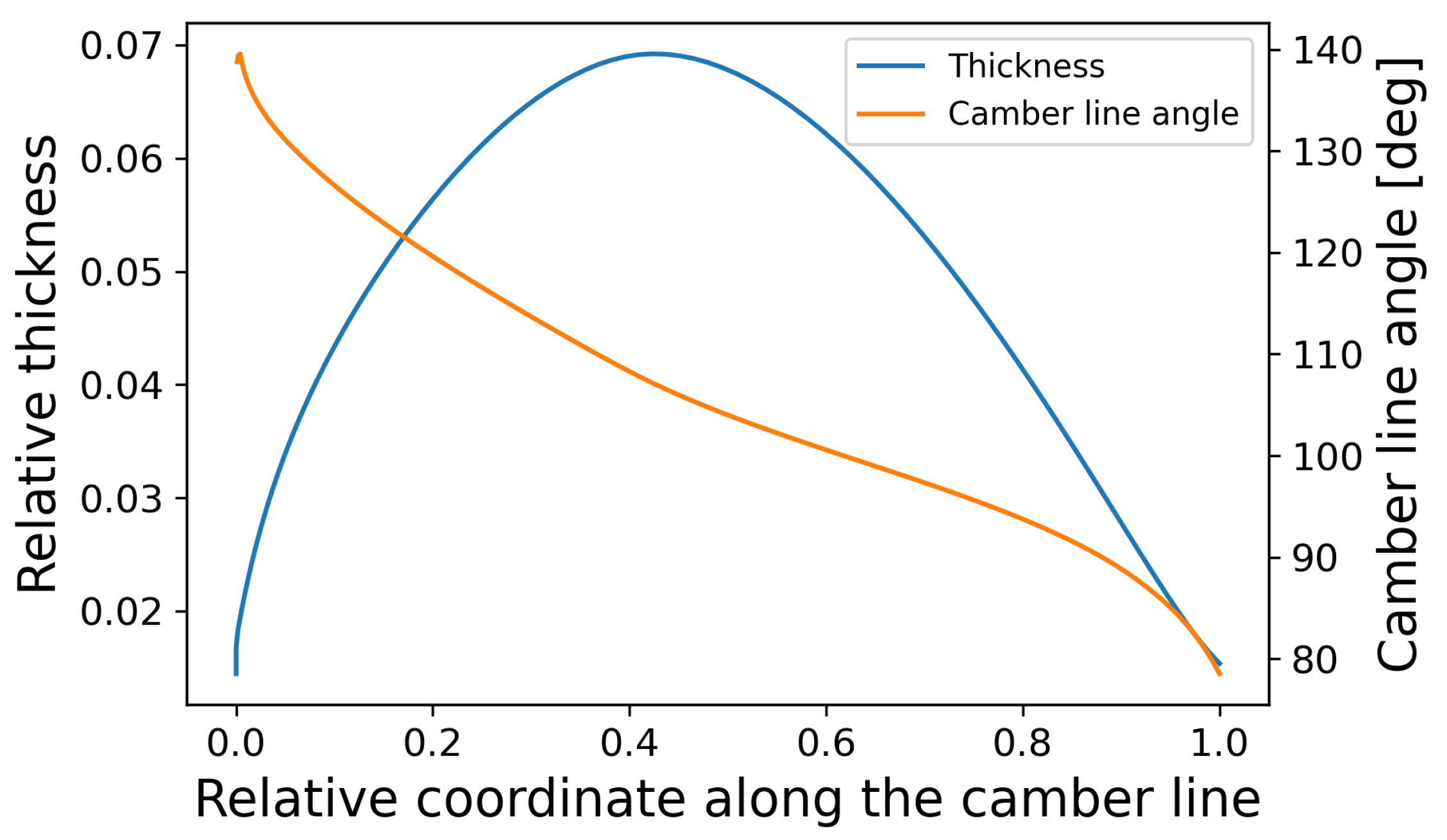
Figure 1. Profile thickness divided by the chord length and camber line angle.
Ijtpp 10 00042 g001
Figure 2. DLR’s Transonic cascade wind tunnel.
Ijtpp 10 00042 g002
Figure 3. RANS and LES domain and mesh in the x-y plane. For the LES, only the high-order grid cells are shown; the solution nodes, i.e., 25 in each 2D element, are omitted for better visibility.
Ijtpp 10 00042 g003
Figure 4. Non-dimensional cell sizes at the blade wall for RANS and LES at the aerodynamic design point. ξ is the wall-tangential, η the wall-normal and ζ the spanwise direction. For the LES, cell-sizes are divided by the polynomial degree N. The suction side is represented by positive values of x rel , while negative values represent the pressure side.
Ijtpp 10 00042 g004
Figure 5. Time- and spanwise-averaged isentropic Mach number distribution around the blade.
Ijtpp 10 00042 g005
Figure 6. Time- and spanwise-averaged total pressure loss coefficient at MP2.
Ijtpp 10 00042 g006
Figure 7. Turbulence intensity Tu along two inflow probes ( α = 43 deg ) for LES-Tu. One probe was directed towards the leading edge and the other one has been moved by a half pitch towards the mid-passage.
Ijtpp 10 00042 g007
Figure 8. Instantaneous flow field on the suction side of the blades of LES-AVDR and LES-Tu. Q-isosurfaces colored by the velocity magnitude are shown in the volume and shear stress wall at the blade wall. Markers A and B denote the reference points discussed in the text.
Ijtpp 10 00042 g008
Figure 9. Instantaneous flow field at the mid span of the LES. The spanwise vorticity normalized by the chord length and mean inflow velocity magnitude of the ADP is shown. The colormap ranges from 26.3 (blue) to 26.3 (red). The illustrated pitch does not represent the original spacing used in the simulations but is reduced for a better visibility. Markers A–D denote the reference points discussed in the text.
Ijtpp 10 00042 g009
Figure 10. Isosurfaces of the Q-criterion coloured by the velocity magnitude on the blade’s pressure side of the LES with α 1 = 38 deg and α 1 = 40 deg . Markers A–C denote the reference points discussed in the text.
Ijtpp 10 00042 g010
Figure 11. Isentropic Mach number distribution along the blade for different inflow angles.
Ijtpp 10 00042 g011
Figure 12. Time- and space-averaged skin friction coefficient along the blade for different inflow angles. The suction side is represented by positive values of x rel , while the pressure side is represented by negative values.
Ijtpp 10 00042 g012
Figure 13. Maximum turbulent kinetic energy k max , BL along boundary layer cuts on the suction ( + x rel ) and the pressure ( x rel ) side. The position of the root point of the boundary layer cut on the blade surface determines the x value in the plot. The turbulent kinetic energy is normalized by the squared mean inflow velocity u in 2 .
Ijtpp 10 00042 g013
Figure 14. Turbulent kinetic energy k distribution along boundary layer cuts on the suction ( + x rel ) and the pressure ( x rel ) side. The y-axis of each subplot represents the normalized wall distance. The results of LES are shown as colored contours and the RANS results as white dotted contour lines.
Ijtpp 10 00042 g014
Figure 15. Time- and space-averaged total pressure loss coefficient ω ¯ along the normalized pitchwise coordinate y rel of MP2.
Ijtpp 10 00042 g015
Figure 16. Pitchwise-integrated total pressure loss coefficient on MP2.
Ijtpp 10 00042 g016
Figure 17. Pitchwise-integrated deflection angle δ at MP2.
Ijtpp 10 00042 g017
Figure 18. Zones of the entropy generation analysis for the ADP flow field. The total viscous dissipation is sketched in grayscale.
Ijtpp 10 00042 g018
Figure 19. Mean and turbulent entropy generation contributions (Equation (9)) in three regions compared for RANS and LES for the five considered inflow angles α 1 . The results are normalized by the total contribution of the LES in the ADP.
Ijtpp 10 00042 g019
Table 1. Cascade design parameters.
Inflow Mach number Ma 1 0.60
Inflow Reynolds number Re 1 1.5 × 10 5
Inflow angle α 1 43 deg
Inflow turbulence intensity Tu 1 0.5 %
Chord length c70 mm
Pitch to chord ratio b / c 0.577
Height to chord ratio h / c 2.4
Stagger angle α s 16.04 deg
AVDR 1.03
Table 2. Overview of the experimental and simulation setup presented in Section 3.
Ma1Re1α1 [deg]Tu1 [%]LT/cAVDRΔz/cDOF [106]
Experiment0.603150,79143.00.3–0.5-1.03822.4
LES-Base0.630155,37743.00010.263.7
LES-AVDR0.600150,29443.0001.03810.263.7
LES-Span0.40.600150,29743.0001.03800.4127.5
LES-Tu0.603150,83343.00.330.014291.03810.263.7
Table 3. Overview of the experimental and simulation setups presented in Section 4.
Ma1Re1α1 [deg]Tu1 [%]AVDR
α 1 = 38 deg , j = 2
Exp0.603160,36138.00.3–0.51.035
RANS0.598159,29038.00.351.035
LES0.603160,37938.00.351.036
α 1 = 40 deg , j = 1
Exp0.602151,99240.00.3–0.51.024
RANS0.595151,12740.00.361.024
LES0.601151,77340.00.351.024
α 1 = 43 deg , j = 0
Exp0.603150,79143.00.3–0.51.038
RANS0.595149,44343.00.351.038
LES0.603150,83343.00.331.038
α 1 = 46 deg , j = + 1
Exp0.600147,76446.00.3–0.51.032
RANS0.590145,86246.00.351.032
LES0.599147,44646.00.341.032
α 1 = 48 deg , j = + 2
Exp0.593149,44748.00.3–0.51.024
RANS0.593149,25948.00.351.024
LES0.608152,00248.00.381.024
Table 4. Relative difference to the experimental integrated total pressure loss.
38 deg 40 deg 43 deg 46 deg 48 deg
RANS24.0%17.3%29.3%43.7%20.5%
LES−0.8%4.4%−0.3 %3.9%−24.6%
Disclaimer/Publisher’s Note: The statements, opinions and data contained in all publications are solely those of the individual author(s) and contributor(s) and not of MDPI and/or the editor(s). MDPI and/or the editor(s) disclaim responsibility for any injury to people or property resulting from any ideas, methods, instructions or products referred to in the content.