Toward the Detection of Flow Separation for Operating Airfoils Using Machine Learning

Abstract

Turbulent flow separation over lifting surfaces impacts high-lift systems such as aircraft, wind turbines, and turbomachinery, and contributes to noise, lift loss, and vibrations. Accurate detection of flow separation is therefore essential to enable active control strategies and to mitigate its adverse effects. Several machine learning models are compared for detecting flow separation from surface pressure fluctuations. The models were trained on experimental data covering various airfoils, angles of attack (0°–23°), and Reynolds numbers, with ${\mathrm{Re}}_c=0.8–4.5\times {10}^6$. For supervised learning, the ground-truth binary labels (attached or separated flow) were derived from static pressure distributions, lift coefficients, and the power spectral densities of surface pressure fluctuations. Three machine learning techniques (multilayer perceptron, support vector machine, logistic regression) were utilized with fine-tuned hyperparameters. Promising results are obtained, with the support vector machine achieving the highest performance (accuracy 0.985, Matthews correlation coefficient 0.975), comparable to other models, with advantages in runtime and model size. However, most misclassifications occur near separation onset due to gradual transition, suggesting areas for model refinement. Sensitivity to database parameters is discussed alongside flow physics and data quality.

1. Introduction

In aerodynamics, where the flow envelops a lifting surface, flow separation occurs when the angle of attack (AoA) exceeds a certain threshold, causing the boundary layer to separate and diminishing the growth rate of lift as a function of AoA. From an aeroacoustic perspective, flow separation can significantly increase noise emission when flow separation takes place at the trailing edge [1]. In addition, flow separation induces significantly increased wall pressure fluctuations, which may amplify structural vibration of the lifting body and potentially reduce its lifespan. These effects are undesirable yet often unavoidable in operation of, for example, a wind turbine due to sudden changes or local variations in the incoming flow.

In order to find potential indicators of separation, several studies have investigated statistical features of wall pressure and wall shear fluctuations [2,3]. In particular, higher-order moments such as skewness (third-order) and kurtosis (fourth-order) have been applied to characterize the distribution of signals and their deviations from Gaussian behavior. Skewness captures asymmetry in the pressure or shear distributions, while kurtosis emphasizes intermittency and the weight of the distribution tails. These quantities have been shown to correlate with flow separation and reattachment in different configurations, making them attractive as compact statistical descriptors. In this context, Le Floc’h et al. [3] demonstrated that massive flow separation is associated with a dominant contribution from low frequencies in the high-order moments, which highlights their potential for mapping the transition from attached to weakly or largely separated flow.

Moving from a physical point of view toward data-driven analysis, recent studies have increasingly demonstrated the potential of machine learning (ML) techniques for flow separation detection and prediction. For a broad perspective on the topic, Hao et al. [4] provided a comprehensive review of ML as a complementary tool to enhance CFD simulations of flow separation. They discussed applications ranging from turbulence model augmentation to reduced-order modeling and physics-informed networks, emphasizing that while ML has demonstrated improvements in accuracy and efficiency, reliable separation prediction across flow regimes, geometries, and Reynolds numbers remains an open challenge. Beyond detection tasks, Hui et al. [5] developed convolutional neural networks that predict entire pressure distributions on airfoils within seconds and with less than 2% error, demonstrating the promise of ML for real-time aerodynamic surrogate modeling.

Along the same line, Yang et al. [6] applied convolutional neural networks (CNNs) to predict wind turbine airfoil noise from a large, dedicated database of 11,700 airfoil profiles, achieving mean absolute percentage errors below 0.1%. More specifically, Shen et al. [7] showed that Bayesian neural networks trained on RANS data can infer aerodynamic coefficients and separation points from sparse static pressure tap measurements. Their work systematically optimized pressure tap positions and demonstrated that reliable predictions can be achieved even with only two to three sensors, as long as they are located near the leading and trailing edges. While this approach achieved low prediction errors across lift, drag, and separation location, it remains inherently tied to the use of static pressure distributions. Such $C_p$-based methods are effective on airfoils, where separation leaves a distinct plateau signature in the pressure distribution, but they may not be transferable to more generic geometries such as bumps or flat plates, where $C_p$ offers no clear indicator of separation. Similarly, Borup et al. [8] demonstrated that neural networks trained on distributed surface pressure sensors can accurately estimate air data parameters such as angle of attack, sideslip angle, and airspeed on small unmanned aerial vehicles, further underlining the potential of surface-pressure-based ML approaches. These results illustrate how ML methods are increasingly applied not only to aerodynamics but also to aeroacoustics in the context of airfoil design.

Expanding beyond $C_p$ inputs, Barthel and Sapsis [9] combined direct numerical simulation (DNS) data with wavelet transforms and simple neural networks to forecast extreme drag events. By coupling physics-informed preprocessing with data-driven models, they demonstrated improved robustness of forecasts, particularly at longer lead times. Yuan et al. [10] explored quantum support vector machines (qSVMs) for aerodynamic classification tasks. Their results showed a significant performance gain: in binary separation detection, classification accuracy improved from 81.8% with classical SVMs to 90.9% with qSVMs, while in multiclass angle-of-attack classification, the accuracy increased from 67% to 79%. These results highlight the potential of advanced ML paradigms for aerodynamics applications. Complementarily to this, Duraisamy et al. [11] focused on systematic ways to reduce uncertainty in RANS closures using statistical inference and ML. Brunton et al. [12] offered an even broader perspective on machine learning for fluid mechanics, covering methods from reduced-order modeling and feature extraction to flow control and optimization, and highlighting both the promise and the limitations of ML in terms of interpretability and generalizability.

Collectively, these studies demonstrate that ML can be successfully applied to flow separation problems, but they also reveal several limitations. Most efforts remain restricted to two-dimensional airfoils, low-to-moderate Reynolds numbers, and small datasets. Inputs are typically limited to static pressure measurements or simple statistical quantities, and few works systematically compare multiple ML methods. Motivated by these considerations, the present study investigates the use of unsteady surface pressure fluctuations $p^{\prime }$ measured on an airfoil in wind tunnel experiments in the context of an ML framework. To ensure robustness across operating conditions, multiple datasets are considered, spanning variations in airfoil geometry, Reynolds number, and angle of attack. Considering different ML techniques, quantities such as training time, model size, execution time, and prediction accuracy are compared in order to find the most suitable one. In addition to accuracy, sensitivity, specificity, and the Matthews correlation coefficient (MCC) [13] were also used to evaluate the model.

This paper is organized as follows: Section 2 introduces the experimental basis and the statistical evaluation of surface pressure data. It is divided into Section 2.1, which describes the wind tunnel setup and data collection, and Section 2.2, which discusses statistical properties of surface pressure fluctuations, as they provide key indicators for distinguishing between attached and separated flow states. Section 3 presents the machine learning framework, with methods (Section 3.1.1, Section 3.1.2 and Section 3.1.3), data preprocessing (Section 3.2.1 and Section 3.2.2), and evaluation metrics (Section 3.3). Section 4 reports the results. The outcomes of MLP, LR, and SVM are given in Section 4.1, Section 4.2 and Section 4.3, with a comparative assessment in Section 4.4. Finally, Section 5 presents the conclusion and offers an outlook on future work.

2. Experimental Basis and Statistical Evaluation of Surface Pressure Data

This section provides the experimental basis for the study. Section 2.1 describes the wind tunnel setup and the acquisition of the surface pressure data, while Section 2.2 discusses statistical properties of the surface pressure fluctuations.

2.1. Experimental Setup and Data Collection

The data used in this study are based on previous studies by Herr and Suryadi et al. [14,15,16]. The data were obtained experimentally in two different test facilities. These are the aeroacoustic wind tunnel (AWB) operated by DLR Institute of Aerodynamics and Flow Technology and the low-speed wind tunnel (NWB) operated by the German–Dutch Wind Tunnels Foundation. Both facilities are located at DLR Braunschweig. The AWB is an open-jet, closed-circuit aeroacoustic wind tunnel with an open test section and nozzle exit area of $1.2 \mathrm{m}\times 0.8 \mathrm{m}$. The maximum flow velocity at the nozzle exit is $u_{\infty }=65 \mathrm{m}/\mathrm{s}$. The NWB offers the options of an open, closed, or slotted test section with a test section area, or nozzle exit area in the case of an open test section, of $2.8 \mathrm{m}\times 3.25 \mathrm{m}$. For closed or slotted test sections, the maximum flow velocity reaches 90 m/s, and for the open-jet section, 80 m/s. In both facilities, the jet is treated with flow straighteners and turbulence control screens at the nozzle inlet to provide a flat velocity profile and reduce inflow turbulence. For more detailed description of the wind tunnels AWB and NWB, the readers are referred to [17,18].

In total, the datasets from three different wind tunnel models were utilized. These include 2.5D (no change in spanwise direction) and 3D models. The 2.5D wind tunnel models are based on the DU96-W-180 and NACA ${63}_{3}018$ airfoils, for which measurements were carried out in the AWB in an open test section and in the NWB in a closed test section. The 3D model is based on NACA 64-618 [16] and was tested in the NWB using a three-quarter-open test section (with a floor from the nozzle to the collector). 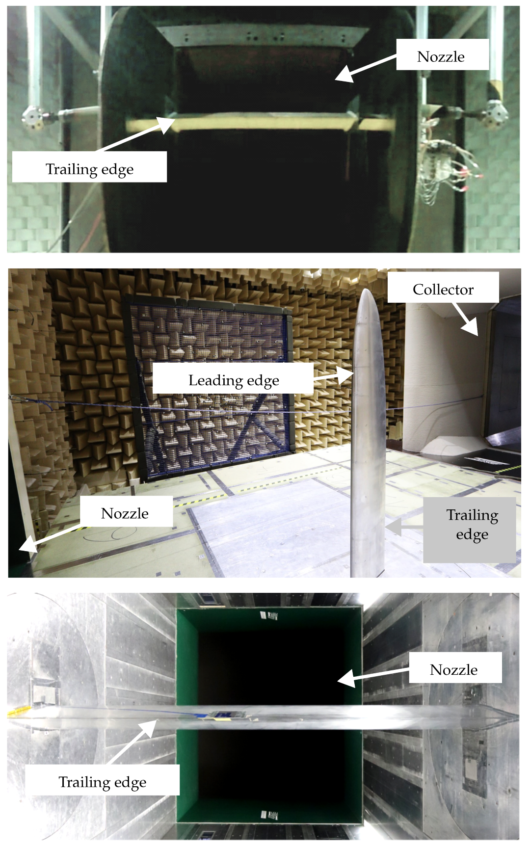Figure 1 illustrates the test setups for each airfoil.

Each of the three wind tunnel models has a different chord length c and span length b.

Table 1. Details on datasets with respect to airfoil type, chord length c, spanwise extension b, Reynolds number ${\mathrm{Re}}_c$, and angle of attack ${\alpha }_{\mathrm{g}}$.

(#1) DU96-W-180 (AWB, Open Test Section)
c (b) [mm]	Config	${\mathrm{Re}}_c$$\times {10}^{-6}$	${\alpha }_{\mathrm{g}}$ [∘]
300 (800)	Tr-0510	0.8; 1.0; 1.2	0; 6; 8; 11; 12; 13; 14; 14.7
(#2) NACA 64-618 (NWB, 3/4-Open Test Section)
c (b) [mm]	Config	${\mathrm{Re}}_c$$\times {10}^{-6}$	${\alpha }_{\mathrm{g}}$ [∘]
344 (2100)	Clean	0.8; 1.0; 1.1; 1.3; 1.5	0; 2; 4; 5; 8; 10; 12; 18; 20; 21; 23
344 (2100)	Tr-0510	0.8; 1.0; 1.1; 1.3; 1.5	0; 2; 4; 6; 9; 10; 13; 16; 18; 20; 21; 23
344 (2100)	Tr-2510	0.8; 1.0; 1.1; 1.3; 1.5	0; 2; 4; 6; 9; 10; 13
(#3) NACA 633018 (NWB, Closed Test Section)
c (b) [mm]	Config	${\mathrm{Re}}_c$$\times {10}^{-6}$	${\alpha }_{\mathrm{g}}$ [∘]
900 (2800)	Clean; Tr-0510; Tr-1010	1.9; 2.8	0; 1; 2; 3; 4; 5; 6; 7; 8; 9; 10; 11; 12; 13; 14; 15; 16; 17
900 (2800)	Clean; Tr-0510; Tr-1010	3.7; 4.5	0; 1; 2; 3; 4; 5; 6; 7; 8; 9; 10; 11; 12; 13; 14; 15; 16

summarizes key details of the wind tunnel models, including airfoil type, chord length c, span length b, and the tripping configuration (config). A clean configuration means that no manipulation was applied and the laminar–turbulent transition occurred naturally. The entry Tr-xxyy indicates that the laminar–turbulent transition was forced using a zig-zag band. Here, Tr denotes tripping, xx the position (in %) of the tripping band on the suction side, and yy the position of the tripping band on the pressure side. Information is also provided on the chord-based Reynolds numbers ${\mathrm{Re}}_c$, which were varied by changing the flow velocity u_∞. Furthermore, an overview of the variation in the AoA within each dataset is given. Note that in this study, AoA always refers to the geometric angle ${\alpha }_{\mathrm{g}}$ set in the wind tunnel.

Each AoA was combined with each Reynolds number ${\mathrm{Re}}_c$ and each tripping configuration, resulting in 384 individual combinations, in which eight flush-mounted sensors captured the surface pressure fluctuations within the given chordwise range. The sensors were implemented in the wind tunnel model, mostly on the suction side, but occasionally also on the pressure side. As flow separation is expected only on the suction side, the measurements on the pressure side are not taken into account.

Table 2. Sensor types utilized within the measurement campaigns ID #1 to #3, the position ranges in the chordwise direction (position spanwise = midspan), and sampling rate. For all three campaigns, 8 sensors were utilized, and the acquisition time was 30 s each campaign.

ID	Sensor Type	Position Range	Sampling
		Chordwise [-]	Rate [Hz]
#1	Kulite LQ-062-0.35BarA	$0.471c–0.957c$	100,000
#2	GRAS 48LX-1	$0.586c–0.834c$	102,400
#3	GRAS 48LX-1	$0.828c–0.923c$	64,000

provides an overview of the sensor types utilized within each measurement campaign, the number of sensors, the position in the chordwise direction, and the sampling rate.

The data from all these measurements were used for the development and evaluation of the flow prediction model. Specifically, the surface pressure fluctuations were used for this purpose for the entire acquisition time measured between $0.5c$ and $1c$. In the low-frequency range, the data below 200 Hz are not reliable due to wind tunnel background noise and potential sensor installation-induced noise [19]. In the upper frequency range, the data is limited to approximately 10,000 Hz due to the attenuating characteristics of the $\raisebox{1ex}{$1$}\!\left/ \!\raisebox{-1ex}{$4$}\right.$-inch-diameter sensor (model GRAS 48LX-1, GRAS Sound & Vibration, Holte, Denmark) and due to the Helmholtz resonant frequency of sensor #1 (model LQ-062-0.35 BarA, Kulite Semiconductor Products, Leonia, NJ, USA) placed under a 0.5 mm diameter pinhole [20].

2.2. Statistics of Surface Pressure Fluctuations

In wall turbulence analysis, a standard practice is to examine the probability density function (PDF) of the pressure fluctuations $p^{\prime }$, which provides insight into the occurrence, intensity, and symmetry of the fluctuations along the chord [21]. To encompass the full dynamics of a separating turbulent boundary layer, a recent study [3] compared a canonical flat plate and two different airfoils, including the DU96-W-180 used in the present study. As argued in [3], non-stochastic high-amplitude events are likely caused by the formation of coherent structures present in separated flows. Typically, changes in the pressure fluctuation PDFs can be analyzed with the skewness $Sk\left(p^{\prime }\right)$ and kurtosis $Ku\left(p^{\prime }\right)$ along the chord, which represent the third and fourth moment of surface pressure fluctuations. On top of the classical spectral information, such time-domain criteria characterize the shape of the PDF of $p^{\prime }$, and certain thresholds of these high-order moments can ultimately be related to a flow map of either attached or separated flow as in [2]. One of the long-term goals in wind energy applications is to monitor the occurrence of flow separation, which can lead to acoustically relevant events. Such detrimental flow conditions therefore require more detailed information about the flow status, ranging from a decelerated but still mean-attached boundary layer to weakly or largely separated states. Le Floc’h et al. [3] indicated that massive flow separation is characterized by a dominant low-frequency contribution in the high-order moments. Unfortunately, such a distinction is presently impossible to achieve considering that the experimental limitations would have required resolution of frequencies lower than 100 $\mathrm{Hz}$ [3,15].

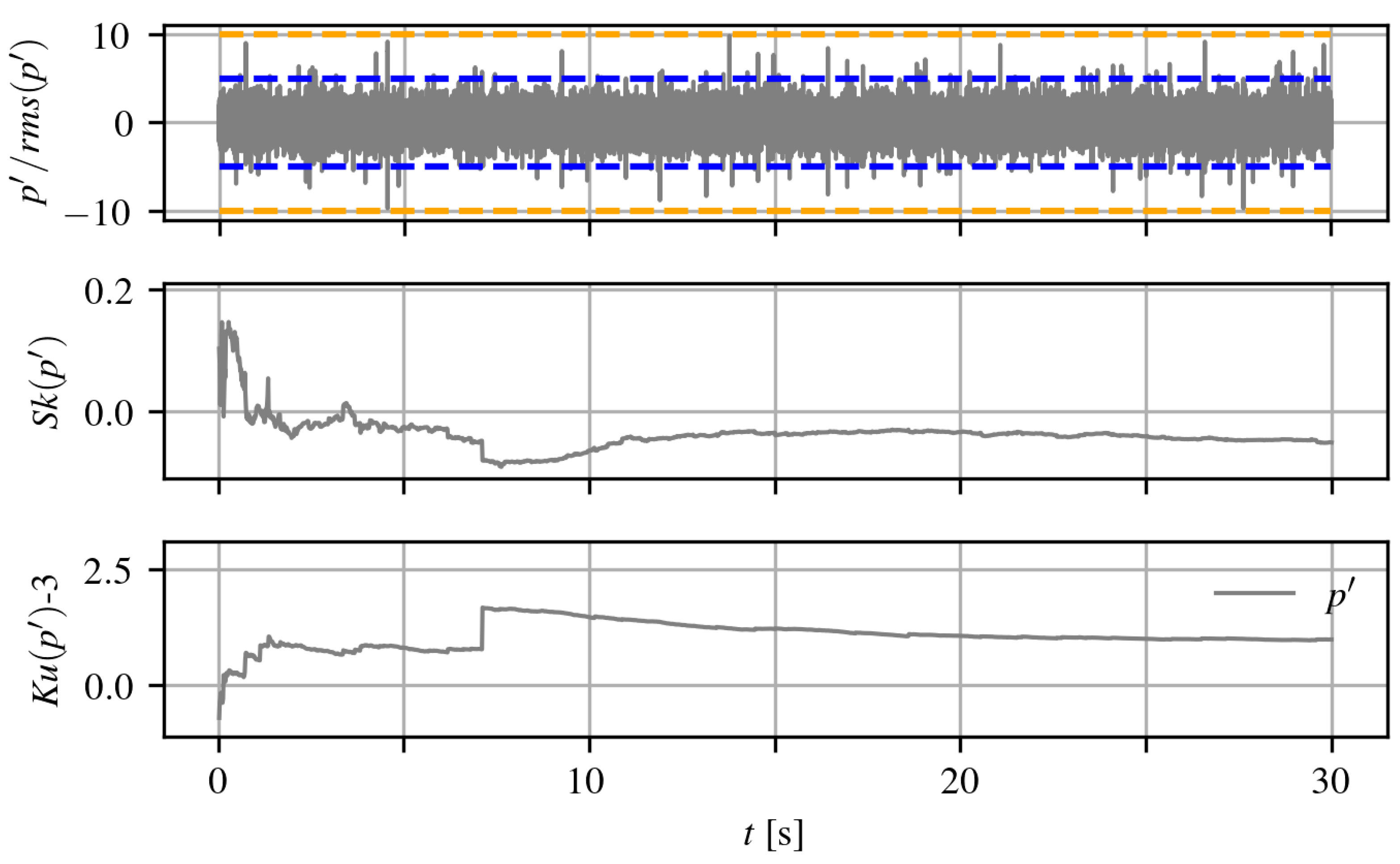
Different types of instrumentation were also used: Kulite sensors for the DU96-W-180 case and GRAS ones for the two NACA profiles. Considering these experimental limitations, the objective is to confirm the global trends observed in [2,3], where the original time traces allowed the definition of thresholds for high-order moments, provided that convergence is achieved. Figure 2 shows the normalized time trace $p^{\prime }/\mathrm{rms}\left(p^{\prime }\right)$, where $\mathrm{rms}\left(p^{\prime }\right)$ denotes the root mean square of the pressure fluctuations, as well as the skewness $Sk\left(p^{\prime }\right)$ and kurtosis $Ku\left(p^{\prime }\right)$ for a case in which flow separation is present. This was measured for dataset #1 DU96-W-180 at ${\mathrm{Re}}_c=1.2\times {10}^6$ and ${\alpha }_{\mathrm{g}}=14.7°$ by a Kulite sensor located at $x/c=0.81$. The peaks typically observed range within $\pm 10\mathrm{rms}\left(p^{\prime }\right)$, which allows the cumulative skewness and kurtosis values to converge to an asymptotic value within a relatively narrow margin of about $\pm 0.05$ and $\pm 0.1$, respectively. The high-order moments also consistently converge after approximately half the length of the time trace, i.e., after about 15 $\mathrm{s}$.

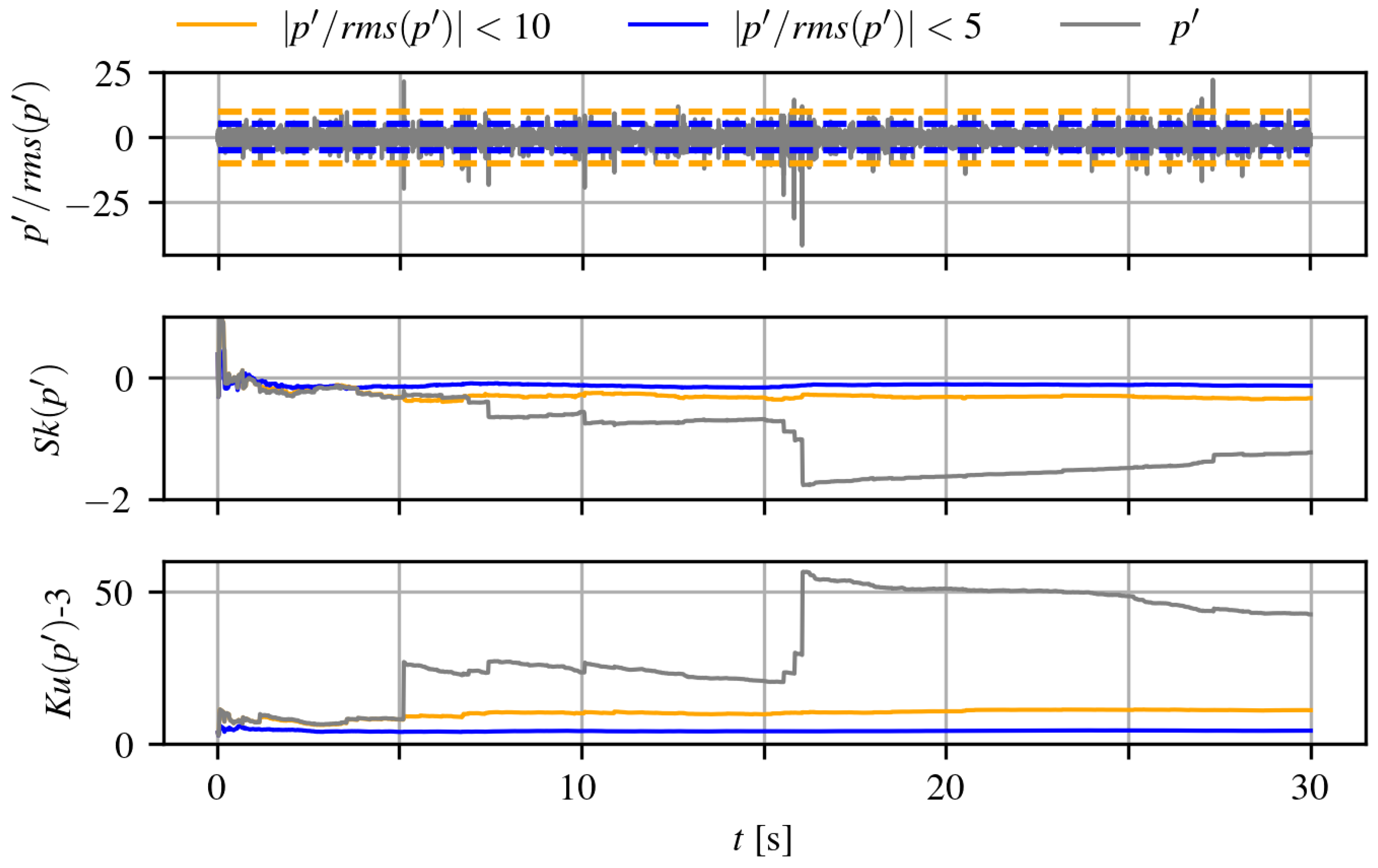
When analyzing dataset #3 with the NACA ${63}_{3}018$ airfoil, GRAS sensors recorded a comprehensive range of angles of attack and multiple inlet reference velocities. A typical result of these sensors at high AoA is shown in Figure 3, where some visible differences can be noted when comparing it to Figure 2, as the separated-flow conditions for the NACA ${63}_{3}018$ are observed at ${\mathrm{Re}}_c=1.9\times {10}^6$. Unlike the results from the Kulite sensors, note the different scales of the y-axes. Indeed, Figure 2 exhibits numerous instantaneous points with abnormally high-amplitude pressure peaks, which can be defined as $\left|p^{\prime }\right|>10\mathrm{rms}\left(p^{\prime }\right)$.

To the best of the authors’ knowledge, such high values are not associated with coherent structures in the literature on separated flows and they are likely not connected to any physical motion. However, the immediate effect of such abnormal extreme values results in the poor convergence of both the cumulative skewness and kurtosis. When the events with $|p^{\prime }| >5 \mathrm{rms}\left(p^{\prime }\right)$ and $|p^{\prime }| >10 \mathrm{rms}\left(p^{\prime }\right)$ are excluded, a satisfactory convergence is obtained, and the upper threshold of 10 $\mathrm{rms}\left(p^{\prime }\right)$ appears sufficient. Therefore, trimming these very-high-amplitude pressure peaks provides an adequate solution for amplitude correction and enables a better interpretation of results in the time domain.

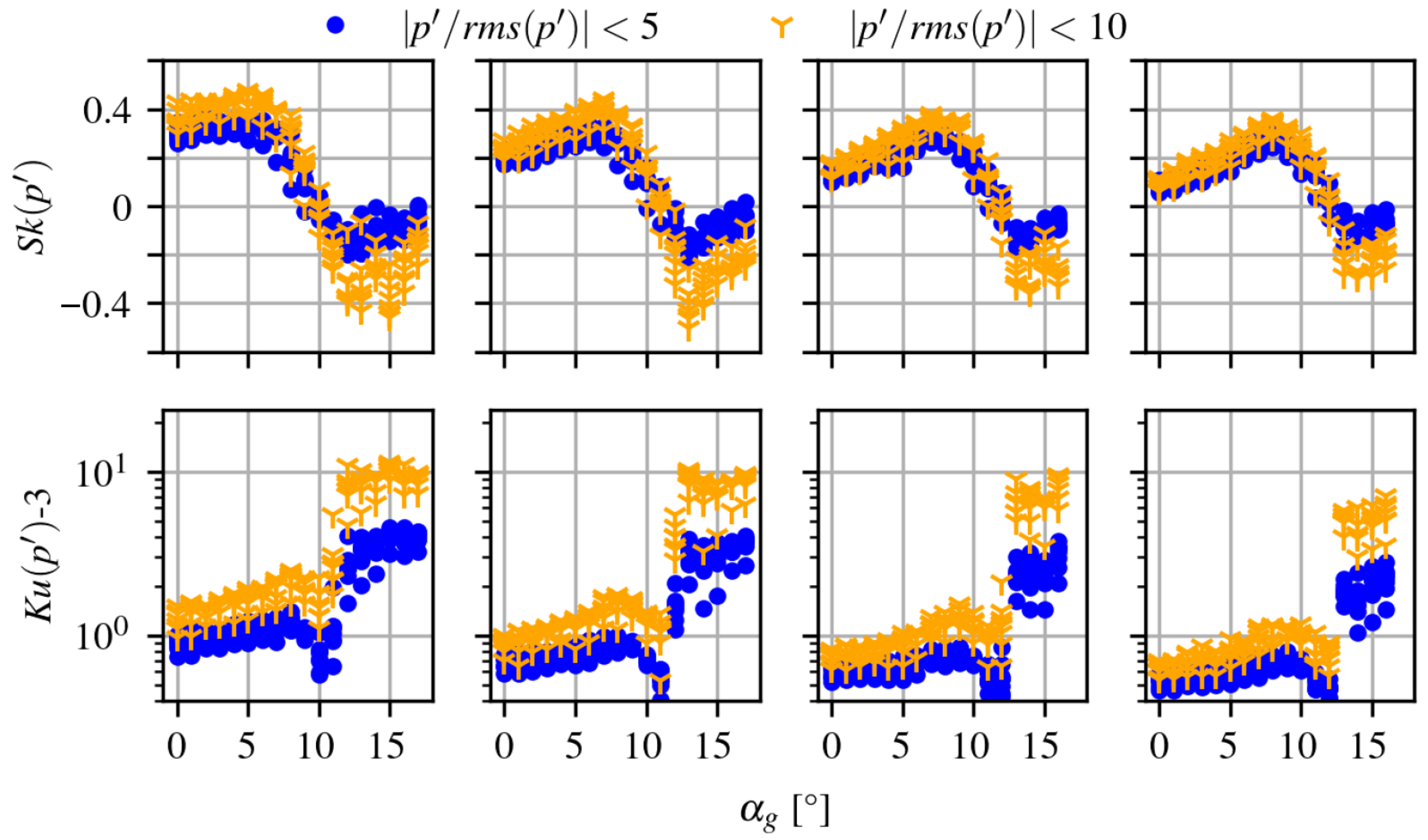
Figure 4 presents the skewness and kurtosis of the two different corrections of the time signals, where the very-high-amplitude pressure peaks were excluded using two thresholds, $|p^{\prime }| >5 \mathrm{rms}\left(p^{\prime }\right)$ and $|p^{\prime }| >10 \mathrm{rms}\left(p^{\prime }\right)$. The wide array of measurements for the AoA allow the range ${\alpha }_{\mathrm{g}}=0°–17°$ for the two Reynolds numbers ${\mathrm{Re}}_c=1.9\times {10}^6$ and $2.8\times {10}^6$ to be covered, as well as the range ${\alpha }_{\mathrm{g}}=0°–16°$ for ${\mathrm{Re}}_c=3.7\mathrm{and}4.5\times {10}^6$. The trends are remarkably consistent with the global observations of Le Floc’h et al. [3], where the onset of separation was characterized by positively skewed wall pressure.

In the present study, the full streamwise extent of the chord is not covered. Within each combination of measurements, eight sensors located in the last 25% of the chord simultaneously measured the surface pressure fluctuations from which skewness and kurtosis were calculated. It is worth noting here that the skewness and kurtosis values are remarkable for separated cases. With increasing AoA, a natural equivalence between a streamwise evolution toward the middle of a recirculation region and increasing values of ${\alpha }_{\mathrm{g}}$ can be made in order to appreciate the effects of a progressively stronger flow separation. Beyond ${\alpha }_{\mathrm{g}}>10°$, a switch from positive to negative skewness is observed for all cases. Consistently with [3], the more negatively skewed values are obtained for the lowest velocities as they correspond to larger separation cases at ${\mathrm{Re}}_c=1.9\times {10}^6$ than at ${\mathrm{Re}}_c=4.5\times {10}^6$. Regarding the kurtosis distribution, a first local peak is obtained for ${\alpha }_{\mathrm{g}}=7°–8°$, where the skewness reaches its positive maximum at the onset of separation. A second kurtosis peak occurs when the sign of the corresponding skewness abruptly switches from positive to negative as the vortex shedding unsteadiness is triggered in the recirculation region. With proximity to the trailing edge, skewness values decrease while kurtosis values increase. These features were also observed for the flat plate under massive flow separation, whereas no sign change in skewness was observed for an adverse-pressure-gradient turbulent boundary layer, still attached in a mean sense.

However, to obtain converged higher-order moments, a long time trace is necessary, which prohibits any separation detection in the case of real-time application. This limitation motivates a shift toward spectral features, which reduce the data volume and can be extracted on short time scales, potentially within a second, thus offering a more practical foundation for real-time prediction of separation. Beyond this immediate benefit, the use of spectral inputs also facilitates systematic comparisons across datasets and geometries, thereby strengthening both the robustness and the generalizability of machine-learning-based detection approaches.

3. Machine Learning Framework

Machine learning (ML) techniques can generally be divided into supervised and unsupervised methods. Supervised ML uses algorithms to create models that predict future values based on input data, requiring labeled datasets, while unsupervised methods operate without labels. In this study, the prediction of the flow status, whether attached or separated, constitutes a supervised binary classification problem.

Different techniques are available to solve such a classification problem. The ML techniques multilayer perceptron (MLP), support vector machine (SVM), and logistic regression (LR) were evaluated for this purpose. A brief description of these will be given in Section 3.1. For a more detailed overview, the reader is referred to [22]. Section 3.2 details data preprocessing including labeling and preparation for ML. The performance of the various algorithms is evaluated based on accuracy (ACC), the Matthews correlation coefficient (MCC), sensitivity (Se), and specificity (Sp). These metrics are briefly explained in Section 3.3.

3.1. Applied Machine Learning Methods

In the following, the three selected ML methods are briefly introduced to outline their underlying principles and the specific configurations used in this study.

3.1.1. Multilayer Perceptron

MLP [23] is a simple and frequently used type of neural network that generalizes the classical perceptron to handle data that is not linearly separable. This is achieved by organizing perceptrons in successive layers, such that the outputs of all perceptrons in one layer serve as the weighted input to all perceptrons in the next layer. Non-linear behavior arises when activation functions (e.g., rectified linear unit (ReLU) or Sigmoid) are introduced between the layers. Optimal weights can be found by minimizing a loss function using, e.g., the standard backpropagation algorithm, depending on a small number of hyperparameters such as the learning rate or batch size.

Various model sizes, activation functions, and hyperparameters were studied and implemented in PyTorch [24] based on a training scheme that batches the training data and adjusts the learning rate following an exponential decay schedule; also see

Table 3. Varied hyperparameters for MLP with $N_{\mathrm{layers}}\in \{2,3,4,6,8\}$ (the number of neurons in the first layer was 785 and decreased equidistantly from layer to layer) and activation functions ReLU and Sigmoid.

Initial Learning Rate	Learning Rate Decay	Batch Size
0.010; 0.011; …; 0.019	0.9998	32
0.02; 0.025; 0.03
0.015	0.9998	16; 64; 128
0.015	0.999; 0.9995	32

. The loss function to be minimized by the training routines is the standard binary cross-entropy. In addition, we tested whether post-training quantization of the fully trained MLPs, i.e., lowering the numerical precision to speed up computations, reducing the memory footprint, and improving energy efficiency, is advantageous [25]. Among many implementations tested, PyTorch’s post-training dynamic quantization from 32-bit floating point (FP32) to 8-bit integer (INT8) stood out with a minimal degradation in prediction performance but significant speed-ups and only one quarter of the memory footprint.

The quantization is “dynamic” in the sense that all model weights are converted to INT8 once after training, but activation functions are dynamically quantized “on the fly” during each forward pass.

3.1.2. Logistic Regression

LR is a classification algorithm that estimates class probabilities using the logistic function applied to a linear combination of input features. LR determines the decision boundary based on these probabilities. With larger datasets, the model’s classifications become more accurate, yet some degree of uncertainty and potential for misclassification remain. To optimize LR performance, several hyperparameters were varied, including the regularization parameter C, the solver used, and the maximum number of iterations allowed, $N_{\mathrm{maxit}}$. The regularization techniques (penalties) were applied as follows: L2 regularization and no penalty were tested with the lbfgs, newton-cg, newton-cholesky, sag, and saga solvers; L1 and L2 regularization were tested for the liblinear solver; and elasticnet, L1, L2, and no penalty were evaluated for the saga solver.

Table 4. Hyperparameters tested for logistic regression, including solvers, regularization parameters C, and maximum number of iterations $N_{\mathrm{maxit}}$.

Parameter	Values
Solver	lbfgs; liblinear; newton-cg; sag; saga; newton-cholesky
C	0.001; 0.01; 1
$N_{\mathrm{maxit}}$	100; 1000; 2500; 5000; 10,000

provides an overview of the varied hyperparameters for the investigated solvers.

3.1.3. Support Vector Machine

SVM models are closely related to classical MLP neural networks and are based on the concept of maximizing the margin between the separating hyperplane and the data points. This margin maximization aims to reduce the expected generalization error [26].

SVMs have several hyperparameters that can be tuned to improve performance, including the kernel type, penalty weight (C), and kernel function parameter gamma. The kernel type determines the functional form of the separating hyperplane, while C and $\Gamma$ control its complexity. In this study, the hyperparameters of the SVM models listed in

Table 5. Hyperparameters tested for support vector machine (SVM).

Parameter	Values
Kernel types	linear, rbf, polynomial, sigmoid
$\Gamma$	1; 0.1; 10; 100; 1000
C	0.1; 1; 10; 100; 1000

were systematically explored.

Grid search was implemented using the Scikit-learn library to identify the optimal hyperparameter settings for the present task when using SVMs [27].

3.2. Data Preprocessing

This section describes the preprocessing of the experimental data. It first explains the labeling procedure used to assign flow states (Section 3.2.1) and then outlines the preparation steps applied to normalize, clean, and split the data for machine learning (Section 3.2.2).

3.2.1. Labeling of the Data

To evaluate whether flow separation was present, three key indicators were considered: (i) the power spectral density (PSD) of surface pressure fluctuations, (ii) the static surface pressure distribution, and (iii) the lift coefficient. The lift coefficient is proportional to the AoA over a wide range as long as the flow remains attached. However, once it deviates from the linear range, this indicates the onset of flow separation [28,29]. Another important indicator of flow separation is its relationship with the static surface pressure distribution. When the flow separation occurs, it is often observed that the pressure distribution on the suction side forms a plateau extending from the onset of separation to the trailing edge [28,29].

Adverse pressure gradients slow down the flow, with a stronger effect close to the wall, ultimately inducing flow separation. In this study, the adverse pressure gradient was modified by changing the angle of attack. In the PSD of the surface pressure fluctuations, flow separation can be recognized by a shift in the maximum peak to lower frequencies accompanied by a significant level increase of about 10 dB [30]. If the flow separation becomes more pronounced, the spectral decay becomes more rapid and starts earlier [15]. Two different slopes, adopting the shape of an elbow, can often be recognized within the mid-frequency range [31].

To demonstrate how the pressure distribution $C_p$ and the PSD of the surface pressure fluctuations reflect the onset, incipient, and fully developed flow separation, corresponding figures have been prepared. Specifically, dataset #3 (NACA 64-618, at $u_{\infty }=70 \mathrm{m}/\mathrm{s}$, Tr-0510) was chosen. Three angles of attack ${\alpha }_{\mathrm{g}}=6^{°},10°,\mathrm{and}13°$ were selected based on the state of flow separation: attached, incipient, and separated. Figure 5 depicts the pressure distribution.

For ${\alpha }_{\mathrm{g}}=6°$, no plateau can be seen on the suction side. In addition, the pressure coefficient decreases on the suction side in the last quarter of the chord. For ${\alpha }_{\mathrm{g}}=10°$, a small plateau appears on the suction side, denoting the beginning of a flow separation. For ${\alpha }_{\mathrm{g}}=13°$, a pronounced plateau forms in the pressure distribution, indicating a separated flow.

The PSD of the surface pressure fluctuations is presented in Figure 6. As the AoA increases, the peak shifts clearly toward lower frequencies. The rise in the level can also be observed for ${\alpha }_{\mathrm{g}}=10°$ and ${\alpha }_{\mathrm{g}}=13°$. For ${\alpha }_{\mathrm{g}}=13°$, the presence of flow separation is characterized by two elbow-shaped slopes.

Hence, the lift coefficient $C_l$, the static pressure distribution $C_p$, and the PSD of the surface pressure fluctuations were utilized to classify the data with respect to the presence of flow separation and labeled accordingly. Finally, Figure 7 summarizes the mean spectra in ${\mathrm{Pa}}^2/\mathrm{Hz}$ and their standard deviation across all datasets for each flow state, i.e., separated or attached.

Although overlaps exist between the mean and standard deviation for an attached and separated flow, the increase in the level in the low-frequency range and the decrease in the spectrum for the separated flow are illustrated once again. The mean of the attached samples initially remains constant over a large frequency range.

3.2.2. Data Preparation

Data preparation is a crucial step in ML analysis. Thereby, planning ahead to rationalize and improve data preparation can lead to more accurate and adaptable ML algorithms. In the herein-proposed approach, it mainly consists of four steps, which were implemented as described below.

First, non-physical samples, presumably due to a malfunction of the sensor, were excluded from the entire dataset. Second, the samples were interpolated to identical lengths to ensure consistent frequency resolution of $12.5$ $\mathrm{Hz}$ for the selected frequency range of 200 to 10,000 Hz. Third, the data were normalized so that the absolute values were constrained to be ≤1. Subsequently, the considered data were split into three sets for different purposes: training set, validation set, and test set. The training set accounted for 70% of the data, while the validation and test sets each comprised 15%. The test and validation sets are independent of the training data, but should have the same distribution of features as the training dataset. The validation set was used for hyperparameter selection of the respective ML models. The test set was used for the evaluation of the final selected ML model. The split of the data was generated automatically with a fixed seed in order to proceed deterministically when training the various ML models. Care was taken to ensure that the distribution across the respective datasets was balanced, particularly with respect to the following features: airfoil geometry, AoA, flow velocity, and flow status. The resulting distribution for the training, validation, and test sets along the features mentioned is illustrated in Figure 8.

3.3. Evaluation Metrics

Initially, hyperparameter optimization was performed for each applied ML method using validation data, to select the best configuration for each technique. The optimal model was then selected based on two evaluation metrics: accuracy and Matthews correlation coefficient. The accuracy (ACC), which is also called observed agreement, is defined as

$$ACC={\displaystyle \frac{\mathrm{TP}+\mathrm{TN}}{\mathrm{TP}+\mathrm{FP}+\mathrm{TN}+\mathrm{FN}}}$$

(1)

with TP denoting the number of true positives, FP the false positives, TN the true negatives, and FN the false negatives among the predicted cases. It represents the proportion of correct classifications among all predictions. Sensitivity and specificity were also considered to provide a more comprehensive assessment of model performance. Specificity itself can be described as the model’s ability to predict a true negative for each category available. It is also known as the true negative rate and defined as

$$Sp={\displaystyle \frac{\mathrm{TN}}{\mathrm{TN}+\mathrm{FP}}}$$

(2)

For instance, in this study, this can be interpreted as the ability of the model to predict the status of an attached flow for any AoA. Sensitivity in ML can be described as the metric used for evaluating a model’s ability to predict the true positives of each available category. It is also known as the true positive rate and calculated as follows:

$$Se={\displaystyle \frac{\mathrm{TP}}{\mathrm{TP}+\mathrm{FN}}}$$

(3)

In this study, for example, this can be understood as the ability of the model to predict the status of a separated flow for any AoA.

The Matthews correlation coefficient (MCC) is also utilized as an alternative measure of accuracy [13]. It is particularly advantageous compared to other measures of agreement, such as Cohen’s kappa, as it effectively handles imbalanced class distributions. This is crucial in our case, since the occurrence of flow separation is not evenly represented across the considered features. The MCC evaluates the quality of binary classifications based on a contingency matrix, taking into account true and false positives as well as true and false negatives, and thus providing a more balanced assessment even in cases of class imbalance. It can be formulated as

$$MCC={\displaystyle \frac{\mathrm{TP}·\mathrm{TN}-\mathrm{FP}·\mathrm{FN}}{\sqrt{(\mathrm{TP}+\mathrm{FP})(\mathrm{TP}+\mathrm{FN})(\mathrm{TN}+\mathrm{FP})(\mathrm{TN}+\mathrm{FN})}}}$$

(4)

4. Results and Discussion

In this section, we present and analyze the outcome of applying the different ML techniques from Section 3 based on data from the test and validation sets, i.e., data that was not used during training. For this purpose, quantities such as model size, (wall clock) training and forward-pass time, and the Matthews correlation coefficient (MCC) are considered, and the most suitable ML model is selected.

4.1. Results: Multilayer Perceptron

All MLPs were trained serially on two Intel^® Xeon^® Gold 6230 CPU @ 2.10 GHz (20 cores, 40 threads; Intel Corporation, Santa Clara, CA, USA) and optimal hyperparameters were determined based on the performance on the validation dataset. In terms of both training stability and the MCC of the final MLPs, the ReLU activation functions clearly outperformed the Sigmoid functions in all scenarios. Regarding number of layers, networks with two layers showed the lowest MCC and accuracy values. Models with three or four layers achieved similar results in MCC and accuracy. For six and eight layers, the training accuracy often reached a value of 1.0 while the accuracy and the MCC value did not improve compared to fewer layers, indicating overfitting for these model sizes. For the activation function Sigmoid, models with a number of layers of six and eight did not converge and therefore were not considered further. In total, the most promising MLP in FP32 precision that was tested consisted of three linear layers and ReLU activation functions in between, and it was best trained with an initial learning rate of 0.017, decreasing with an exponential decay rate of 0.9998. The model achieved a prediction accuracy of 0.977 and an MCC of 0.989 on the test set. This model trained on the above hardware for approximately $1.6$ $\mathrm{s}$ and required about 7 $\mathrm{m}$$\mathrm{s}$ to classify a single input pattern. The model required a memory of 2.6 MB. Post-training dynamic quantization from FP32 to INT8 reduced the memory footprint to 0.7 MB, i.e., shrinking by the expected factor of four, while the time for a single forward pass was reduced to 4.333 ms. However, these advantages come at the price of small penalties in accuracy (−0.005) on the test set and in the MCC (−0.010).

4.2. Results: Logistic Regression

The LR runs were executed serially on a system with an Intel^® Core^™ i7-8665U CPU @ 1.90 GHz (four cores, eight threads). The hyperparameter studies for LR, presented in Section 3.1.2 in Table 4, showed that the choice of the solver newton-cg performed best in combination with the penalty L2, a C value of 100, and a maximum number of iterations of 100. Training time of the model on the training set was $0.67$ $\mathrm{s}$, and a prediction (forward-pass time) for a single sample took $0.003$ $\mathrm{m}$$\mathrm{s}$. The model required only 7 kB of memory. On the test set, the model achieved a prediction accuracy of 0.964 and an MCC of 0.927.

4.3. Results: Support Vector Machine

The runs for SVM were executed serially on a system with an Intel^® Core^™ i7-8665U CPU @ 1.90 GHz (four cores, eight threads). For the hyperparameters varied for SVM—see Section 3.1.3—the kernel rbf performed best in combination with a gamma value of 1 and a C value of 100. The model achieved a prediction accuracy and MCC of 0.990 and 0.980 on the test set. The training time of the model on the training set was $0.83$ $\mathrm{s}$, and a prediction (forward-pass time) based on a single sample without preprocessing took $0.18$ $\mathrm{m}$$\mathrm{s}$. The model required a memory of 1.4 MB.

A compact summary of the results of the pre-selected ML models is presented in

Table 6. Comparison of model size, training time (on training set), forward-pass time (on one sample), Matthews correlation coefficient (MCC), and accuracy for ML techniques (MLP, Q-MLP, LR, and SVM) with optimized hyperparameters.

	MLP	Q-MLP	LR	SVM
Model size [kB]	2611	660	7	1380
Training time [s]	1557	-	0.67	0.83
Forward-pass time [ms]	7.301	4.333	0.003	0.179
MCC	0.977	0.967	0.927	0.980
Accuracy	0.989	0.984	0.964	0.990

. Here, the SVM model performed best, with an MCC of 0.980 and an accuracy of 0.990. Another important criterion, especially regarding the model’s intended real-time capability, is the forward-pass time. For this parameter, the LR model achieved the best results with 0.003 ms, followed by the SVM model with 0.179 ms. In terms of storage capacity, the LR model required the least memory with just 7 kB, followed by the quantized MLP model with 0.7 MB and the SVM model with 1.4 MB. With 2.6 MB, the MLP model requires twice as much memory as the SVM model.

4.4. Assessment of ML Results

The SVM model was selected as the most suitable for detecting flow separation due to its by prediction accuracy and speed. The superior performance of both the SVM and MLP models compared to LR can likely be attributed to their ability to capture non-linearities in the transition from attached to separated flow. LR, being inherently linear, struggles with this complexity, leading to its lower prediction accuracy. In terms of accuracy, SVM, MLP, and Q-MLP performed on a similar level (Table 6), with SVM performing slightly better than the others. This overall slight edge of SVM might be attributed to its strategy of projecting data into a higher-dimensional space, enabling it to more effectively capture non-linear boundaries between flow states.

Regarding the prediction speed, SVM clearly outperformed MLP and Q-MLP by a factor of about 40 compared to MLP and 24 compared to Q-MLP. To ensure a fair comparison, the models were all run on the same hardware as that used to train SVM and LR. Following the identification of potential reasons for the superior performance of the SVM model, the test set data were analyzed in more detail to evaluate the practical accuracy of the predictions. Since separation becomes more likely with a higher AoA, and thus the AoA is an important parameter, different metrics as a function of the AoA were considered for the selected model. These include the confusion matrix, sensitivity, and specificity. Figure 9 depicts the confusion matrix, which consists of four key metrics: TP, FP, TN, and FN.

The TN and TP can be associated with groups of low and high angles of attack, respectively. Low angles of attack correspond to the TN field, while higher angles of attack correspond to the TP field. This result was expected, since flow separation is unlikely at low angles of attack and becomes more likely as the angle increases. In addition, there is a transition region where the model correctly predicts the status of the flow for both cases (attached and separated) for the same AoA. Flow separation depends on airfoil geometry and Reynolds number. Therefore, the AoA at which flow separation begins varies. Furthermore, the flow separation begins in the vicinity of the trailing edge and shifts further upstream as the AoA increases. Now consider two sensors under identical flow conditions and incipient flow separation, where one is placed in the vicinity of the trailing edge and the other further upstream. The signature of the flow separation will be present at the sensor in the vicinity of the trailing edge, but not at the one further upstream. The ML model makes accurate predictions here. However, it should be mentioned at this point that the captured signal can consist of both flow states, especially in the medium-AoA range, as the separation point can vary locally. This may explain the cases in the FP and FN fields, as the model produced incorrect predictions for a few measurements. At the same time, however, possible inaccuracies in data labeling must also be considered.

Figure 10 summarizes the results from the confusion matrix and presents them in relative metrics using sensitivity, specificity, and accuracy over AoA. As no flow separation was observed for AoAs below 7°, no meaningful results for sensitivity are available in this range. Conversely, for AoAs of 16° and above, only cases with flow separation were observed, so no meaningful results are available for specificity for higher AoAs.

Figure 10 demonstrates that the model has a high prediction capability at both low and high AoAs. With $Sp=1$ for the AoA range ${\alpha }_{\mathrm{g}}=0°–10°$, the specificity reveals that the model predicts the status of an attached flow with nearly no errors. For ${\alpha }_{\mathrm{g}}>10°$ the specificity decreases progressively.

As mentioned above, this may result from a mixture of flow states within a single measurement or from inaccuracies in data labeling. It was also observed that the samples where the sensors were placed further upstream were predicted incorrectly relatively often. In addition, only a few samples exist in the peripheral regions, which means that outliers become more significant. For the same reasons, the sensitivity also starts with lower values of $Se=0.88$ at ${\alpha }_{\mathrm{g}}=8°$, but increases rapidly with AoA and remains close to Se = 1 except for ${\alpha }_{\mathrm{g}}=20°$, where a single outlier reduces it to $Se=0.90$.

5. Conclusions and Outlook

A binary method for the detection of flow separation has been presented, where three different ML algorithms were trained, their hyperparameters were optimized and tested, and a final ML model was selected. The power spectral density of experimentally measured surface pressure fluctuations was used as input. The SVM model has proven to be the most suitable for binary classification compared to MLP and LR in terms of prediction accuracy, the MCC, and execution time. The accuracy of the SVM model determined with the test dataset was 0.985, and the MCC was 0.975. An advantage of the presented method is the flexibility of the pressure sensor placement within the last 30% of the chord. Regardless of the sensor positions in this area, the model was able to predict the status of the flow separation reliably. This allows flexibility in sensor placement in real applications where the detection of flow separation is required. Only at the transition to flow separation, i.e., at medium angles of attack, is the sensitivity of the model at a moderate value of $Se=0.880$ and the specificity at an acceptable $Sp=0.860$.

Two main paths are now proposed for future research. First, the development of a multiclass prediction model is planned, which would classify the flow separation into several severity levels. This advancement could provide more detailed insights into flow dynamics and support more targeted mitigation measures based on the acoustic relevance of the flow separation. Second, future studies will determine how short the time signals can be made while still maintaining reliable model predictions. Once this limit is established, the method’s real-time performance will be tested in a dedicated wind tunnel campaign on a truncated wind turbine blade tip, representing a decisive step toward transferring the approach from controlled wind tunnel profiles to a realistic application.